Stringy Signals from Large-Angle Correlations in the Cosmic Microwave Background?

Abstract

We interpret the lack of large-angle temperature correlations and the even-odd parity imbalance observed in the cosmic microwave background (CMB) by COBE, WMAP and Planck satellite missions as a possible stringy signal ultimately stemming from a composite inflaton field (e.g., a fermionic condensate). Based on causality arguments and a Fourier analysis of the angular two-point correlation function, two infrared cutoffs $k_{\min }^{\mathrm{even},\mathrm{odd}}$ (satisfying $k_{\min }^{\mathrm{even}}\simeq 2k_{\min }^{\mathrm{odd}}$) are introduced to the CMB power spectrum associated, respectively, with periodic and antiperiodic boundary conditions of the fermionic constituents (echoing the Neveu–Schwarz–Ramond model in superstring theory), without resorting to any particular model.

1. Introduction

Since its discovery in 1964 by Penzias and Wilson, the study of the cosmic microwave background (CMB) has provided a wealth of information on the early universe and its evolution, even going back in time closer to the Big Bang than the recombination phase when it was released. Indeed, to account for the outstanding homogeneity of the CMB temperature across the sky, an inflationary phase has been put forward to solve the so-called horizon problem, together with the flatness issue and “unwanted” relics, such as unseen magnetic monopoles [1].

Although there are alternative models, inflation has currently become the commonly accepted paradigm to explain cosmological evolution because of a series of convincing reasons, of which we just highlight one: observations of the CMB temperatures across the sky show that the universe is approximately uniform and homogeneous at scales much larger than the particle horizon at decoupling time, and a phase of exponential growth can account for this.

In principle, the basic requirement needed for a successful inflation is a scalar field satisfying the slow-roll conditions and a graceful exit. Actually, the inflaton needs not be a fundamental (nor single) scalar field but an effective, e.g., composite, field (see ref. [2] for a review) stemming from more fundamental interacting fields (such as a fermionic condensate1). Through the process of inflation, initial small quantum fluctuations of the underlying inflationary field when exiting the Hubble horizon would have formed the seeds for the matter distribution and subsequent growth to structures seen in today’s universe [5], showing an overall isotropy and homogeneity at large scales. Alternatively, in a linearly expanding cosmology, like the so-called $R_h=ct$ universe (for an exhaustive review of this model, see [6]), the quantum fluctuations of the primordial field driving the expansion turned into (semi-)classical fluctuations once exiting the Planck domain at about the Planck time [7].

On the other hand, in spite of the many successes of the Standard Cosmological Model ($\Lambda$CDM), anomalies and tensions have emerged from a variety of astrophysical and cosmological observations (see, e.g., [8,9,10,11,12,13,14]). In particular, the unexpected lack of large-angle angular correlations (usually related to missing power at low multipoles) observed by all three major satellite missions, COBE [15], WMAP [16] and Planck [17,18], together with the odd-parity preference in the two-point correlation function of the CMB [19,20,21], were examined in detail in Ref. [22]. To this end, an infrared cutoff was set in the primordial CMB power spectrum following the original work of [23]. At the same time, odd-parity dominance was taken into account by weighting the different multipole contributions to angular correlations. Needless to say, such a parity imbalance questions the large-scale isotropy of the observable universe and hence the cosmological principle.

Here we shall perform a similar analysis but while introducing two infrared cutoffs (rather than one) to the CMB power spectrum ($k_{\min }^{\mathrm{even},\mathrm{odd}}$), affecting differently the even- and odd-parity multipole contributions in the best fit of the temperature two-point correlation function $C\left(\theta \right)$ to Planck 2018 data. Firstly, the aim of using two infrared cutoffs, rather than one, is to simultaneously achieve both goals (reproducing missing large-angle correlations and odd-parity dominance) with fewer fitting parameters, while suggesting an interesting and novel physical interpretation. Indeed, large-angle correlations should provide details on the very first stages of the universe, maybe hinting new physics at unexplored large scales, as addressed elsewhere [24,25]. This possibility stands as the main motivation of this paper.

In order to obtain the best fit of $C\left(\theta \right)$ to Planck data, we find that the ratio $k_{\min }^{\mathrm{even}}/k_{\min }^{\mathrm{odd}}$ must be numerically close to two. Later, we will provide a tentative theoretical explanation for this, based on an assumed “stringy”2 behaviour of the fundamental primordial field(s) driving inflation in the early universe.

2. Angular Correlations in the CMB

All three COBE, WMAP and Planck satellite missions have observed that the temperature angular distribution of the CMB is remarkably homogeneous across the sky, with anisotropies of order 1 part in ${10}^5$. A powerful test of these fluctuations relies on the two-point (and higher [28,29]) angular correlation function $C\left(\theta \right)$, defined as the ensemble product of the temperature differences with respect to the average temperature $T_0$ from all pairs of directions in the sky defined by unitary vectors ${\overrightarrow{n}}_1$ and ${\overrightarrow{n}}_2$:

$$C\left(\theta \right)=\langle \frac{\delta T\left({\overrightarrow{n}}_1\right)}{T_0}\frac{\delta T\left({\overrightarrow{n}}_2\right)}{T_0}\rangle ,$$

(1)

where $\theta \in [0,\pi ]$ is the angle defined by the scalar product ${\overrightarrow{n}}_1·{\overrightarrow{n}}_2$.

Assuming azimuthal symmetry, $C\left(\theta \right)$ can be expanded using the Legendre polynomials as:

$$C\left(\theta \right)=\frac{1}{4\pi }\sum _{\ell =2}^{\infty }(2\ell +1)C_{\ell }{P}_{\ell }(cos\theta ),$$

(2)

where the $C_{\ell }$ multipole coefficients encode the information with astrophysical/cosmological significance. In practice, the sum starts at $\ell =2$ and ends at a given ${\ell }_{\max }$, dictated by the resolution of the data (in our case we set $\ell =400$ as an upper limit). The first two terms are excluded because (i) the monopole ($\ell =0$) is simply the average temperature over the whole sky and plays no role in the correlations, other than a global scale shift; and (ii) the dipole ($\ell =1$) is greatly affected by Earth’s motion, creating an anisotropy dominating over the intrinsic cosmological dipole signal, being usually removed from the multipole analysis.

Under some simplifying assumptions [5], the coefficients $C_{\ell }$ in Equation (2) can be evaluated according to the following expression:

$$C_{\ell }=N{\int }_0^{\infty }dk{k}^{n_s-2}{j}_{\ell }^2\left(k{r}_d\right),$$

(3)

where N is a normalization constant, $n_s\approx 1$ is the spectral index and $j_{\ell }\left(k{r}_d\right)$ denotes the spherical Bessel function of order ℓ, whose argument involves the comoving distance $r_d$ from the last scattering surface (LSS) to us, and the wavenumber k for each mode in the CMB power spectrum which varies, in principle, from zero to infinity.

3. Single Infrared Cutoff in the CMB Power Spectrum

As already commented, large-angle temperature correlations in the CMB provide information on the earliest stages of the primitive universe, well before recombination and the subsequent formation of the cosmic structure [5]. In this regard, the $C\left(\theta \right)$ function defined in Equation (2) was found to be close to zero above 60${}^{\circ }$–70${}^{\circ }$ from all three COBE, WMAP and Planck data, constituting one of the anomalies between standard cosmology and observations [8]. Indeed, the suppression of large-angle correlations together with the existence of a downward tail at large angles (≳150${}^{\circ }$) were unexpected in standard cosmology, given that inflation is supposed to provide the required number of e-folds (≥60) to solve both the horizon and flatness problems, thereby bringing angular coverage across the full sky.

In order to mitigate this tension, the authors of [23] introduced an infrared cutoff in the CMB power spectrum, leading to a lower limit $k_{\min }$ in the integral of Equation (3)

$$C_{\ell }=N{\int }_{k_{\min }}^{\infty }dk{k}^{n_s-2}{j}_{\ell }^2\left(k{r}_d\right),$$

(4)

yielding a suppression of large-angle correlations. The normalization constant N and $k_{\min }$ are obtained from a global fit to the whole angular correlation function.

A theoretical motivation to this truncation of k modes entering the integral of Equation (4) relies on a maximum correlation length obtained from a causality requirement at decoupling time $t_d$ [23,30]:

$${\lambda }_{\max }=2\pi R_h,$$

(5)

where $R_h$ stands for the Hubble radius at that time. Actually, the Hubble radius $R_h$ is not necessarily a true horizon, but should provide an order of magnitude estimate of the maximum correlation length based on causality. In fact, ${\lambda }_{\max }=\alpha 2\pi R_h$, where $\alpha \le 1$ depends on the cosmological model, e.g., $\alpha \approx 0.5$ for the $\Lambda$CDM [31].

On the other hand, the comoving wavenumber $k_{\min }$ associated with ${\lambda }_{\max }$ reads

$$k_{\min }=\frac{2\pi a\left(t\right)}{{\lambda }_{\max }},$$

(6)

which can be interpreted as the first quantum fluctuation in the underlying primordial field driving the early universe expansion either (i) having crossed the Hubble horizon once inflation started, or (ii) having emerged out of the Planck domain [7] should inflation have never happened, as in a $R_h=ct$ universe.

Next, changing the integration variable in Equation (3) from k to the dimensionless variable $u\equiv k{r}_d$ and setting $n_s=1$ for simplicity, one gets

$$C_{\ell }=N{\int }_{u_{\min }}^{\infty }du\frac{j_{\ell }^2\left(u\right)}{u}.$$

(7)

Let us point out that only those $C_{\ell }$ coefficients with $\ell \lesssim 10$ are actually affected by the lower cutoff $u_{\min }=k_{\min }{r}_d\ne 0$ in the above integral.

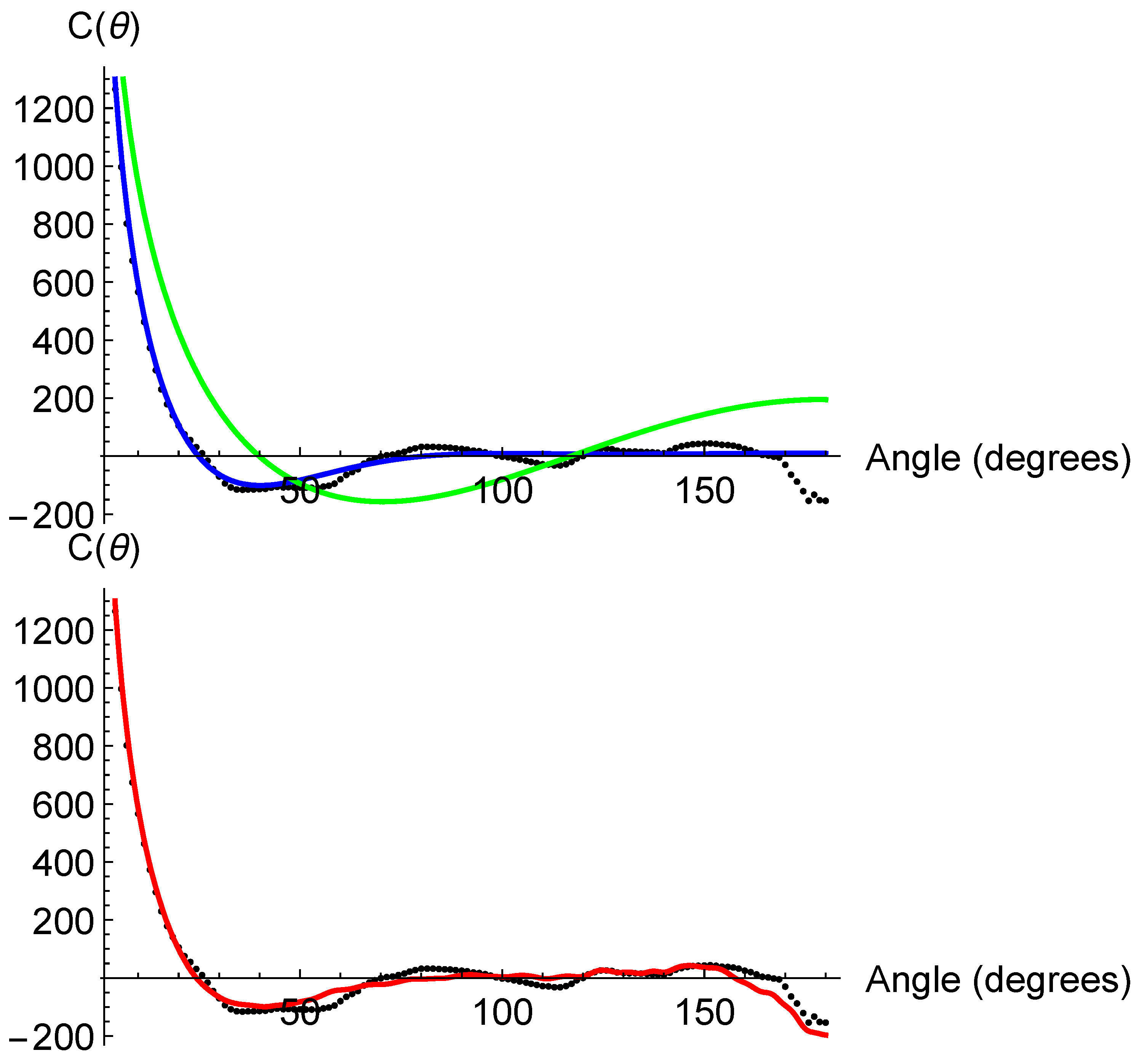
In ref. [22], the numerical interval $u_{\min }=4.5\pm 0.5$ was obtained from a best fit to the Planck 2018 dataset. In the upper panel of Figure 1, we plot $C\left(\theta \right)$ corresponding to the $\Lambda$CDM prediction ($u_{\min }=0$), together with the best fit to Planck data [17,18], as done in [23] with $u_{\min }=4.5$ but keeping even-odd parity balance. One can see at once that the standard cosmological model fails to fit the data, while the latter curve indeed yields almost zero correlations at $\simeq {70}^{\circ }$, but fails to reproduce the observed downward tail at $\sim {180}^{\circ }$. Finally, in the lower panel of Figure 1, we reproduce the excellent fit (${\chi }^2/\mathrm{d}.\mathrm{o}.\mathrm{f}.\approx 1$) performed in [22] to the same dataset requiring odd-parity dominance.

On the other hand, the maximum correlation angle ${\theta }_{\max }$ can be roughly estimated as

$${\theta }_{\max }\simeq \frac{{\lambda }_{\max }}{R_d}\to {\theta }_{\max }\simeq \frac{2\pi }{u_{\min }},$$

(8)

where $R_d=a\left(t_d\right)r_d$ stands for the proper distance from the LSS to us, and $u_{\min }=k_{\min }{r}_d$.

For later use, let us regroup the even and odd ℓ-multipoles in Equation (2), namely

$$\begin{array}{ccc}\hfill C\left(\theta \right)& =& C_{\mathrm{even}}\left(\theta \right)+C_{\mathrm{odd}}\left(\theta \right)=\hfill \\ & & \frac{1}{4\pi }\sum _{{\ell }_{\mathrm{even}}}(2\ell +1)C_{\ell }{P}_{\ell }(cos\theta )+\frac{1}{4\pi }\sum _{{\ell }_{\mathrm{odd}}}(2\ell +1)C_{\ell }{P}_{\ell }(cos\theta ).\hfill \end{array}$$

(9)

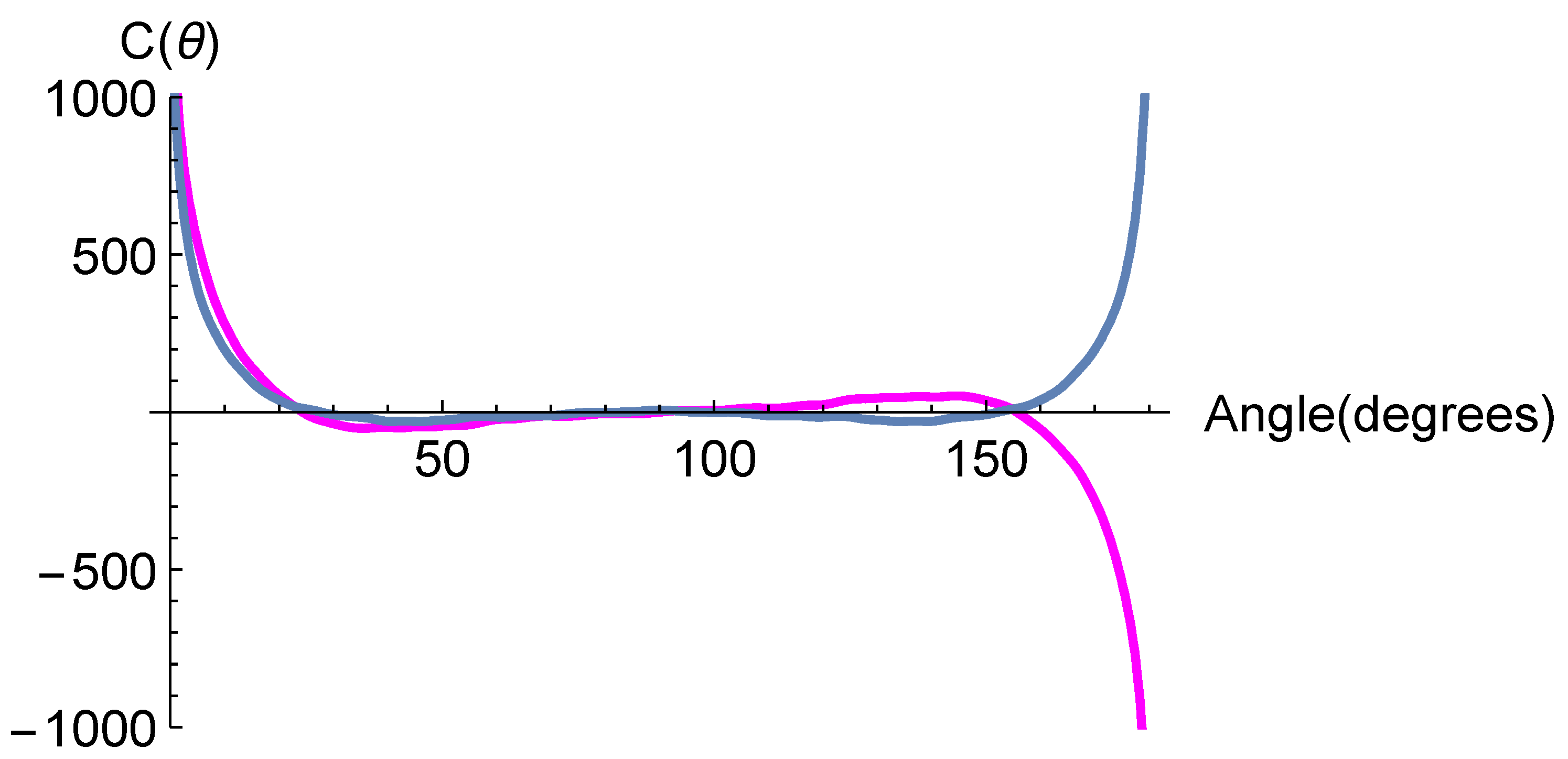
To better understand the behaviour of the $C\left(\theta \right)$ curve, we plot separately in Figure 2 the even and odd parity pieces $C_{\mathrm{even}}\left(\theta \right)$ and $C_{\mathrm{odd}}\left(\theta \right)$ as a function of $\theta$ for $\ell \in [2,401]$. Because of the oscillatory behaviour of the Legendre polynomials, both contributions add positively at small and middle angles, while a delicate balance is needed in order to obtain zero correlation at larger angles. This balance is indeed achieved [22] when using a single cutoff $u_{\min }$ in the evaluation of the $C_{\ell }$ coefficients in Equation (7).

However, if two distinct infrared cutoffs apply differently to even and odd ℓ-modes, such a delicate balance will be likely broken. Then, odd or even parity dominance can be obtained quite naturally. In the next section, we examine in depth this issue of paramount importance in this work.

4. Two Infrared Cutoffs in the CMB Power Spectrum

In ref. [22], the fit to Planck 2018 data was optimized using a $k_{\min }$ together with the requirement of parity imbalance by weighting adequately the odd and even terms in Equation (2). We shall now carry out a similar analysis but introducing two infrared cutoffs in the CMB power spectrum, namely, $k_{\min }^{\mathrm{even}}$ and $k_{\min }^{\mathrm{odd}}$, affecting the even- and odd-parity coefficients differently.

The goals of this new analysis are to provide: (i) a common explanation of both missing large-angle correlations and odd-parity dominance with fewer fitting parameters; and (ii) a physical interpretation behind. First, the numerical values of $k_{\min }^{\mathrm{even}}$ and $k_{\min }^{\mathrm{odd}}$ were heuristically determined from a fit of $C\left(\theta \right)$ to data, checking its consistency with odd-parity preference by means of a parity statistic to be discussed in Section 4.2. Depending on which $k_{\min }^{\mathrm{even}}$ or $k_{\min }^{\mathrm{odd}}$ is larger, odd or even dominance can be achieved.

On the one hand, the introduction of two infrared cutoffs in the angular power spectrum can be merely seen as a phenomenological approach to jointly account for missing large-angle correlations and the downwards tail in the $C\left(\theta \right)$ curve. Seen in this way, just an additional fitting parameter is required with respect to the analysis done in [23]. On the other hand, as we claim in this work, the ratio of both infrared cutoffs would become “fixed by theory” as a consequence of an extra (fermionic) spin degree of freedom due to the assumed fermionic nature of the underlying inflating field(s). Hence, no additional parameter is actually introduced into the fits.

Therefore, we compute separately the $C_{\ell }$ coefficients of the even and odd ℓ-multipoles according to

$$C_{{\ell }_{\mathrm{even}/\mathrm{odd}}}=N{\int }_{u_{\min }^{\mathrm{even}/\mathrm{odd}}}^{\infty }du\frac{j_{\ell }^2\left(u\right)}{u},$$

(10)

equivalent to Equation (7) for a single $k_{\min }$ without a distinction of parity. Now, the integral lower limits are: $u_{\min }^{\mathrm{even},\mathrm{odd}}=k_{\min }^{\mathrm{even},\mathrm{odd}}{r}_d$, respectively, where $r_d$ denotes again the distance from the LSS to us.

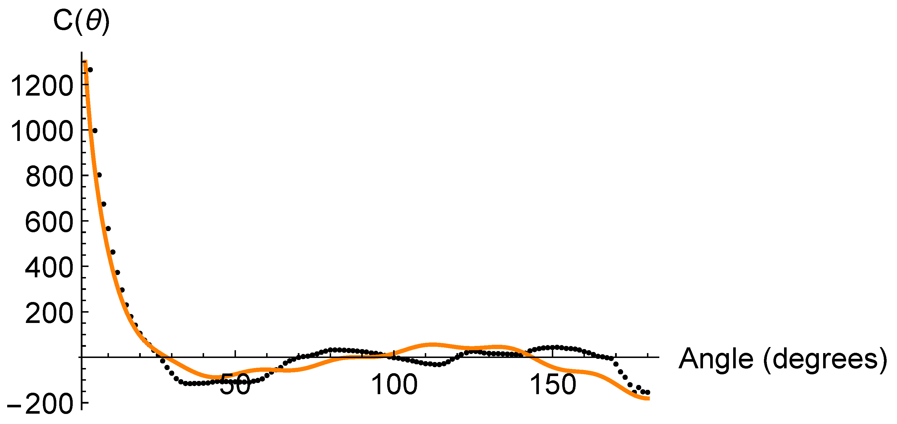
In Figure 3, we plot the fit of of $C\left(\theta \right)$ to Planck data under the assumption of two lower cutoffs $u_{\min }^{\mathrm{even},\mathrm{odd}}$ in the integral of Equation (7). From a best ${\chi }^2/\mathrm{d}.\mathrm{o}.\mathrm{f}.$ fit, we obtain $u_{\min }^{\mathrm{odd}}\simeq 2.67$ and, consequently, $u_{\min }^{\mathrm{even}}\simeq 5.34$. Admittedly, the new fit as seen in Figure 3 looks a bit worse than in the lower panel of Figure 1. However, notice that the number of free parameters is now smaller and, above all, one can simultaneously accommodate the lack of large-angle correlations and the apparent odd-parity dominance seen in the downward tail $\gtrsim {150}^{\circ }$, without resorting to any further fine-tuning of the $C_{\ell }$ coefficients.

Next, we estimate the statistical error of $u_{\min }^{\mathrm{odd}}$ (and $u_{\min }^{\mathrm{even}}=2u_{\min }^{\mathrm{odd}}$). As is well known, the $C\left(\theta \right)$ points are highly correlated, so that a calculation based on a simple ${\chi }_{\mathrm{d}.\mathrm{o}.\mathrm{f}.}^2$ procedure is not the most suitable. We circumvented this problem by using a Monte Carlo procedure similar to what was done in [22,23] to sample the variation of $C\left(\theta \right)$ within the measurement errors. To this end, we generated 100 mock CMB catalogs with bin size of $0.5^{\circ }$ each, corresponding to an ideal full sky case. Then, we computed the two-point correlation function $C_i\left(\theta \right)$ ($i=1,100$) in each realization. Next, we obtained $\Delta C_i\left(\theta \right)=C_i\left(\theta \right)-C_0\left(\theta \right)$, where $C_0\left(\theta \right)$ denotes the angular correlation function in standard cosmology. Defining $C\left(\theta \right)=C_{Planck}\left(\theta \right)+\Delta C_i\left(\theta \right)$, we computed $u_{\min ,i}^{\mathrm{odd}}$ from a best ${\chi }_{\mathrm{d}.\mathrm{o}.\mathrm{f}.}^2$ independent fit in each case, recalculating the $C_{\ell }$ coefficients and the respective normalization constant N of Equation (4). Let us mention that the latter shows an almost linear dependence (of negative slope) on the lower cutoff, namely, $N\in [340,180]$ versus $u_{\min }^{\mathrm{odd}}\in [2.36,2.98]$.

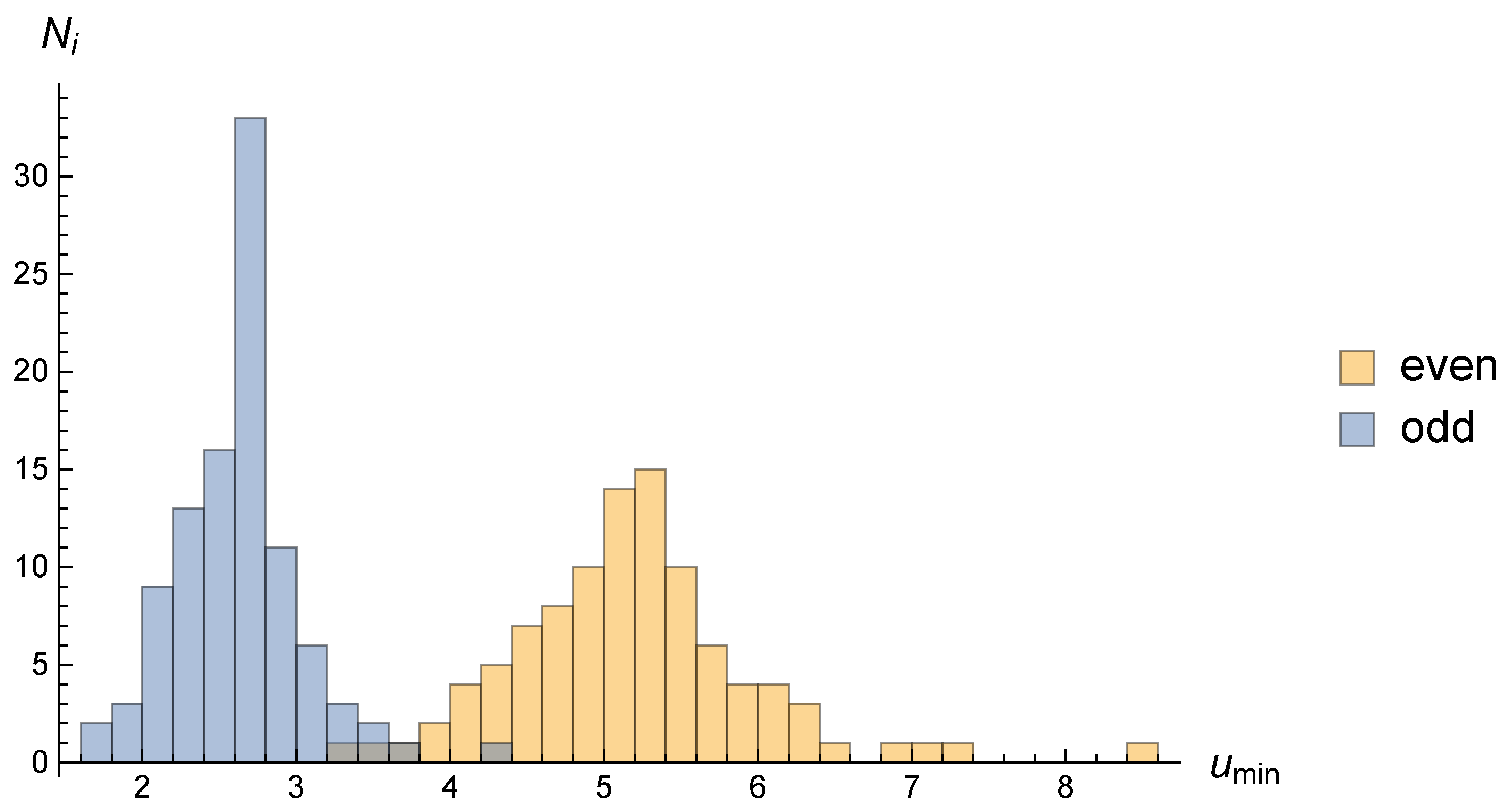
In Figure 4, we plot as a histogram the resulting $u_{\min ,i}^{\mathrm{odd}/\mathrm{even}}$ distribution(s) for all 100 realizations, both showing approximate Gaussian shapes. From these resulting roughly Gaussian distribution(s), we determined their average values and r.m.s., yielding

$$u_{\min }^{\mathrm{odd}}=2.67\pm 0.31;u_{\min }^{\mathrm{even}}=5.34\pm 0.62.$$

(11)

The above values imply non-zero values for $u_{\min }^{\mathrm{odd}/\mathrm{even}}$ corresponding to a $\simeq 8.6\sigma$ statistical significance in our analysis. Such a high confidence level reflects the need for two different lower cutoffs in the integral of Equation (10) for even and odd parity modes, in contrast to $\Lambda$CDM, to reproduce the angular correlation anomalies addressed in this work. As an aside, notice that the mean value of $u_{\min }^{\mathrm{even},\mathrm{odd}}$ lies within the interval $u_{\min }=4.5\pm 0.5$ found in [22] for a single lower cutoff, as naively expected.

Had we tried the opposite situation, $k_{\min }^{\mathrm{even}}<k_{\min }^{\mathrm{odd}}$, the $C\left(\theta \right)$ curve would have shown an upward tail, contrary to observational data. The mathematical reason why the condition $k_{\min }^{\mathrm{even}}>k_{\min }^{\mathrm{odd}}$ goes in the “right” direction is that the $C_{\ell }$ coefficients (for $\ell \lesssim 10$) decrease for ${\ell }_{\mathrm{odd}}$ to a lower extent than for ${\ell }_{\mathrm{even}}$ (as compared to no lower cutoff applied at all), thereby favoring odd-parity dominance, in accordance with observations. Let us note the greatest effect of the lower cutoffs affects $C_2$ and $C_3$ multipole coefficients (thereby decreasing the ratio $C_2/C_3$), while other low-ℓ modes also become modified (reduced), but to a lesser extent. This makes a difference with respect to, e.g., the ellipsoidal universe where only the quadrupole term is modified as compared to standard cosmology [32].

Next, notice the following relations between Legendre polynomials and the square of cosine functions with entire and half-entire (2$\pi$) periods (these relations can also be formulated in terms of Chebyshev polynomials [33]), called to play a fundamental role in our later development:

$$\begin{array}{ccc}\hfill P_1(cos\theta )& =& -1+2{cos}^2(\theta /2)\hfill \\ \hfill P_2(cos\theta )& =& -0.5+1.5{cos}^2\left(\theta \right)\hfill \\ \hfill P_3(cos\theta )& =& -1+0.75{cos}^2(\theta /2)+1.25{cos}^2(3\theta /2)\hfill \\ \hfill P_4(cos\theta )& =& -0.7184+0.6249{cos}^2\left(\theta \right)+1.0937{cos}^2\left(2\theta \right)\hfill \\ \hfill P_5(cos\theta )& =& -1+0.4687{cos}^2(\theta /2)+0.5469{cos}^2(3\theta /2)+0.9844{cos}^2(5\theta /2)\hfill \\ & \cdots & \hfill \end{array}$$

(12)

Higher order Legendre polynomials replicate the same pattern: besides a constant, even and odd Legendre polynomials either contain ${cos}^2\left[n\theta \right]$ or ${cos}^2\left[\right(n+1/2\left)\theta \right]$ terms, respectively. This pattern is just mathematical for the moment, below to be put in correspondence with the Fourier expansion of the constituents of a composite inflaton field, using a one-dimensional toy-model.

Inspired on very general grounds by superstring theory (obviously without entering at all in its complexity and intricacies [26,34]) and invoking a similar causality argument as employed for the single $k_{\min }$ case, we address now the possibility that any constituent (fermionic) field $\psi \left(\phi \right)$ (for simplicity, no more variables or indices are explicitly written) of a composite inflaton 3 satisfies either the periodic or antiperiodic boundary condition:

$$\begin{array}{ccc}\hfill \psi (\phi +2\pi )& =& \psi \left(\phi \right)\hfill \end{array}$$

(13)

$$\begin{array}{ccc}\hfill \psi (\phi +2\pi )& =& -\psi \left(\phi \right)\to \psi (\phi +4\pi )=\psi \left(\phi \right).\hfill \end{array}$$

(14)

The angular Fourier expansion of $\psi \left(\phi \right)$ for the periodic condition reads:

$$\psi \left(\phi \right)=\sum _{n\in \mathcal{Z}}{\alpha }_n{e}^{in\phi }$$

(15)

and for a real function,

$$\psi \left(\phi \right)=2\sum _{n\in {\mathcal{Z}}^{+}}\mathrm{Re}{\alpha }_n{e}^{in\phi },$$

(16)

so that only $cos\left(n\phi \right)$ terms appear in the Fourier expansion.

Let us define now a correlation function as in [36]

$${\int }_0^{2\pi }\psi \left(\phi \right)\psi (\phi +\Delta \phi )\frac{d\phi }{2\pi }.$$

(17)

For random Gaussian Fourier coefficients, if we define $\theta =\Delta \phi /2$, one finds

$$C(\Delta \phi )=2\sum _{n\in {\mathcal{Z}}^{+}}{C}_{n}cos(n\Delta \phi )\to C\left(\theta \right)=4\sum _{n\in {\mathcal{Z}}^{+}}{C}_n{cos}^2\left(n\theta \right)-2,$$

(18)

with $C_n=\langle {\alpha }_n{\alpha }_n^{*}\rangle$ and $\theta \in [0,\pi ]$ to be identified with the angle appearing as the argument of the two-point correlation function $C\left(\theta \right)$.

For the antiperiodic conditions, the Fourier expansion reads

$$\psi \left(\phi \right)=\sum _{n\in {\mathcal{Z}}^{+}+1/2}{\alpha }_n{e}^{in\phi },$$

(19)

which guarantees that it changes sign when $\phi \to \phi +2\pi$. Therefore,

$$C\left(\theta \right)=4\sum _{n\in {\mathcal{Z}}^{+}+1/2}{C}_n{cos}^2\left(n\theta \right)-2.$$

(20)

The above results obtained from this toy-model suggest the assignment of even- and odd-parity $C_{\mathrm{even}}\left(\theta \right)$ and $C_{\mathrm{odd}}\left(\theta \right)$ pieces in Equation (9), to fulfill the periodicity and antiperiodicity conditions given in Equations (12) and (13), respectively, somewhat recalling the well-known Ramond and Neveu–Schwarz sectors in superstring theory [26]. Hereafter, we shall assume that the above conclusions apply to the fundamental field(s) driving the expansion of the early universe.

4.1. Physical Interpretation

In the following, we will consider, without entering into details, the inflaton as an effective scalar field $\mathsf{\Phi }$ made out of two constituent fermionic fields ($\mathsf{\Phi }=\overline{\mathsf{\Psi }}\mathsf{\Psi }$) driving the expansion of the early universe. The causality condition yielding ${\lambda }_{\max }$ used for a single infrared cutoff is now assumed to split into two conditions applied independently to the periodic and the antiperiodic conditions in virtue of the spin degrees of freedom of the constituent fermionic fields of the effective inflaton.

Hence, in analogy to Equation (5), we shall now consider two maximum correlation lengths for even and odd parity multipoles, denoted as ${\lambda }_{\max }^{\mathrm{even}}$ and ${\lambda }_{\max }^{\mathrm{odd}}$, satisfying

$${\lambda }_{\max }^{\mathrm{even}}=2\pi R_h,{\lambda }_{\max }^{\mathrm{odd}}=4\pi R_h.$$

(21)

Then, two comoving wavenumbers $k_{\min }^{\mathrm{even}}$ and $k_{\min }^{\mathrm{odd}}$ can be defined from those length scales:

$$k_{\min }^{\mathrm{odd}}=2\pi a\left(t_d\right)/{\lambda }_{\max }^{\mathrm{odd}},k_{\min }^{\mathrm{even}}=2\pi a\left(t_d\right)/{\lambda }_{\max }^{\mathrm{even}}$$

(22)

corresponding to odd and even parity modes, respectively. Let us remark that physical momenta are given by $k/a\left(t\right)$, but the ratio $k_{\min }^{\mathrm{odd}}/k_{\min }^{\mathrm{even}}$ remains frozen after exiting the horizon. Note also that the numerical values of the lower cutoffs are obtained from a fit to correlation data and not from Equation (21). Indeed, what really matters in this work is that their ratio is equal (or close) to 2.

Moreover, two relevant angles can be defined following Equation (8) for a single $k_{\min }$:

$${\theta }_{\mathrm{even}}\simeq \frac{2\pi }{u_{\min }^{\mathrm{even}}}\simeq {65}^{\circ },{\theta }_{\mathrm{odd}}\simeq \frac{2\pi }{u_{\min }^{\mathrm{odd}}}\simeq {130}^{\circ },$$

(23)

defining three different angular intervals along the full 0${}^{\circ }$–180${}^{\circ }$ range, where the $C\left(\theta \right)$ function exhibits a different behavior, as can be easily appreciated in Figure 1 and Figure 3.

Now, from our discussion in the previous section on the Fourier expansion of $C\left(\theta \right)$, we will take into account that the $C_{\mathrm{even}}\left(\theta \right)$ and $C_{\mathrm{odd}}\left(\theta \right)$ pieces of Equation (9) can be associated with terms of the type ${cos}^2\left[n\theta \right]$ and ${cos}^2\left[\right(n+1/2\left)\theta \right]$, respectively, as shown in Equation (12). Therefore, the two distinct lower limits $u_{\min }^{\mathrm{even},\mathrm{odd}}$ for even and odd multipoles in the integral of Equation (4) can be related to the infrared cutoffs $k_{\min }^{\mathrm{even},\mathrm{odd}}$, respectively.

Moreover, from the fit to Planck data shown in Figure 3, the ratio $u_{\min }^{\mathrm{even}}/u_{\min }^{\mathrm{odd}}=k_{\min }^{\mathrm{even}}/k_{\min }^{\mathrm{odd}}$ turns out to be quite close to 2. This phenomenological fact may be further understood by considering the periodicity and antiperiodicity conditions applied to the maximum correlation lengths:

$$\frac{u_{\min }^{\mathrm{even}}}{u_{\min }^{\mathrm{odd}}}=\frac{k_{\min }^{\mathrm{even}}}{k_{\min }^{\mathrm{odd}}}=\frac{{\lambda }_{\max }^{\mathrm{odd}}}{{\lambda }_{\max }^{\mathrm{even}}}=2,$$

(24)

as implied by Equation (21). In the framework of the $R_h=ct$ universe, this relation corresponds to two different exit times of the Planck regime: first the $k_{\min }^{\mathrm{odd}}$ mode and later the $k_{\min }^{\mathrm{even}}$ mode. In the usual inflationary scenario, it implies again two different times in similar order but exiting the Hubble horizon. Needless to say, the above ratio 2 is expected to be valid only approximately, but it has been exactly to this value in our numerical analysis.

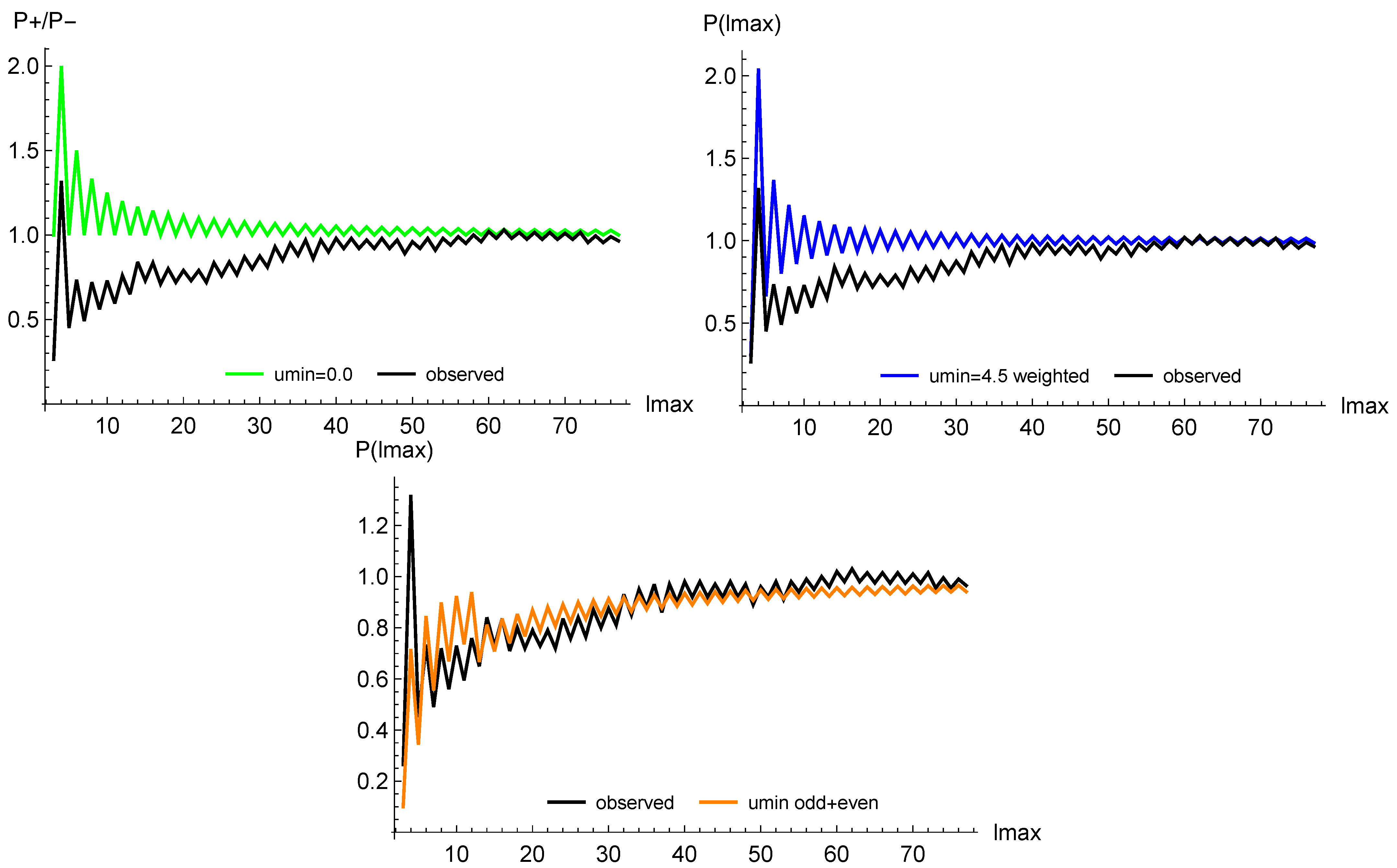
4.2. Parity Statistic Study

Let us now address the deviation from the even-odd parity balance employing the parity statistic [19,20], as done in [22]

$$P\left({\ell }_{\max }\right)=\frac{P^{+}\left({\ell }_{\max }\right)}{P^{-}\left({\ell }_{\max }\right)};P^{\pm }\left({\ell }_{\max }\right)=\sum _{\ell =2}^{{\ell }_{\max }}{\gamma }_{\ell }^{\pm }\frac{\ell (\ell +1)}{2\pi }{C}_{\ell },$$

(25)

with the projectors defined as ${\gamma }_{\ell }^{+}={cos}^2(\ell \pi /2)$ and ${\gamma }_{\ell }^{-}={sin}^2(\ell \pi /2)$. Assuming that $\ell (\ell +1)C_{\ell }\sim \mathrm{constant}$ is satisfied at low ℓ, $P^{\pm }$ can clearly be considered as a measurement of the degree of parity asymmetry. Any deviation from unity of this statistic points to an even-odd parity imbalance: below unity, it implies odd-parity dominance and vice versa. Below, we apply this statistic to compare different fits with one or two infrared cutoffs.

In Figure 5, we plot $P\left({\ell }_{\max }\right)$ as a function of ${\ell }_{\max }$ corresponding to (a) upper panel: $u_{\min }=0$ (expected from $\Lambda$CDM); (b) our previous result for $u_{\min }=4.5$ and odd-parity dominance [22]; (c) the new analysis performed in this paper setting $u_{\min }^{\mathrm{even}}=2u_{\min }^{\mathrm{odd}}\simeq 5.34$, as obtained before. From inspection of these plots it becomes apparent that the fit using a $k_{\min }^{\mathrm{odd},\mathrm{even}}$ pair somewhat worsens with respect to the single $k_{\min }\ne 0$ case: the reduced ${\chi }^2/\mathrm{d}.\mathrm{o}.\mathrm{f}.$ increases from almost unity to about twice. Nonetheless, as already emphasized, the main interest of providing a common explanation to both missing large-angle correlations and odd-parity dominance, remains.

5. Discussion and Conclusions

As claimed in ref. [23], the lack of large-angle correlations observed in the CMB from WMAP and Planck 2018 data can be reproduced, introducing a lower cutoff $k_{min}$ to the CMB power spectrum, thereby implying a lower $u_{min}$ in the computation of all (even and odd) $C_{\ell }$ coefficients of the multipole expansion in Equation (4). Furthermore, the apparent odd-parity dominance manifesting as a downward tail of $C\left(\theta \right)$ at large angles ($\theta \gtrsim {150}^{\circ }$), but keeping the good behaviour at lower angles, can also be accommodated thanks to ad hoc extra weights of the multipole coefficients $C_{\ell }$ ($\ell \lesssim 10$), leading at the same time to an excellent fit of the parity statistic $P\left({\ell }_{\max }\right)$ [22].

No obvious theoretical connection between such an infrared cutoff $k_{\min }$ (i.e., lack of large-angle correlations) in the power spectrum and parity imbalance has been found so far [21,22,37,38]. In this paper, however, we put forward a possible relationship between both by introducing two infrared cutoffs $k_{\min }^{\mathrm{even}}$ and $k_{\min }^{\mathrm{odd}}$, whose ratio is close to 2 from a ${\chi }_{\mathrm{d}.\mathrm{o}.\mathrm{f}.}^2$ best fit to Planck 2018 data. In this way we are able: (i) to reduce the number of fitting parameters with respect to [22], while reproducing the downward tail at large angle; (ii) to provide a theoretical connection (without resorting to any particular model) between both observations, setting the ratio $k_{\min }^{\mathrm{even}}/k_{\min }^{\mathrm{odd}}=u_{\min }^{\mathrm{even}}/u_{\min }^{\mathrm{odd}}$ exactly equal to 2.

Thus, new fits of $C\left(\theta \right)$ and the parity statistic $P\left({\ell }_{\max }\right)$ have been performed using the same Planck 2018 data set as for the single infrared cutoff case [22]. Since the number of fitting parameters is now considerably smaller, the goodness of the fits (determined by their ${\chi }^2/\mathrm{d}.\mathrm{o}.\mathrm{f}.$) somewhat worsens. However, let us emphasize the added value of our approach due to a common and suggestive explanation of both anomalies: missing correlations above 60${}^{\circ }$–70${}^{\circ }$ and a downward tail at ≳150${}^{\circ }$, based on a suggestive physical interpretation.

For the numerical computations of the lower cutoffs and their associated errors, a Monte Carlo procedure was employed generating 100 mock CMB maps to sample the variation of $C\left(\theta \right)$ within the measurement uncertainties, yielding

$$u_{\min }^{\mathrm{odd}}=2.67\pm 0.31;u_{\min }^{\mathrm{even}}=5.34\pm 0.62,$$

(26)

corresponding to a $8.6\sigma$ statistical significance of our working hypothesis. The need for non-zero lower cutoffs $u_{\min }^{\mathrm{odd}/\mathrm{even}}$ (in contrast to $\Lambda$CDM) to reproduce the anomalies of angular correlations examined in this paper has to be interpreted with care within our phenomenological approach.

On the other hand, based on a Fourier analysis and using a toy-model, we have associated even and odd multipoles of $C\left(\theta \right)$ with periodic and antiperiodic boundary conditions satisfied by the underlying (fermionic fields) of a composite inflaton, or a fermionic inflaton itself. Thus, the phenomenologically motivated choice for the ratio $k_{\min }^{\mathrm{even}}/k_{\min }^{\mathrm{odd}}$ becomes supported by theoretical arguments based on spin, beyond the initial heuristic approach. This constitutes the main result of this work.

As is well known, spin degrees of freedom play a crucial role in elementary particle physics, e.g., predicting the gyromagnetic ratio g for the self-spinning electron to be about two times bigger than the value for an orbiting electron [39]. Needless to say, the famous muon $g-2$ deviation from zero stands as an important test of new physics, currently under close scrutiny [40]. The idea of searching for new physics and phenomena either at particle colliders on Earth and/or looking at the sky, in a complementary way, is certainly not new, with dark matter being a good example of it.

Of course, explanations alternative to ours for missing large-angle correlations together with odd-parity dominance are possible: a statistical fluke of data at large angles, contamination or non-cosmological effects [41,42], cosmic variance [43], or even other theoretical underlying reasons.

Finally, let us point out that the future very-high precision measurements of CMB polarization [44,45,46], might follow (or not) an angular pattern similar to the temperature fluctuations seen in the sky, thereby shedding light on this tantalizing hypothesis.