Article

The Hubble Diagram: Jump from Supernovae to Gamma-ray Bursts

by
Nikita Yu. Lovyagin
1,*,†,
Rustam I. Gainutdinov
2,3,†,
Stanislav I. Shirokov
3,† and
Vladimir L. Gorokhov
4,†
1
Department of Computer Science, Saint Petersburg State University, 7/9 Universitetskaya Nab., St. Petersburg 199034, Russia
2
Department of Astrophysics, Saint Petersburg State University, 7/9 Universitetskaya Nab., St. Petersburg 199034, Russia
3
Saint Petersburg Branch of Special Astrophysical Observatory, Russian Academy of Sciences, 65 Pulkovskoye Shosse, St. Petersburg 196140, Russia
4
Innovation Management Department, Saint Petersburg Electrotechnical Univeristy, Ulitsa Professora Popova 5, St. Petersburg 197376, Russia
*
Author to whom correspondence should be addressed.
These authors contributed equally to this work.
Universe 2022, 8(7), 344; https://doi.org/10.3390/universe8070344
Submission received: 28 March 2022 / Revised: 18 June 2022 / Accepted: 21 June 2022 / Published: 23 June 2022
(This article belongs to the Special Issue Supernovae as Cosmological Probes)

Abstract

:
The Hubble diagram (HD) is a plot that contains a luminous distance modulus presented with respect to the redshift. The distance modulus–redshift relation of the most well-known “standard candles”, the type Ia supernovae (SN), is a crucial tool in cosmological model testing. In this work, we use the SN Ia data from the Pantheon catalogue to calibrate the Swift long gamma-ray bursts (LGRBs) as “standard candles” via the Amati relation. Thus, we expand the HD from supernovae to the area of the Swift LGRBs up to z 8 . To improve the quality of estimation of the parameters and their errors, we implement the Monte-Carlo uncertainty propagation method. We also compare the results of estimation of the Amati parameters calibrated by the SN Ia, and by the standard ΛCDM model and find no statistically significant distinction between them. Although the size of our LGRB sample is relatively small and the errors are high, we find this approach of expanding the cosmological distance scale promising for future cosmological tests.

1. Introduction

The Hubble diagram (HD) is a plot of object redshifts z with respect to object distances d. The HD is a well-known and widely used practical cosmological test [1,2,3]. Based on cosmological models, one usually describes the theoretical redshift–distance relation as a parametric function d ( z , p ) , where p is a parameter vector. Thus, the cosmology-independent determination of distances to objects with known redshift gives one a unique opportunity to verify, compare and probe parameters of cosmological models. In the case of the standard ΛCDM cosmological model, for the HD, p may be considered, for example, as  ( H 0 , Ω M ) .
Usually, the HD is built up using the so-called standard candles (SC), i.e., the objects with theoretically or empirically known absolute brightness (or magnitude). Measured visible magnitudes of SCs directly give one required distances. At the end of the 20th century, the HD was constructed for type Ia supernovae (SNe Ia) standard candles. Thus, the accelerated expansion of Universe within the standard Friedmann–Lemaitre–Robertson–Walker (FLRW) [2] cosmological model was discovered. This led to the introduction of dark energy into the standard cosmological model (SCM) [4,5]. However, there is still a wide discussion on cosmological models and their parameter values [6,7,8,9]. The wCDM model, where the ΛCDM model is a special case of one, is often considered an alternative to SCM. The wCDM model is defined as the FLRW model that contains two cosmological non-interacting fluids, having an equation of state of cold matter p = 0, and the quintessence (dark energy) p = w ρ c 2 (with w < 0 ) [2].
The current limit of SN observations is about z 2–3, while the long gamma-ray bursts (LGRBs) up to z 10 are already seen [10,11]. This makes them promising objects to prolong the HD significantly further into the Universe. The LGRB sources are related to explosions of massive core-collapse SN in distant galaxies [12], though up to now, there is no satisfactory theory of the LGRB radiation origins [13,14]. There are a number of studies that suggest using LGRBs as SCs [15,16,17,18,19,20,21,22,23,24,25]. We suppose that LGRB HD can be used for probing cosmological parameters p and comparing cosmological models, as well as the SN HD [3,26,27].
The Amati relation is an observed linear-like correlation between LGRB spectrum parameters, including redshift and distance to LGRB host galaxy, in the logarithmic plot [18]. Despite the fact that individual LGRBs may not satisfy the Amati relation due to both physical and observational factors, we expect that for a statistically large ensemble of LGRBs, the correlation is correct on average. So the relation gives one a statistical opportunity to measure the distance to LGRBs with known redshift independently of a cosmological model. However, it depends on two unknown parameters that have to be calibrated observationally. For calibration of the correlation, the LGRBs with known distances and redshifts are needed, so the first step of our study is in determining distances d for a subsample of LGRBs in near galaxies by cosmology-independent methods.
In this study, we try to calibrate the Swift LGRBs (https://swift.gsfc.nasa.gov/archive/grb_table/ (accessed on 12 January 2022)) as standard candles by using ΛCDM as a basis, i.e., obtaining distances from the model. However, this approach involves the circularity problem [28] as, for the proper calibration of the cosmologically independent distance, the measurement that should be used. So next, we calibrate LGRBs as standard candles by using the Pantheon SNe Ia [29] as a basis.
We decided to approximate the SN HD by using a smooth elementary mathematical function d S N ( z ) that can be directly used to obtain the distances to sources of LGRBs with known z. The LGRBs should be near enough so that they can lie inside representative SN sample, where the distance error σ d S N ( z ) is small enough. Corresponding cosmological background of the Amati relation and introduction in mathematical approach of its calibration was described in [3]. In that article, the LGRB sample calibrated by Amati via globular clusters [19] was used to construct the Hubble diagram, and the calibration method for supernovae was also described. In the current article, we use a specially selected LGRB sample, a modified supernova calibration method (by improved formula), and more advanced statistical methods: the Monte-Carlo uncertainty propagation to account for errors and the Theil–Sen estimator to find the best-fit parameters. Thus, in this work, we obtain a new estimation of values of the Amati parameters and of the LGRB Hubble diagram.
The second step is in determining the Amati relation parameters via selected near LGRBs (i.e., LGRB calibrating), finding distances to all LGRBs with known redshift via the calibrated Amati relation, and plotting the HD for them. In fact, SNe are also calibrated SCs via cepheids that are also calibrated (via parallaxes) such that our approach lies in the frameworks of extending the cosmological distance scale. Since the supernova catalogue data are tied to a fixed value of the Hubble constant H 0 = 70 km/s/Mpc, this approach is not completely cosmologically independent, and all values are obtained with an accuracy of the scale factor H 0  [30].
At almost every stage of this study, it is required to find the best-fitting parameter estimation. In case, for example, of the Amati parameters, the best-fitting function y = f ( x ) should take into account errors in data points both of x and y. Because of this and the lack of LGRB statistics, we find the common linear least-square method to be unsuitable for our study. Instead we use the Theil–Sen estimator (also known as the single median method) for the linear regression purposes [31]. In this method, the estimation for the slope is defined as the median slope among all of the possible pairs of dots. We also need a method to perform the parameter estimation (the curve fitting) routines for the arbitrary function f. For this, we use the trust region reflective algorithm [32], which is the non-linear least-squares method implemented in the curve_fit function of the scipy.optimize Python library [33]. We can interpret both of these methods as pipelines that return the estimated parameters based on the input data. Our purpose is to also estimate the errors and covariances of the parameters. To do this, we utilise the Monte-Carlo sampling uncertainty propagation approach [34,35]. Applied to our pipelines, this approach allows us to correctly propagate the errors directly from the input data to the estimated parameters.
In the paper, we calibrated the LGRBs from the specially selected Swift subsample as SCs via supernovae, as it is described above, and built the corresponding LGRB HD, which is the main result of this work. Nowadays, there are still not enough statistics and theory to obtain reliable values of cosmological parameters from the LGRB HD. However, we find our method promising. We also compare ΛCDM-based and SN-based Amati parameters and find no significant difference between them.

2. Materials and Methods

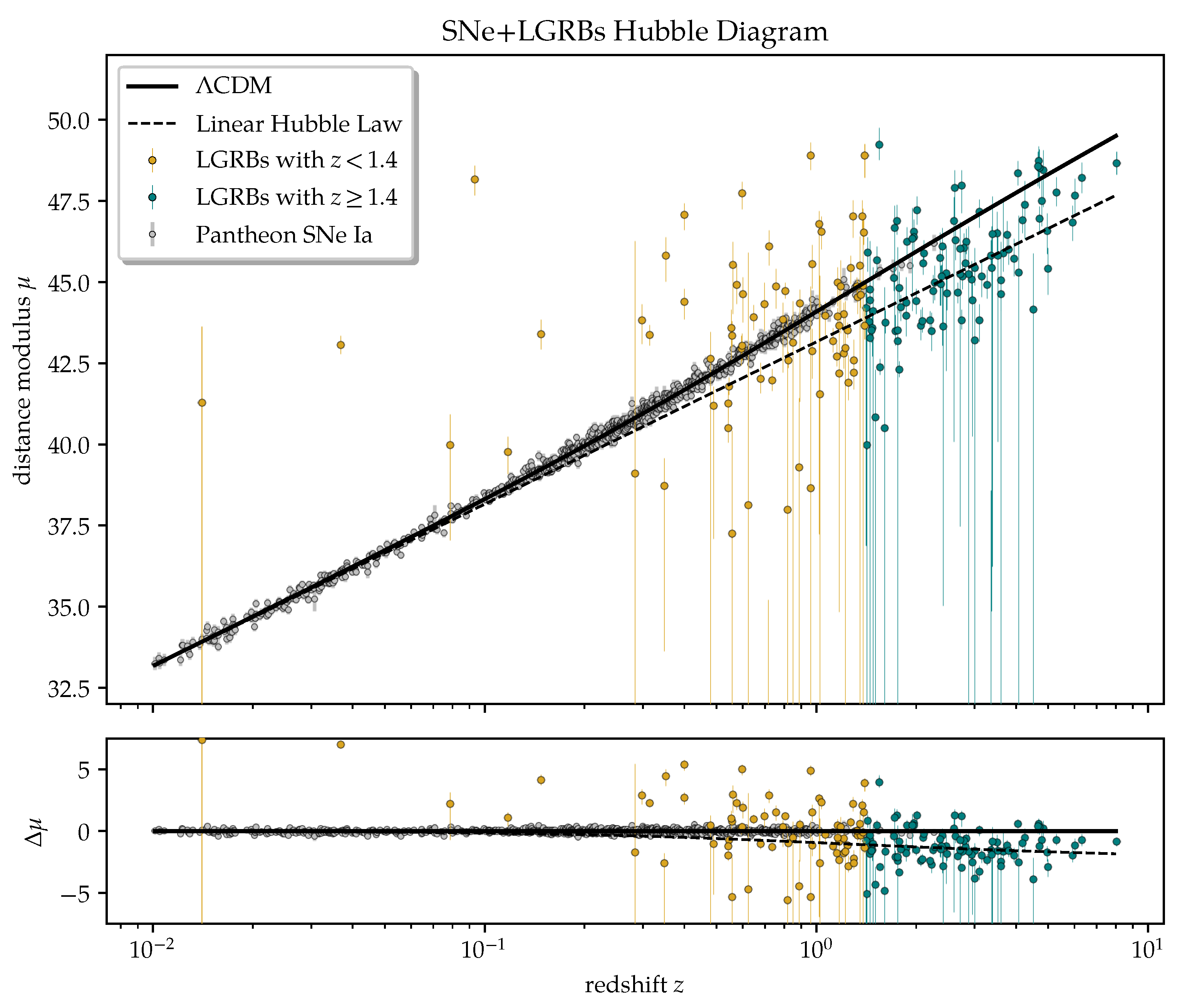
2.1. The Hubble Diagram as a Basic Cosmological Test

The HD is the redshift–distance relation, which can be represented as a table of points ( z i , d i ) on the plot for each i-th object. Usually, the luminosity distance d L is used. This value depends on the visible magnitude m, absolute magnitude M, and distance modulus μ as
m M = μ = 5 log ( d L / 1 Mpc ) + 25 .
In fact, a HD plots the ( z i , μ i ) relation.
In general, cosmological models give theoretical assumptions on the function d L ( z , p ) , where p are model parameters. For example, in wCMD model p = { H 0 , w , Ω w , Ω k } , and in ΛCMD model p = { H 0 , w = 1 , Ω w = Ω Λ , Ω k = 0.0 } . The HD is one of the cosmological tests that allow one to find the model parameters via fitting the observational data. For this one, the redshift z and distance d L should be determined independently (e.g., z directly via spectrum, and  d L via various indirect methods).

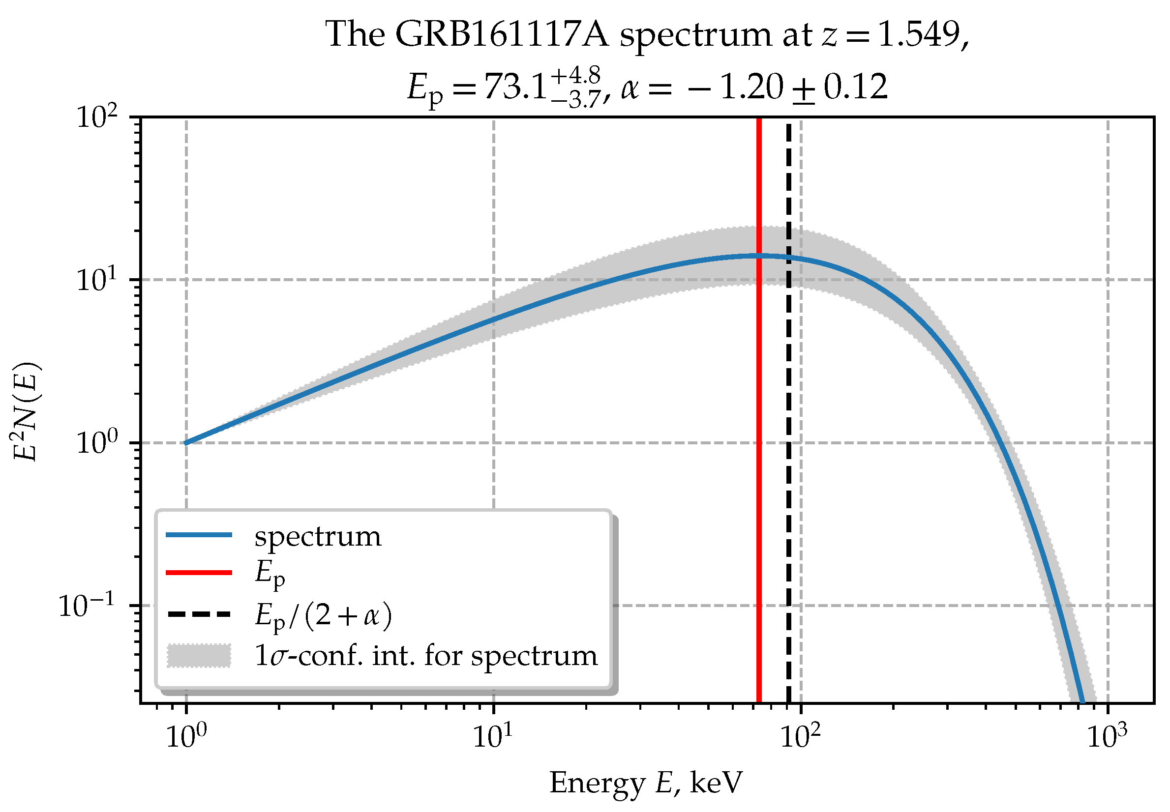
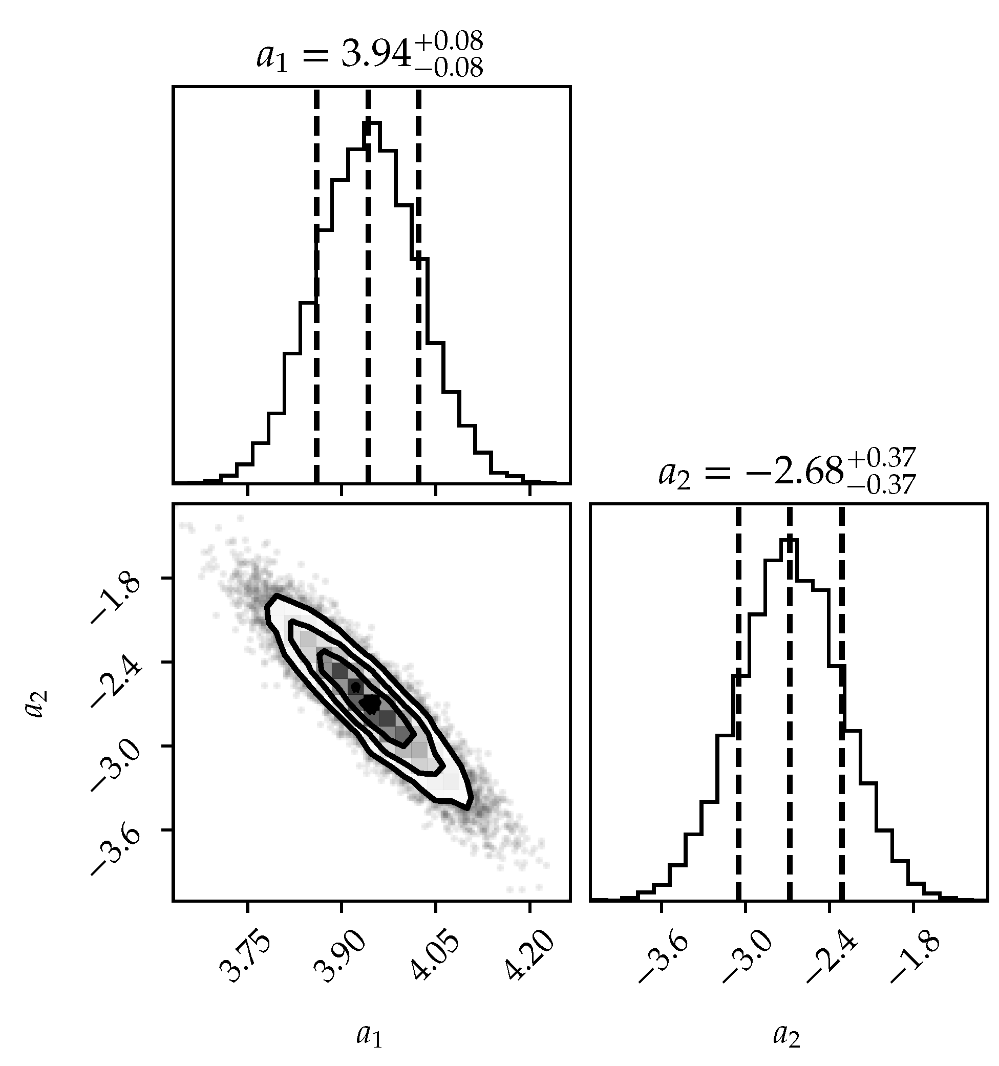
2.2. Gamma-ray Bursts as Standard Candles

Standard candles are a group of objects with the known (theoretically or empirically) typical absolute magnitude M. They allow one to find the luminosity distance or distance modulus directly from Equation (1) by using the visible magnitude m, or bolometric fluxes.
In the case of LGRBs, the situation is a little different. The Amati relation for LGRBs [15,18,19] is the equation
log E iso = a log E p , i + b ,
where
  • E p , i = E p ( 1 + z ) is the rest frame spectral peak energy, where E p is the observed spectrum peak energy;
  • E iso = 4 π d L 2 · S bolo / ( 1 + z ) is the isotropic equivalent radiated energy in gamma-rays [36]. The distance d L and observed integral fluence S bolo are determined as quantities transferred per a unit energy frame area and that are corrected for the instrumental (observed) spectral energy range, and source redshift. The correction is performed by the equation
    S bolo = S obs 1 1 + z 10 4 1 + z E N ( E ) d E E min E max E N ( E ) d E ,
    where S obs is the observed fluence, and  { E min , E max } is the instrumental spectral energy range, which is { 15 , 150 } keV for the Swift’s BAT instrument;
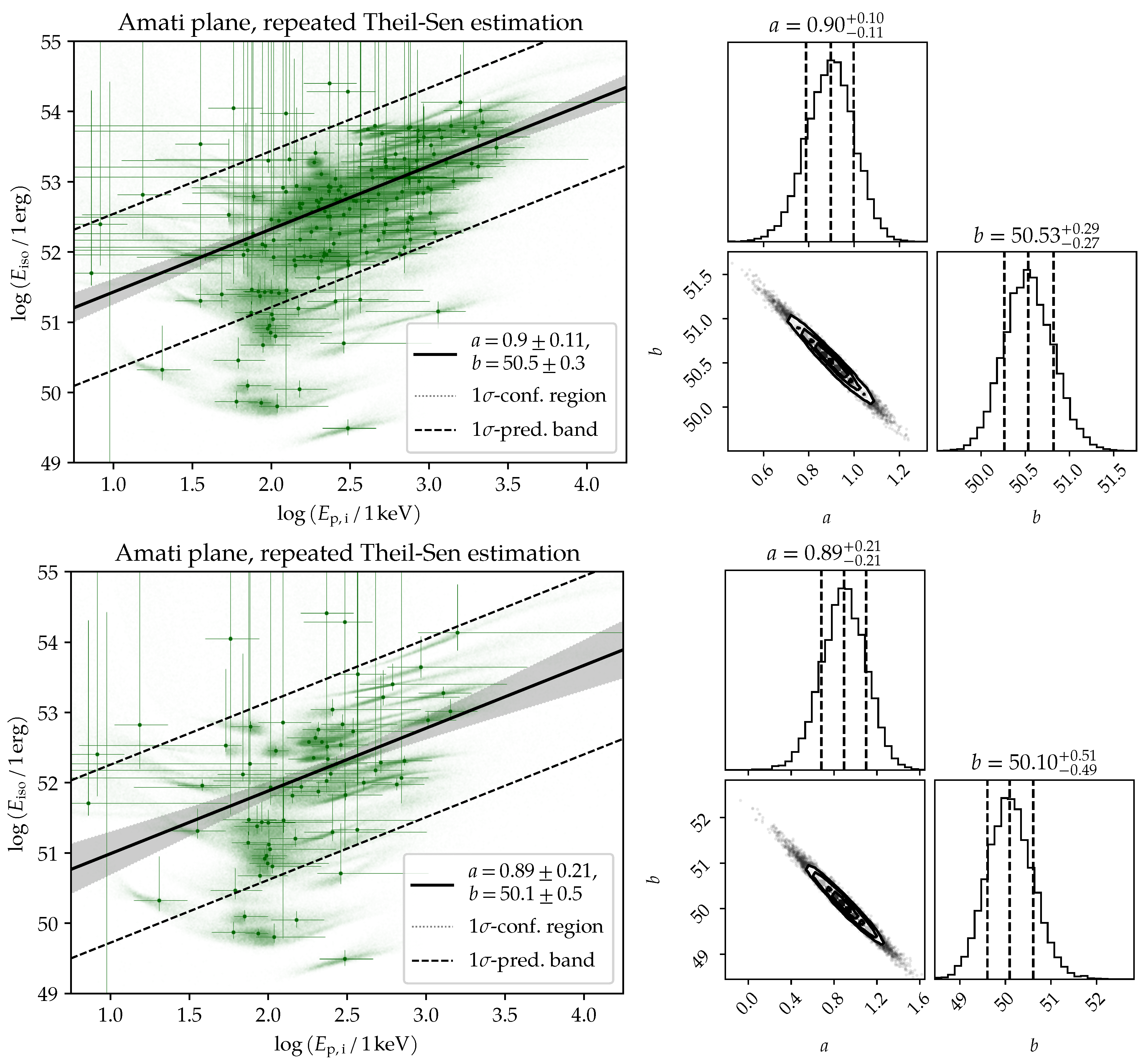
  • a and b are the Amati relation parameters mentioned above that can be calibrated empirically as in this study.
If observed parameters z, S bolo , E p , i , and model-independent measurement of d L ( z ) (at the small scales z 1.5 ) are known, then the best fit of the Amati relation parameters a and b can be found. Using a, b, z, S bolo , and  E p , i , one can find the LGRB distances d L LGRB ( z ) via the Amati relation and plot the LGRB HD.
The value of E p is usually determined via fitting the LGRB spectrum by the Band model [37]. However, the Swift database contains values of E p determined via fitting the spectrum by a cut-off power law (CPL) model function N ( E ) ,
N ( E ) photons KeV s cm 2 = A E α exp ( 2 + α ) E / E p ,
where α and E p are the CPL model best-fit parameters of an LGRB. A normalized example of the CPL model (energy spectrum, E 2 N ( E ) , that has its maximum at E p ) is shown in Figure 1. Although the result of determining the peak energy of the spectrum may differ for different spectrum fitting function choices, we expect that this difference will not significantly affect the linear correlation of log E p , i and log E iso . We find the Swift database sample containing the values of E p , estimated via the CPL model, to be more representative and suitable in our current study in the sense of measurement error equality, as obtained on a single instrument.
So, to find a and b, one needs to obtain the luminosity distances d L for near LGRBs. Although taking d L ( z ) from the ΛCMD model or from any other cosmological model is a dead-loop (a circularity problem), we have first calibrated a and b using ΛCMD model using parameters from [6] as a comparison basis.
Then, we chose the way of the SN calibration. Thus, we attempted to build a function d L SN ( z ) by using SNe Ia as SCs. Distance d L was calculated as function d L SN ( z ) for near LGRBs that have redshifts z low enough in order to perform an interpolation of the SN HD.
This lets one directly obtain the Amati relation parameters and use them for cosmological model-independent determination of distances d L to all LGRBs with known observational data for z, S bolo , and E p , i and to plot the HD for them.

2.3. Catalogues of SNe Ia and LGRBs

We used the Pantheon database (containing 1048 SNe). In this catalogue, there are two kinds of redshift, which are the redshift in terms of the cosmic microwave background radiation z cmb , and the redshift in terms of the heliocentric system z hel [29]. Between these two methods, we chose the z cmb one. All the catalogue data are calculated in assumption of H 0 = 70 km/s/Mpc, so we set this value throughout our study.
For our purposes, we use the sample of 174 GRBs from the Swift catalogue with the measured parameters of ( α , E p , S obs , z ) , where the spectral parameter α , the peak energy E p , and the observed flux S obs are described above, and z is the redshift. Some of the uncertainties of these parameters were missing (several α errors and approximately a third of E p errors were not presented). To deal with this issue, we assume the points with unknown errors to have the relative uncertainties equal to the median relative uncertainties of the corresponding parameter of the sample. The redshift z values are also presented in the lack of uncertainties, as is expected. A significant proportion of the LGRB parameters has asymmetric and relatively huge errors, which leads to the inexpediency of using the common uncertainty propagation rule. Instead, we use the approach of Monte-Carlo sampling, which is thoroughly described in Section 2.4.

2.4. Monte-Carlo Uncertainty Propagation

The standard approach to the error propagation problem is known as the linear uncertainty propagation (LUP) theory. One of the best implemented error propagation software is the uncertainties package of the Python language. The errors in this approach are interpreted as the standard deviations, while the values have the sense of the mean. So, the values of variable with their error are defined by the normal distribution, which denotes the possible whereabouts of the variable via distribution parameters. However, the LUP theory requires that the errors be relatively small compared to the values of variable so that the functions in calculations are nearly linear compared to these small shifts. Additionally, the LUP approach is not capable of handling asymmetric errors. Thus, we cannot use it.
For that reason, we decided to use the Monte-Carlo sampling. In this approach, the values and their errors also have the sense of defining the distributions of possible locations, and we used these distributions to draw samples of the size of 10,000. To handle the asymmetric uncertainties, we interpreted the values as the medians, the lower bounds were interpreted as the 0.16 quantiles, and the upper bounds as the 0.84 quantiles. With this interpretation of errors, the case of symmetric uncertainties reduces to the normal distribution with the known mean and standard deviation. In the case of asymmetric errors, we used the split-normal distribution, which results from joining the two halves of normal distributions with different standard deviations at their mode. Some of the E p values from our LGRB data set had remarkably huge lower uncertainties such that trying to Monte-Carlo sample them would lead to negative E p values, which has absolutely no physical sense. Because of that, in the case of E p variables, we drew the split-normal distributions in the space of log E p . So, the peak energy values were drawn using the log-split-normal distributions. Taking the logarithms does not move the quantiles, so the errors in this case are not changed.
The Monte-Carlo approach to propagating the errors is simple yet powerful. It allows one not only to calculate the uncertainties of calculated values, but also to track and take into account the correlations between variables for free.

2.5. Best-Fitting Methods

To obtain the best-fit parameters of the approximation function d L S N ( z ) for the SN HD, one needs to minimise the functional value
χ 2 = i = 1 n 1 σ i 2 y i f ( x i , p ) 2 ,
where
  • ( x i , y i ) are observed table values;
  • σ i is error of i-th value;
  • f is the model function and p = { p 1 , p 2 , , p m } are the parameters.
This function utilises the trust region reflective algorithm [32] to minimise the χ 2 function.

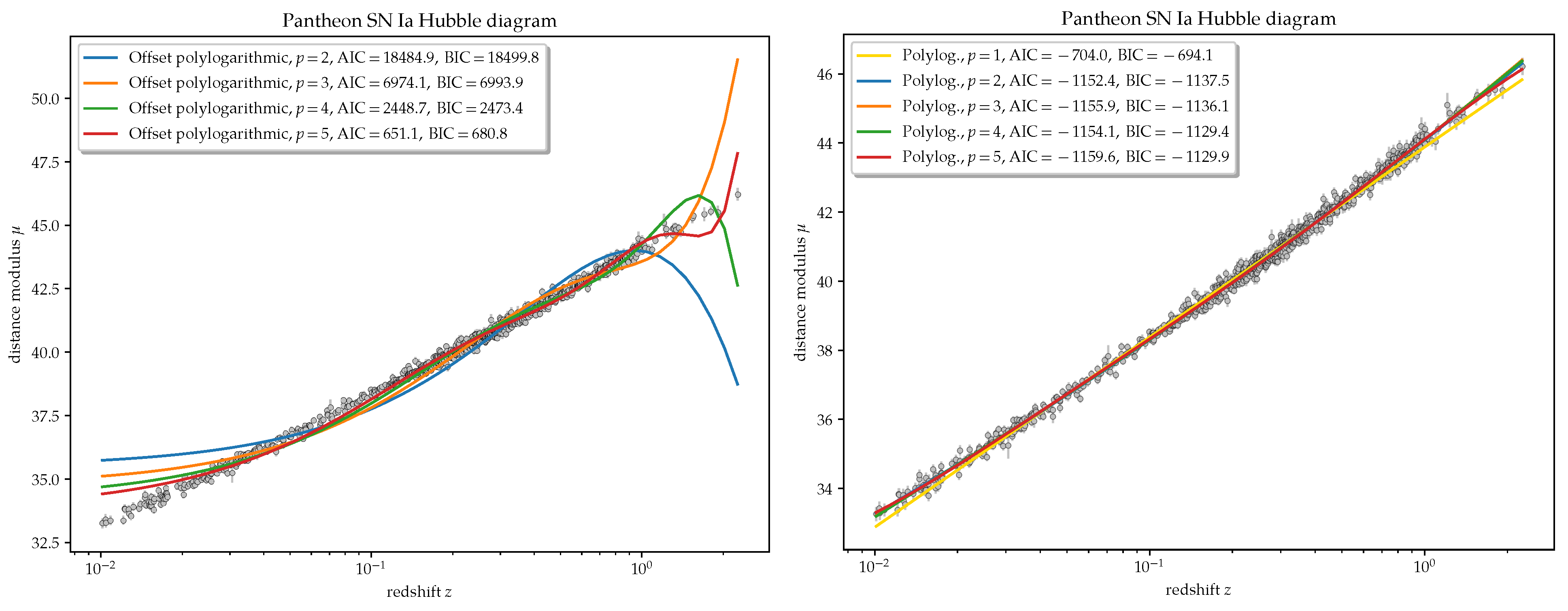
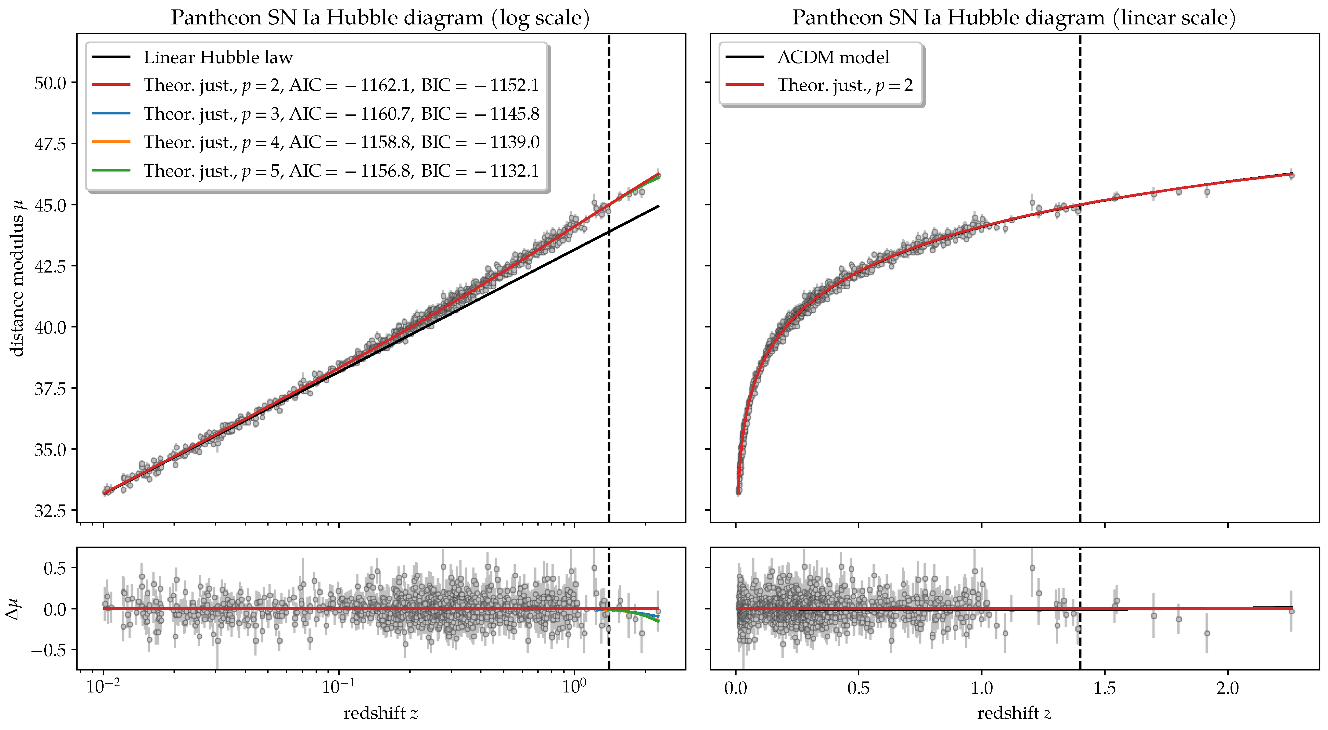
2.6. Interpolation Function of the SN HD

In fact, we can use any smooth function to use it as a d L S N ( z ) function. All that we need in order to minimise the error between the real value and a mathematically predicted one for the luminous distance at any low z, where we have enough supernovae to do this, is the approximation accuracy that is provided by our approach in the redshifts z m i n z z m a x , where z m i n and z m a x are redshifts of the nearest and the farthest supernovae ( z = 0.01012 and z 2.26 , respectively).
Since in logarithmic scales (along both of the distance and redshift) the relation d L ( z ) is already known, and it has almost a linear behaviour at low z, we decided to use a polylogarithmic function of a degree k. We tried to use the three following functions:
  • Theoretically-inspired function
    μ S N ( z ) = 5 log c z H 0 + 25 + i = 1 p a i log i ( 1 + z ) ;
  • Simple polylogarithmic function
    μ S N ( z ) = i = 0 p a i log i z ;
  • Shifted polylogarithmic function
    μ S N ( z ) = i = 0 p a i log i ( 1 + z ) .
The first function may be considered an addition of a small correction to the linear Hubble law at low z. The results of using other functions are shown in Figure 2.

3. Results

3.1. Approximation of the SN HD

The polynomials given by Equation (5) for degrees p = 1 , 2 , 3 , 4 , 5 were used. The result of the best fit is shown in Figure 3.
Usually, polynomials of degree 1 or degree 2 are used for HD approximation, e.g., [19]. We chose the model with p = 2 , because it minimises the Akaike information criterion (AIC) [38]. We used the obtained estimates of the parameters and their covariance matrix to generate them from a multivariate normal distribution of the size of 10,000. The corner plot of this sample is shown in Figure 4. This sample will become useful later for the Monte-Carlo uncertainty propagation. These polynomial coefficients have no physical sense, as they just show the best fit of a cosmology received by model-independent redshift–distance relation.

3.2. Amati Relation Parameters Probing and Gamma-ray Bursts Hubble Diagram

By analysing Figure 3, we took LGRBs with z < 1.4 to calibrate the Amati coefficients a, and b. All SN samples in this range are representative enough, and their approximations via polylogarythmic function have low values of its formal errors. In total, 75 of 174 LGRBs in this range (with known z and calculable E p , i and S bolo ) are available. To estimate the Amati parameters a and b, we used the Theil–Sen estimation, which is a reliable and robust method for linear regression. In this method, the slope (parameter a) is estimated as the median of all of the slopes between all pairs of points. The intersect (parameter b) is then estimated as the median of the values y i a x i . Thus, we have the pipeline that takes the LGRB data table and returns the Amati coefficients a and b. The Monte-Carlo error propagation approach can be also applied to this pipeline, so that the output consists not only of the estimated parameters of a and b, but their Monte-Carlo samples of the size of 10,000. We can further use the medians of this samples as the estimated values for the parameters, and the quantiles of 0.16 and 0.84 as the upper and lower 1 σ -borders.
The results of the estimation process are presented in Figure 5. “Repeated Theil–Sen estimation” means that the figure shows the average regression of 10,000 ones. In Table 1, we compare the Amati parameters, calculated through d L Λ C D M and d L S N , where d L Λ C D M calculated by equation (B5) from [3]. The method we used shows low formal error for the Amati parameter, thus we can justify using E p from the Swift database and confirm the E p , i E iso correlation for CPL-model determined values of E p .
With the estimated Amati parameters a and b, it is now possible to find the distance modulus for the whole sample of LGRBs. The final SN+LGRB HD is shown in Figure 6.

4. Discussion and Conclusions

We calibrated the near Swift LGRB sample up to z < 1.4 as standard candles through the Pantheon SN Ia catalogue using the Amati relation. The calibrated HD up to z 7–8 is shown in Figure 6. This diagram is constructed naturally from the standard cosmological model at fixed value of H 0 = 70 km/s/Mpc, and it does not take into account any systematic corrections.
The Amati relation for the near LGRBs calibrated by SN Ia and for all LGRBs calibrated by the ΛCDM model (Table 1) match within the 1 σ level. It can be concluded that, in terms of statistic significance, there are no observed deviations from the standard cosmological model for the far LGRBs with z > 1.4 .
However, visual analysis of the HD in Figure 6 shows a trend towards the fogging of distant LGRBs relatively to the standard model (shifting to the linear Hubble law). Possible explanations include LGRB evolution [39,40], gravitational lensing [41] and gravitational mesolensing that leads into increasing the brightness of objects in all spectral ranges [42,43,44], observational selection, and others. It should also be noted that the cosmic time dilation effect is taken into account in this study. This implies that our results are valid within models that include this effect. These issues require additional research, including the accumulation of the LGRB sample and the development of statistical methods.
The GRB observations in multimessenger astronomy epoch open new possibilities for testing the fundamental physics lying in the basis of the standard cosmological model. Perspectives for performing cosmological tests in multimessenger astronomical observations of GRBs were considered, and several new tests were proposed in [26,27]. The corrected HD cosmological tests can probe the strong-field regime of gravitation theory, the spatial distribution of galaxies, Hubble Law, and time dilation of physical processes at high redshifts. Constructing the high-redshift GRB Hubble diagram and comparison of time dilation in GRB pulses, GRB afterglow and core-collapse SN light curves test the expanding space paradigm [45]. The LGRB HD is the test that could be used, in particular, for gravitational lensing and Malmquist biases testing [3], classical general relativity, cosmological principle of matter homogeneity, and the Lemaitre space expansion nature of cosmological redshift testing. The GRB HD can be combined with the gravitational wave standard sirens at intermediate redshifts [46,47,48].
Although the LGRBs are not as good as SNe and other cosmological indicators and the errors in final HD are quite high, currently, GRBs appear to be the only known way to prolong the HD to high redshifts. Based on the robustness of the statistical methods used and the low formal error of calculated Amati parameters, we find the method of LGRBs HD construction proposed in this paper promising for performing such tests in the future as the sample of known LRGBs is expanded.

Supplementary Materials

The following supporting information can be downloaded at: https://www.mdpi.com/article/10.3390/universe8070344/s1, Table S1: The LRGB sample data.

Author Contributions

Conceptualisation, N.Y.L. and R.I.G.; Formal analysis, R.I.G.; Funding acquisition, S.I.S.; Investigation, S.I.S.; Methodology, N.Y.L., R.I.G., S.I.S. and V.L.G.; Project administration, S.I.S.; Resources, R.I.G.; Software, R.I.G.; Supervision, S.I.S. and V.L.G.; Validation, N.Y.L. and S.I.S.; Visualisation, R.I.G.; Writing—original draft, N.Y.L.; Writing—review and editing, V.L.G. All authors have read and agreed to the published version of the manuscript.

Funding

Part of the observational data was exposured on the unique scientific facility the Big Telescope Alt-azimuthal SAO RAS and the data processing was supported under the Ministry of Science and Higher Education of the Russian Federation grant 075-15-2022-262 (13.MNPMU.21.0003).

Data Availability Statement

The codes developed in Python underlying this article are available in the repository on https://github.com/Roustique/sngrb, (accessed on 26 March 2022). The LGRB sample data are available at the Google Table https://docs.google.com/spreadsheets/d/1jbOQxUlwEYd8qWU68mbih_PBPOHp0iUs-3kgphUIvAs/edit?usp=sharing, (accessed on 26 Match 2022) and as a Supplementary Material to the article.

Acknowledgments

We thank the anonymous reviewer for important suggestions that helped us to improve the presentation of our results.

Conflicts of Interest

The authors declare no conflict of interest.

Abbreviations

The following abbreviations are used in this manuscript:
LGRB(s)Long Gamma-ray Burst(s)
HDHubble Diagram
FLRWFriedmann–Lemaitre–Robertson–Walker
SCMStandard Cosmological Model
ΛCDMΛ Cold Dark Matter
SN(e)Supernova(e)
SC(s)Standard Candle(s)

References

  1. Sandage, A. Astronomical problems for the next three decades. In The Universe at Large: Key Issues in Astronomy and Cosmology; Galindo, G.M., Antonio, M., Francisco, S., Eds.; Cambridge University Press: Cambridge, UK, 1997; pp. 1–63. [Google Scholar]
  2. Baryshev, Y.; Teerikorpi, P. Fundamental Questions of Practical Cosmology: Exploring the Realm of Galaxies. In Astrophysics and Space Science Library; Springer: Berlin, Germany, 2012; Volume 383. [Google Scholar] [CrossRef] [Green Version]
  3. Shirokov, S.I.; Sokolov, I.V.; Lovyagin, N.Y.; Amati, L.; Baryshev, Y.V.; Sokolov, V.V.; Gorokhov, V.L. High Redshift Long Gamma-ray Bursts Hubble Diagram as a Test of Basic Cosmological Relations. Mon. Not. R. Astron. Soc. 2020, 496, 1530–1544. [Google Scholar] [CrossRef]
  4. Riess, A.G.; Filippenko, A.V.; Challis, P.; Clocchiatti, A.; Diercks, A.; Garnavich, P.M.; Gilliland, R.L.; Hogan, C.J.; Jha, S.; Kirshner, R.P.; et al. Observational evidence from supernovae for an accelerating universe and a cosmological constant. Astron. J. 1998, 116, 1009. [Google Scholar] [CrossRef] [Green Version]
  5. Perlmutter, S.; Aldering, G.; Goldhaber, G.; Knop, R.; Nugent, P.; Castro, P.; Deustua, S.; Fabbro, S.; Goobar, A.; Groom, D.; et al. Measurements of Ω and Λ from 42 high-redshift supernovae. Astrophys. J. 1999, 517, 565. [Google Scholar] [CrossRef]
  6. Aghanim, N.; Akrami, Y.; Ashdown, M.; Aumont, J.; Baccigalupi, C.; Ballardini, M.; Banday, A.; Barreiro, R.; Bartolo, N.; Basak, S.; et al. Planck 2018 results-VI. Cosmological parameters. Astron. Astrophys. 2020, 641, A6. [Google Scholar]
  7. Riess, A.G.; Casertano, S.; Yuan, W.; Macri, L.; Anderson, J.; MacKenty, J.W.; Bowers, J.B.; Clubb, K.I.; Filippenko, A.V.; Jones, D.O.; et al. New parallaxes of galactic cepheids from spatially scanning the hubble space telescope: Implications for the hubble constant. Astrophys. J. 2018, 855, 136. [Google Scholar] [CrossRef] [Green Version]
  8. Riess, A.G. The expansion of the universe is faster than expected. Nat. Rev. Phys. 2020, 2, 10–12. [Google Scholar] [CrossRef] [Green Version]
  9. Yershov, V.N.; Raikov, A.A.; Lovyagin, N.Y.; Kuin, N.P.M.; Popova, E.A. Distant foreground and the Planck-derived Hubble constant. Mon. Not. R. Astron. Soc. 2020, 492, 5052–5056. [Google Scholar] [CrossRef]
  10. Amati, L.; O’Brien, P.; Götz, D.; Bozzo, E.; Tenzer, C.; Frontera, F.; Ghirlanda, G.; Labanti, C.; Osborne, J.P.; Stratta, G.; et al. The THESEUS space mission concept: Science case, design and expected performances. Adv. Space Res. 2018, 62, 191–244. [Google Scholar] [CrossRef] [Green Version]
  11. Stratta, G.; Ciolfi, R.; Amati, L.; Bozzo, E.; Ghirlanda, G.; Maiorano, E.; Nicastro, L.; Rossi, A.; Vinciguerra, S.; Frontera, F.; et al. THESEUS: A key space mission concept for Multi-Messenger Astrophysics. Adv. Space Res. 2018, 62, 662–682. [Google Scholar] [CrossRef] [Green Version]
  12. Cano, Z.; Wang, S.Q.; Dai, Z.G.; Wu, X.F. The observer’s guide to the gamma-ray burst supernova connection. Adv. Astron. 2017, 2017, 8929054. [Google Scholar] [CrossRef]
  13. Willingale, R.; Mészáros, P. Gamma-ray Bursts and Fast Transients. Space Sci. Rev. 2017, 207, 63–86. [Google Scholar] [CrossRef]
  14. Fraija, N.; Veres, P.; Beniamini, P.; Galvan-Gamez, A.; Metzger, B.; Duran, R.B.; Becerra, R. On the origin of the multi-GeV photons from the closest burst with intermediate luminosity: GRB 190829A. Astrophys. J. 2021, 918, 12. [Google Scholar] [CrossRef]
  15. Amati, L.; Frontera, F.; Tavani, M.; Antonelli, A.; Costa, E.; Feroci, M.; Guidorzi, C.; Heise, J.; Masetti, N.; Montanari, E.; et al. Intrinsic spectra and energetics of BeppoSAX Gamma-ray Bursts with known redshifts. Astron. Astrophys. 2002, 390, 81–89. [Google Scholar] [CrossRef]
  16. Ghirlanda, G.; Ghisellini, G.; Lazzati, D. The collimation-corrected gamma-ray burst energies correlate with the peak energy of their νFν spectrum. Astrophys. J. 2004, 616, 331. [Google Scholar] [CrossRef]
  17. Ghirlanda, G.; Nava, L.; Ghisellini, G.; Firmani, C. Confirming the γ-ray burst spectral-energy correlations in the era of multiple time breaks. Astron. Astrophys. 2007, 466, 127–136. [Google Scholar] [CrossRef] [Green Version]
  18. Amati, L.; Guidorzi, C.; Frontera, F.; Della Valle, M.; Finelli, F.; Landi, R.; Montanari, E. Measuring the cosmological parameters with the E p, i–E iso correlation of gamma-ray bursts. Mon. Not. R. Astron. Soc. 2008, 391, 577–584. [Google Scholar] [CrossRef] [Green Version]
  19. Amati, L.; D’Agostino, R.; Luongo, O.; Muccino, M.; Tantalo, M. Addressing the circularity problem in the E p- E iso correlation of gamma-ray bursts. Mon. Not. R. Astron. Soc. Lett. 2019, 486, L46–L51. [Google Scholar] [CrossRef] [Green Version]
  20. Demianski, M.; Piedipalumbo, E.; Sawant, D.; Amati, L. Cosmology with gamma-ray bursts-I. The Hubble diagram through the calibrated Ep, i–Eiso correlation. Astron. Astrophys. 2017, 598, A112. [Google Scholar] [CrossRef] [Green Version]
  21. Demianski, M.; Piedipalumbo, E.; Sawant, D.; Amati, L. Cosmology with gamma-ray bursts-II. Cosmography challenges and cosmological scenarios for the accelerated Universe. Astron. Astrophys. 2017, 598, A113. [Google Scholar] [CrossRef]
  22. Lusso, E.; Piedipalumbo, E.; Risaliti, G.; Paolillo, M.; Bisogni, S.; Nardini, E.; Amati, L. Tension with the flat ΛCDM model from a high redshift Hubble Diagram of supernovae, quasars and gamma-ray bursts. Astron. Astrophys. 2019, 628, L4. [Google Scholar] [CrossRef]
  23. Yonetoku, D.; Murakami, T.; Nakamura, T.; Yamazaki, R.; Inoue, A.; Ioka, K. Gamma-ray burst formation rate inferred from the spectral peak energy-peak luminosity relation. Astrophys. J. 2004, 609, 935. [Google Scholar] [CrossRef] [Green Version]
  24. Wang, F.Y.; Qi, S.; Dai, Z.G. The updated luminosity correlations of gamma-ray bursts and cosmological implications. Mon. Not. R. Astron. Soc. 2011, 415, 3423–3433. [Google Scholar] [CrossRef]
  25. Wei, J.J.; Wu, X.F. Gamma-ray burst cosmology: Hubble diagram and star formation history. Int. J. Mod. Phys. D 2017, 26, 1730002. [Google Scholar] [CrossRef] [Green Version]
  26. Shirokov, S.I.; Baryshev, Y.V. A crucial test of the phantom closed cosmological model. Mon. Not. R. Astron. Soc. 2020, 499, L101–L104. [Google Scholar] [CrossRef]
  27. Shirokov, S.I.; Sokolov, I.V.; Vlasyuk, V.V.; Amati, L.; Sokolov, V.V.; Baryshev, Y.V. THESEUS–BTA cosmological tests using Multimessenger Gamma-ray Bursts observations. Astrophys. Bull. 2020, 75, 207–218. [Google Scholar] [CrossRef]
  28. Kodama, Y.; Yonetoku, D.; Murakami, T.; Tanabe, S.; Tsutsui, R.; Nakamura, T. Gamma-ray bursts in 1.8 < z < 5.6 suggest that the time variation of the dark energy is small. Mon. Not. R. Astron. Soc. Lett. 2008, 391, L1–L4. [Google Scholar] [CrossRef] [Green Version]
  29. Scolnic, D.M.; Jones, D.; Rest, A.; Pan, Y.; Chornock, R.; Foley, R.; Huber, M.; Kessler, R.; Narayan, G.; Riess, A.; et al. The complete light-curve sample of spectroscopically confirmed SNe Ia from Pan-STARRS1 and cosmological constraints from the combined pantheon sample. Astrophys. J. 2018, 859, 101. [Google Scholar] [CrossRef]
  30. Hubble, E. A relation between distance and radial velocity among extra-galactic nebulae. Proc. Natl. Acad. Sci. USA 1929, 15, 168–173. [Google Scholar] [CrossRef] [Green Version]
  31. Gilbert, R.O. Statistical Methods for Environmental Pollution Monitoring; John Wiley & Sons: Hoboken, NJ, USA, 1987. [Google Scholar]
  32. Byrd, R.H.; Schnabel, R.B.; Shultz, G.A. A Trust Region Algorithm for Nonlinearly Constrained Optimization. SIAM J. Numer. Anal. 1987, 24, 1152–1170. [Google Scholar] [CrossRef] [Green Version]
  33. Virtanen, P.; Gommers, R.; Oliphant, T.E.; Haberland, M.; Reddy, T.; Cournapeau, D.; Burovski, E.; Peterson, P.; Weckesser, W.; Bright, J.; et al. SciPy 1.0: Fundamental Algorithms for Scientific Computing in Python. Nat. Methods 2020, 17, 261–272. [Google Scholar] [CrossRef] [Green Version]
  34. Anderson, G. Error propagation by the Monte Carlo method in geochemical calculations. Geochim. Cosmochim. Acta 1976, 40, 1533–1538. [Google Scholar] [CrossRef]
  35. Albert, D.R. Monte Carlo Uncertainty Propagation with the NIST Uncertainty Machine. J. Chem. Educ. 2020, 97, 1491–1494. [Google Scholar] [CrossRef] [Green Version]
  36. Ajello, M.; Arimoto, M.; Axelsson, M.; Baldini, L.; Barbiellini, G.; Bastieri, D.; Bellazzini, R.; Bhat, P.; Bissaldi, E.; Blandford, R.; et al. A decade of gamma-ray bursts observed by Fermi-LAT: The second GRB catalog. Astrophys. J. 2019, 878, 52. [Google Scholar] [CrossRef] [Green Version]
  37. Band, D.; Matteson, J.; Ford, L.; Schaefer, B.; Palmer, D.; Teegarden, B.; Cline, T.; Briggs, M.; Paciesas, W.; Pendleton, G.; et al. BATSE observations of gamma-ray burst spectra. I-Spectral diversity. Astrophys. J. 1993, 413, 281–292. [Google Scholar] [CrossRef]
  38. Akaike, H. A new look at the statistical model identification. IEEE Trans. Autom. Control 1974, 19, 716–723. [Google Scholar] [CrossRef]
  39. Wiseman, P.; Schady, P.; Bolmer, J.; Krühler, T.; Yates, R.; Greiner, J.; Fynbo, J. Evolution of the dust-to-metals ratio in high-redshift galaxies probed by GRB-DLAs. Astron. Astrophys. 2017, 599, A24. [Google Scholar] [CrossRef] [Green Version]
  40. Butler, N.R.; Kocevski, D. X-ray hardness evolution in GRB afterglows and flares: Late-time GRB activity without NH variations. Astrophys. J. 2007, 663, 407. [Google Scholar] [CrossRef]
  41. Veres, P.; Bhat, N.; Fraija, N.; Lesage, S. Fermi-GBM Observations of GRB 210812A: Signatures of a Million Solar Mass Gravitational Lens. Astrophys. J. Lett. 2021, 921, L30. [Google Scholar] [CrossRef]
  42. Baryshev, Y.V.; Bukhmastova, Y.L. Gravitational mesolensing by king objects and quasar-galaxy associations. arXiv 2002, arXiv:astro-ph/0206348. [Google Scholar]
  43. Raikov, A.; Orlov, V. Ultraluminous quasars as a gravitational mesolensing effect. Astrophys. Bull. 2016, 71, 151–154. [Google Scholar] [CrossRef]
  44. Raikov, A.; Lovyagin, N.; Yershov, V. Superluminous quasars and mesolensing. arXiv 2021, arXiv:2110.11353. [Google Scholar]
  45. Fraija, N.; Laskar, T.; Dichiara, S.; Beniamini, P.; Duran, R.B.; Dainotti, M.; Becerra, R. GRB Fermi-LAT afterglows: Explaining flares, breaks, and energetic photons. Astrophys. J. 2020, 905, 112. [Google Scholar] [CrossRef]
  46. Schutz, B.F. Determining the Hubble constant from gravitational wave observations. Nature 1986, 323, 310–311. [Google Scholar] [CrossRef] [Green Version]
  47. Holz, D.E.; Hughes, S.A. Using gravitational-wave standard sirens. Astrophys. J. 2005, 629, 15. [Google Scholar] [CrossRef]
  48. Abbott, B.P.; Abbott, R.; Abbott, T.D.; Acernese, F.; Ackley, K.; Adams, C.; Adams, T.; Addesso, P.; Adhikari, R.X.; Adya, V.; et al. A gravitational-wave standard siren measurement of the Hubble constant. arXiv 2017, arXiv:1710.05835. [Google Scholar]
Figure 1. LGRB 161117A spectrum in the CPL model as an example. Values of α , E p and their errors was found at Swift database https://swift.gsfc.nasa.gov/results/batgrbcat/GRB161117A/web/GRB161117A.html (accessed on 12 January 2022) (referred as Ph_index and Epeak respectively).
Universe 08 00344 g001
Figure 2. The result of fitting the shifted polylogarithmic function (left) and polylogarithmic function (right) to the Pantheon SNe Ia data.
Universe 08 00344 g002
Figure 3. The result of fitting the Pantheon SN Ia data by the theoretically justified function. The model with p = 2 is chosen as the best one due to minimal Akaike information criterion (AIC) value and minimal Bayesian information criterion (BIC) value. The vertical dashed line marks the redshift of z = 1.4 , which is the upper bound for the near LGRBs used to calibration. The interpolated distance–redshift relation would be used only for the LGRBs up to this border.
Universe 08 00344 g003
Figure 4. The sample of best-fit parameters for the theoretically justified model given by Equation (4) with p = 2 drawn from the multivariate normal distribution with the size of 10,000 via the obtained estimates of parameters and their covariance matrix.
Universe 08 00344 g004
Figure 5. Left: the plane of the log E iso log E p , i parameters (the Amati plane). Each LGRB is represented by the large green point with the error bars and the underlying “Monte-Carlo cloud” of the size of 10,000 (small green dots). The plot also shows the line and the confidence region that corresponds to the estimated a and b parameters with their errors and covariance. Right: the Monte-Carlo sample corner plot for the Amati parameters a and b. The error borders are defined as the 0.16 and 0.84 quantiles. Top: all 174 LGRBs, distances taken from ΛCDM. Bottom: subsample of 75 LGRBs with z < 1.4 , distances taken from SN HD theoretically justified approximation function with p = 2 .
Universe 08 00344 g005
Figure 6. The Hubble diagram for our sample of 174 LGRBs together with the type Ia SNe form the Pantheon catalogue.
Universe 08 00344 g006
Table 1. Calibration results of the Amati parameters for all LGRBs calibrated by the ΛCDM model and for the near LGRBs calibrated by SNe Ia.
Amati Parameterab
Value from ΛCDM 0.90 ± 0.11 50.5 ± 0.3
Value from SN 0.89 ± 0.21 50.1 ± 0.5
Publisher’s Note: MDPI stays neutral with regard to jurisdictional claims in published maps and institutional affiliations.

