Article

Estimating the Transit Speed and Time of Arrival of Interplanetary Coronal Mass Ejections Using CME and Solar Flare Data

1
Pushkov Institute of Terrestrial Magnetism, Ionosphere and Radio Wave Propagation of Russian Academy of Sciences (IZMIRAN), Kaluzhskoe Hw., 4, Troitsk, 108840 Moscow, Russia
2
Institute for Astronomy, Astrophysics, Space Applications and Remote Sensing (IAASARS), National Observatory of Athens, I. Metaxa & Vas. Pavlou St., Penteli, 15236 Athen, Greece
*
Author to whom correspondence should be addressed.
Universe 2022, 8(6), 327; https://doi.org/10.3390/universe8060327
Submission received: 6 April 2022 / Revised: 7 June 2022 / Accepted: 10 June 2022 / Published: 11 June 2022
(This article belongs to the Special Issue Propagation of Coronal Mass Ejections)

Abstract

:
The dependence of Interplanetary Coronal Mass Ejections’ (ICMEs) transit speed on the corresponding Coronal Mass Ejections’ (CMEs) initial speed is investigated. It is shown that the transit speed and transit time depend not only on the CME’s initial speed, but also on the longitude of the solar source. The longitudinal dependence of the expected transit speeds and times are obtained from the analysis of 288 CMEs, associated with solar flares, observed from 1995 to 2020. A model, estimating the transit and maximum speeds, as well as the time of arrival of an ICME to Earth, based on the initial CME speed and the longitude of the associated solar flare has been created. It is shown that taking into account the longitude of the solar source in addition to the initial CME speed significantly improves the quality of the model, especially for events in the central part of the solar disk (E10°–W10°). The simplicity of the described model makes it accessible to a wide range of users and provides opportunities for further improvement as the statistics and the number of input parameters increase.

1. Introduction

Coronal mass ejections (CMEs) are typical manifestations of solar activity that lead to the formation of interplanetary disturbances, which are also recorded on Earth. The arrival of such interplanetary disturbances is often associated with geomagnetic storms [1,2,3,4,5]; thus, the transit speed and time of arrival estimations of interplanetary coronal mass ejections (ICMEs) constitute important aspects for accurate space weather forecasting.
There are plenty of works devoted to the study of CME solar source position, observed velocities, propagation conditions in interplanetary space and their arrival to Earth. Different properties of CMEs are discussed in Zhang et al. [5], Michałek et al. [6], Wang et al. [7], Gopalswamy [8], Gopalswamy et al. [9], Richardson and Cane [10], Wu and Lepping [11], Chi et al. [12], Hess and Zhang [13] and other papers. The longitudinal dependence of CME occurrence was studied by Hildner et al. [14] for 110 CMEs observed by the Skylab laboratory from white light coronagraph data. The estimation of CME velocities from the data of various coronagraphs has been carried out for several decades (for example, in [15,16,17]), and in more recent works by Gopalswamy et al. [9], Yashiro et al. [18], Wang et al. [19], Chi et al. [20]. In particular, the authors established threshold values for the observed CME velocities, pointed out the existence of projection effects in coronagraphs and proposed a formula for estimating the ICME speed from the initial parent CME speed. However, a number of authors point out that the correct estimation of ICME velocities is often complicated by the existence of difficult conditions in the heliosphere due to other interplanetary disturbances, interaction with the background solar wind (SW), etc. For example, Cane et al. [21] and Wang et al. [22] showed that the ICME transit speeds recorded from the Earth only weakly correlate with CME speeds. Gopalswamy et al. [23], using the observed relationship between CME speeds near the Sun and in the solar wind, determined the effective acceleration acting on a CME and found a linear relationship between this effective acceleration and the initial CME speed, and then proposed an empirical model to predict the arrival of a CME at 1 AU [24]. Later, Vršnak and Žic [25] also showed that the ICME transit time depends not only on the initial CME speed, but also on the background SW speed. Various authors further noted that the predicted arrival time of an interplanetary disturbance is in better agreement with the observed arrival time when no projection correction is applied to the CME speed measurement (according to the SOHO/LASCO coronagraph data). The projection effects of coronagraphs and methods for their correction are discussed, for example, in Michałek et al. [6], [26], Temmer et al. [27] and [28]. It is believed that for limb events (>70°), projection effects practically disappear, while for central events the correction to the determined speed is ∼20% [6]. Other authors report that projected speeds of non-halo CMEs are 1.5–2 times higher than those of non-halo CMEsfrom regions located close to the solar disk center (e.g., [26]). Moreover, the issues of assessing the projection correction of CME speeds on time-of-arrival (ToA) prediction performance are discussed in the paper by [29].
There are also several works related to the study of the longitudinal dependence of the CME source with the corresponding ICME speed and time of its arrival to Earth. Ref. [21] showed the locations of geoeffective solar events are in longitude of E40°–W40°, but later, ref. [7] showed the range of the longitude distribution shifts to the west (E40°–W75°) for the Earth-encountered frontside halo CMEs. Ref. [18] on the basis of SOHO/LASCO coronagraph data and GOES Soft X-ray (SXR) measurements, which showed that the speed distributions of flare-associated events for disk (heliolongitude 0–30°), intermediate (30–60°) and limb events (60–90°) are very similar, but their average projected speed increases for limb events due to projection effects. Ref. [30] found that the difference between the predicted and observed times of ICMEs arrival increases with increasing heliolongitude of the CME source. Ref. [31] calculated that the average width and speed of limb events are higher than those of disk events, and the average accelerations are maximal for intermediate events. while ref. [32] found that for CMEs over 2008–2014, the mean speed, mass and kinetic energy showed a direct proportionality with heliolongitude, in which limb events had the highest velocities, the largest masses and the highest kinetic energies. At the moment, many different models of ICME propagation in interplanetary space have been developed, taking into account the initial position of the solar source, the CME initial speed, and other factors. These include, for example, the model proposed by [33], which has since been refined (see e.g., [34]); the ENLIL model, and other MHD models e.g., [35,36,37,38,39,40,41,42]; the Shock Arrival Model (SARM) [43]; the Effective Acceleration Model [44]; the Drag-Based Ensemble Model (DBEM) [45,46].
There are plenty of works devoted to the ToA assessment calculated using different models, especially in recent years. For example, ref. [47] showed that the existing models are generally able to predict CME-shock arrival times within, on average, ±10 h, but with standard deviations often exceeding 20 h. Ref. [48] gave similar results for assessment WSA ENLIL+Cone simulations (273 events). Ref. [46] reported that the DBEMv3 performance with mean absolute error of 17.3 h was obtained based on the evaluation of 146 CME–ICME pairs. Ref. [49] showed the average absolute ToA error of the IPS-based MHD forecast is approximately 5.0 h, which is one of the most accurate predictions that has ever been validated. Suresh et al. [50] calculated the Earthward speed of the shocks using the Empirical Shock Arrival (ESA) model and found that the mean absolute deviation of the predicted IP shock travel time from the observed travel time is about 6.1 h. We have tried to make maximum use of the solar data that accompanies CME generation in order to estimate the transit speed of the corresponding ICME as quickly and accurately as possible, as well as the arrival time of this interplanetary disturbance to the Earth, since this is a very important factor for the accurate prediction of the state of space weather in the near-Earth space. The ToA can be accurately estimated by analytical MHD models; however, empirical solutions, such as those mentioned above and the current investigation, give ground to instant estimations, which greatly facilitate space weather prognosis. Therefore, the goal of this work is to create a model that utilizes solar data (such as the initial CME speed and the position of its source on the solar disk), and leads to estimates of the transit speed, ToA and the maximum speed of the corresponding ICME in the near-Earth space. We do not expect that our model would be superior, for example, to the MHD-models, but we wanted to have an additional tool that is easy to use in the daily practice of our Space Weather Prediction Center and that can complement the more respectable existing models. The simplicity of the created model provides a number of advantages, for example: data availability, short computing time and no need for high computing power give forecasters an early initial window for predictions that can be narrowed with more complex sophisticated model runs; the input parameters of the model can be easily corrected when/if new refined data appear; the model will inevitably improve as new events are observed and the statistics expand; the empirical nature of the model allows us to count on the inclusion of some new parameters in the future. In addition it can be expected that the dependencies revealed in our study will be useful in cases where there were no coronagraph observations and/or solar wind data.

2. Data and Methods

To study various ICME parameters, we used the CME database (according to the data of SOHO/LASCO coronagraph, linear speed (initial CME speed in the plane of the sky)–https://cdaw.gsfc.nasa.gov/CME_list/. Data on interplanetary (IP) disturbances that have reached the Earth are collected in the Forbush Effects and Interplanetary Disturbances Database (FEID, http://spaceweather.izmiran.ru/eng/dbs.html) created at IZMIRAN. The FEID contains data on the main characteristics of the interplanetary (IP) medium (SW speed, temperature and density, interplanetary magnetic field (IMF) value, plasma β , etc.), cosmic rays and geomagnetic activity (i.e., Dst and Kp indices) during interplanetary disturbances; solar sources for as many interplanetary disturbances as possible (these include the parameters of parent flares—magnitude, position, timing, data on filament eruptions, etc.); various accompanying parameters and products of the initial data, leading to a comprehensive database of IP disturbances. The beginning of an event in the FEID is considered to be the arrival of a shock wave (usually identified by sudden storm commencement) or abrupt changes in SW and IMF parameters. SW and IMF parameters are taken from the OMNI database (https://omniweb.gsfc.nasa.gov/), list of shock waves—http://isgi.unistra.fr/data_download.php, flares—https://www.ngdc.noaa.gov/stp/space-weather/solar-data/solar-features/solar-flares/x-rays/goes/xrs/.
An important part of this study is the selection of events and the identification of solar sources. Each event was considered many times with the involvement of all available sources of information including: daily movies SOHO (https://soho.nascom.nasa.gov/data/realtime/mpeg/), SDO (https://sdo.gsfc.nasa.gov/data/dailymov.php), STEREO (https://stereo-ssc.nascom.nasa.gov/beacon/beacon_secchi.shtml), ICME catalogues (e.g., https://izw1.caltech.edu/ACE/ASC/DATA/level3/icmetable2.htm, http://www.iki.rssi.ru/omni/catalog/), other sources of solar data (for example, solarmonitor.org) and models (for example, https://iswa.gsfc.nasa.gov/IswaSystemWebApp/, https://www.swpc.noaa.gov,/products/wsa-enlil-solar-wind-prediction). For each interplanetary disturbance recorded in the vicinity of Earth, an analysis was made of the available solar and interplanetary data for previous days taking into account the speed and time of registration of this disturbance on Earth.The solar source identification process for the FEID events is detailed, for example, in [51,52]. Nevertheless, a reliable determination of the solar flare–CME–ICME relationship is by no means always possible (more precisely, even quite rarely), and in our study we used only those events where such a relationship was established reliably. For the period under study (1995–2020) the FEID database includes 3381 interplanetary disturbances but only 288 events were included in the final sample. This number of events was used because only those for which there is complete confidence in the “flare-CME-ICME" relationship, and the full set of accompanying data (the initial CME velocity and the heliolongitude of its source), were selected. This severely limits the sample, since not all CMEs have associated flares (for example, a rather slow solar filament eruption), and some of the central CMEs for which associated flares are visible on the solar disk may not be identified in coronagraph data. In addition, the FEID database also contains a lot of events associated with the impact on Earth’s high-speed streams (HSS) from coronal holes, and it should also be noted that many events have mixed sources (e.g., a combined impact of several ICMEs or ICME + HSS) which did not allow them to be used in this research. Note that for events far in longitude (outside 60° E–W), our estimates will be inaccurate due to the small number of such events in the sample. We should note that the longitude of the associated flare may in some cases differ significantly from that of the gravity center of a CME but we hope that based on the work by [6] and our observational experience that, in general, the longitudes of the flares will be fairly close to the CME mean longitudes and one can rely on them. A complete list of events with the characteristics of CME, associated flare and corresponding IP disturbance is available at http://spaceweather.izmiran.ru/papers/2022/CME_Catalogue.pdf.
Figure 1 depicts the distribution of the initial CME speeds ( V 0 ) included in the sample under study, depending on the sine of the parent flare longitude absolute value— s i n ϕ . The dependencies of the ICME speed on its parent solar data turned out to be symmetrical for eastern and western hemispheres; therefore, the absolute values of ϕ were initially used in this study. Additionally, the distribution (see Figure 1) turned out to be quite uniform (in comparison to the similar distribution of V 0 versus ϕ ), despite the imbalance of events’ numbers, with the majority being recorded at central coordinates rather than the limbs. Therefore, eventually, s i n ϕ was used instead of ϕ .

3. Results

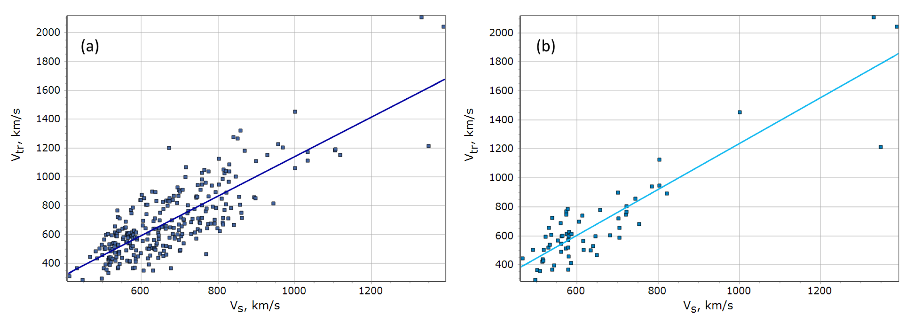
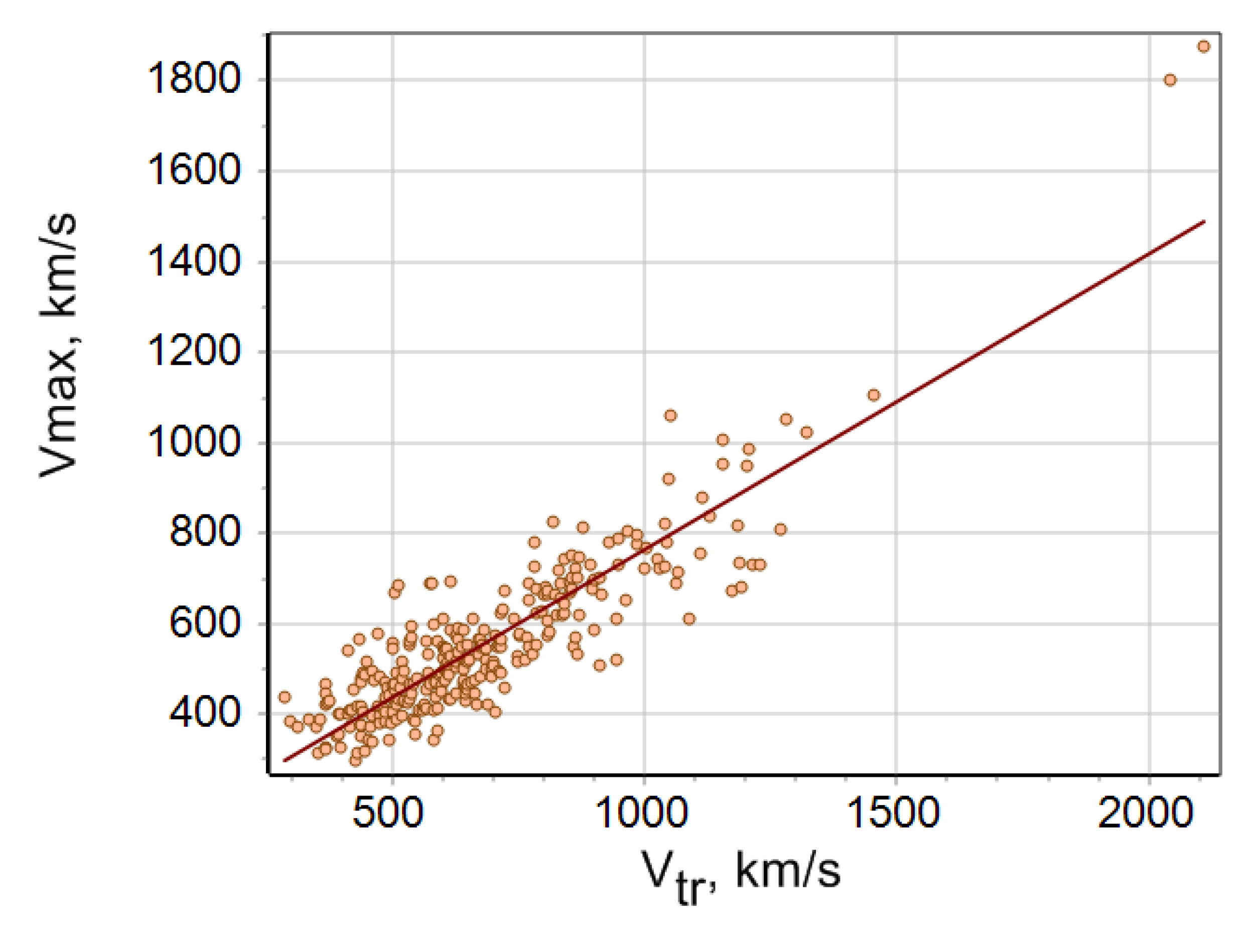
3.1. Relation between the ICME Transit Speed and the CME Initial Speed

It is well known that the initial CME speed ( V 0 ) largely determines the transit speed ( V t r ) of the corresponding ICME (the ratio of 1 AU to the propagation time of an ICME from the Sun to the Earth (see e.g., [34], and references therein). Figure 2 illustrates such a relation for the 288 events used in this study. It can be seen that there is a relationship ( c c = 0.64 ± 0.04), but with some scatter. This is due to the fact that all CMEs are different, i.e., some of them are strongly decelerated, while others are accelerated in the solar corona, and they may also interact with other ICMEs, high-speed streams (HSSs) from coronal holes (CHs), the heliospheric current sheet (HCS), etc. It is worth noting that the connection between the transit and initial CME speeds are not completely linear, as has been shown in [23,26]. Moreover, [53] showed that CMEs with similar initial velocities have the differences in their transit times up to several days. In our work, we want to check the linearity of the ICME transit speed on CME initial speed dependence and also examine whether a dependence on longitude exists.

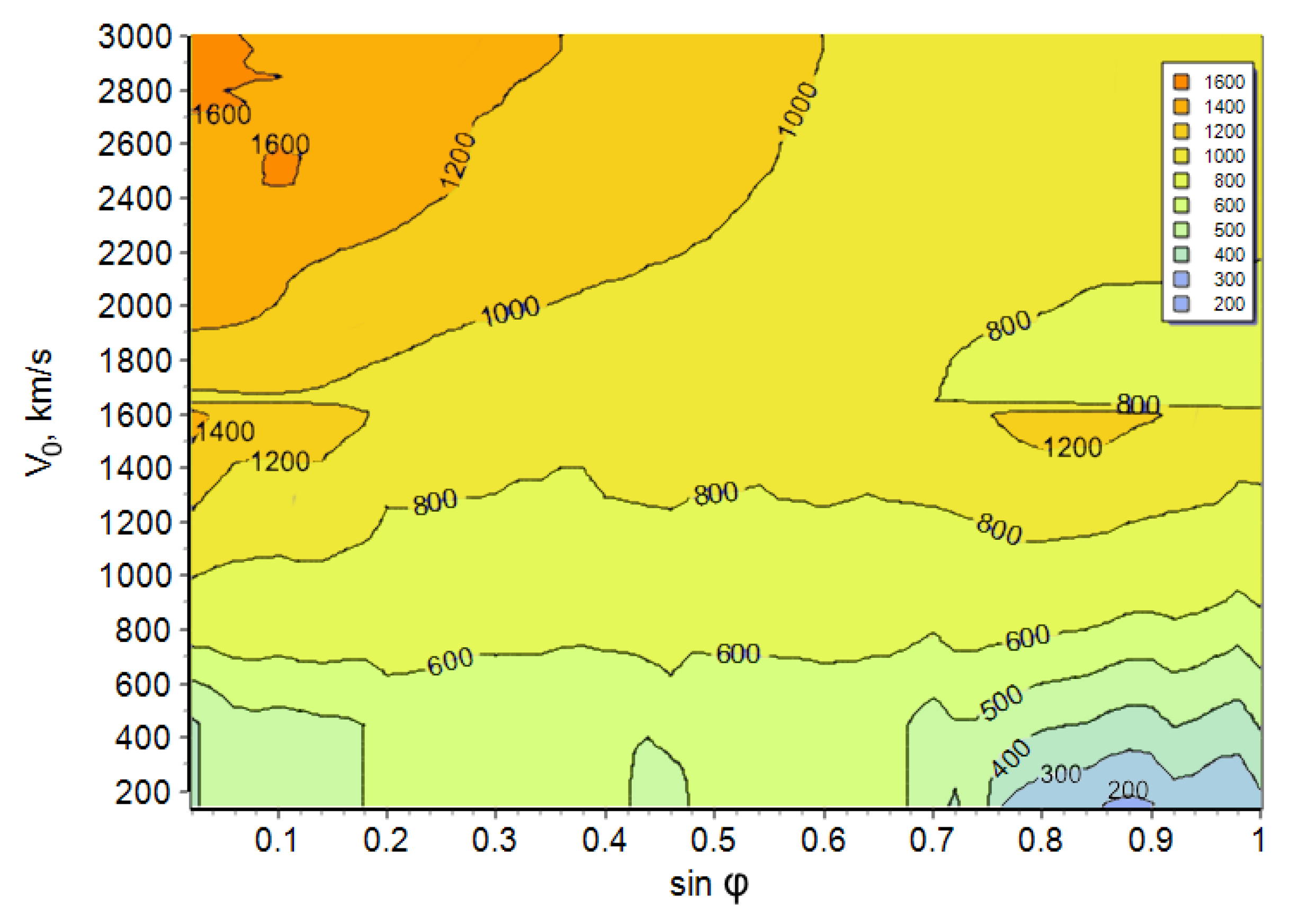
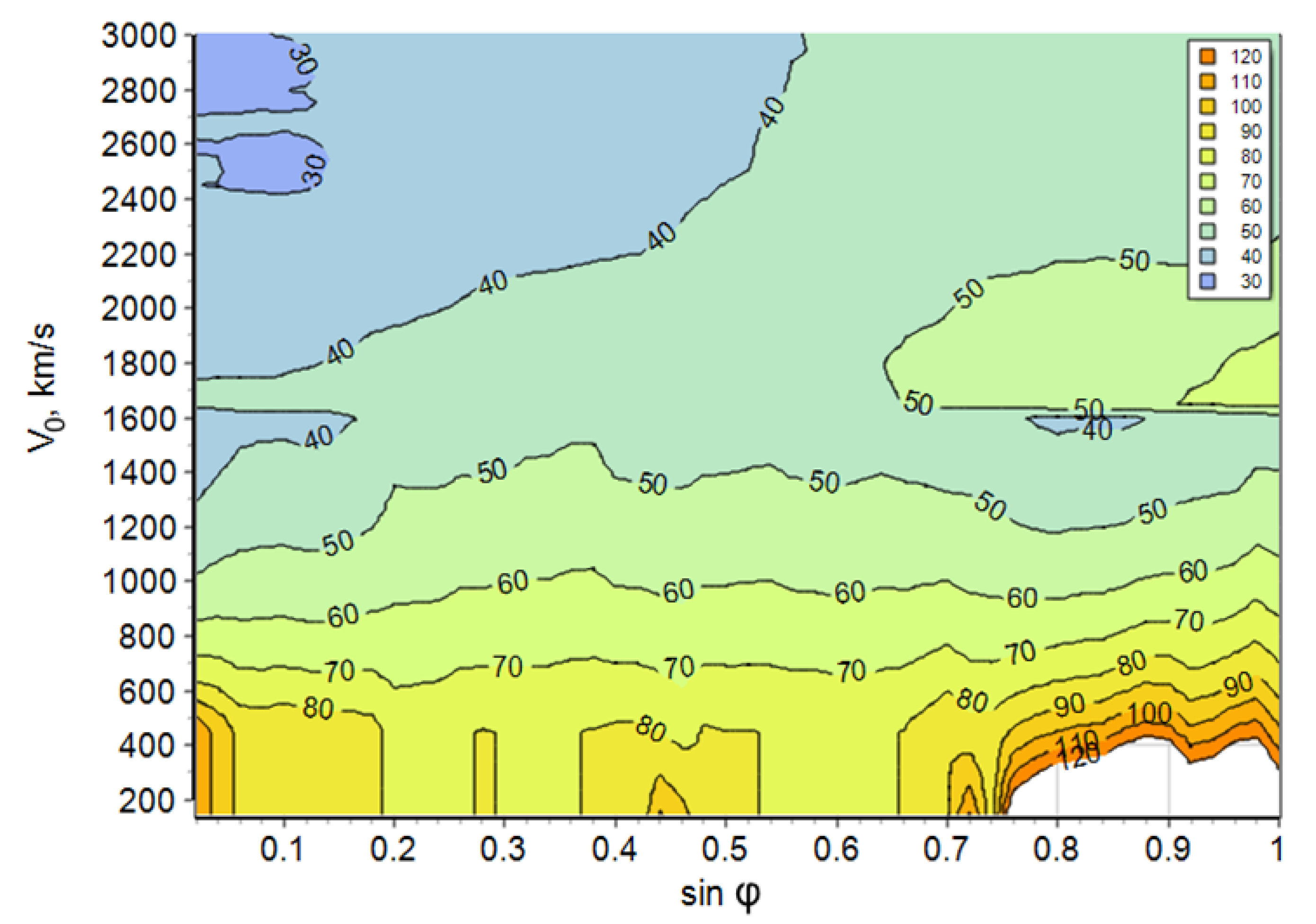
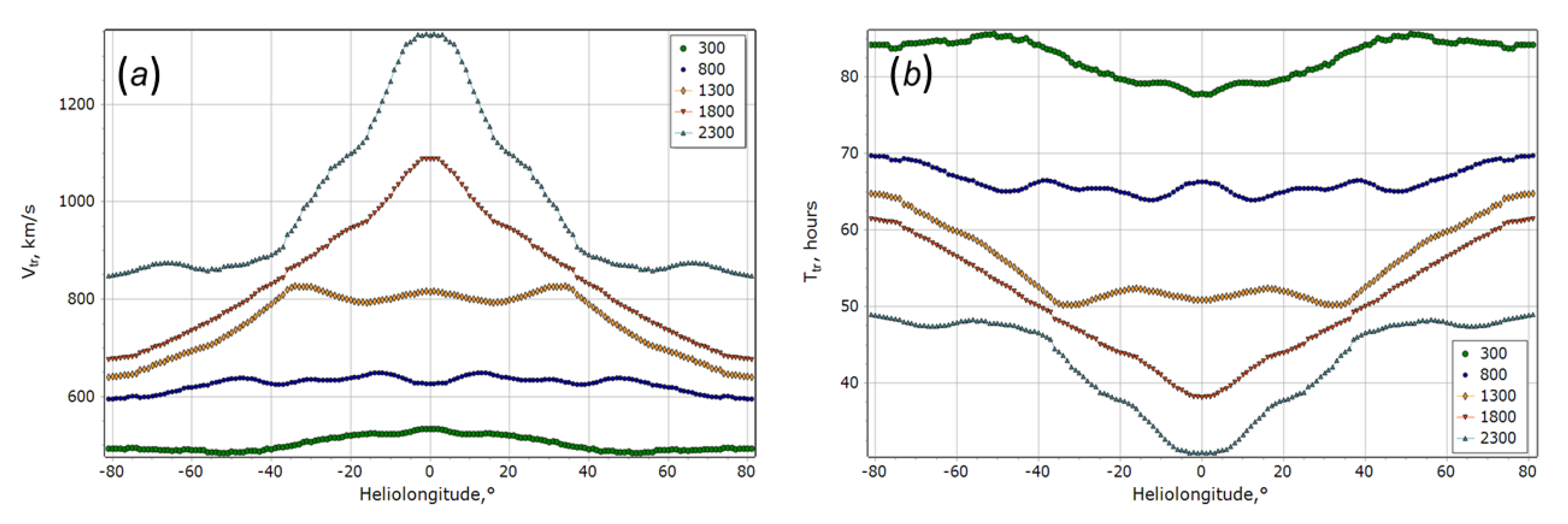
3.2. Speed’s Longitudinal Dependence

The non-linearity of the relationship between the initial and the transit CME/ICME speeds mentioned above is apparently explained by the fact that in the range of low velocities there exists both ICMEs that decelerate and slow down together with those that accelerate. On top of that, it has been shown that some very slow CMEs (with an initial speed of 150–200 km/s) are not distinguished according to the coronagraphic data, but could be recorded at Earth with a speed of 350–400 km/s [23,54]. Thus, for the central zone there is an artificial depletion in slow CMEs, since many of them fall into the “stealth” or problematic category (the CMEs that can be observed but there is no signature on the solar disk or are invisible for coronagraphs as they become very rarefied by the time they can be registered at the edge of the coronagraph screen but then hit the Earth, (see e.g., [20,55,56])).
The dependence of the transit speed of an ICME ( V t r ) on the initial speed of the corresponding CME ( V 0 ), taking into account the possible non-linearity for low-speed CMEs, can be represented as:
V t r = V c V 0 V c A + B V 0 V 0 > V c
where V c is the cut-off speed.
We plotted the dependences of V t r on V 0 for different ranges of absolute longitudes: ϕ 8 ° (Figure 3a) and 15 ° ϕ 24 ° (Figure 3b), the horizontal part of the graph in the figures reflects the non-linearity of the dependence. It is worth adding that we could try to choose a more complex dependence to describe this non-linear effect, but since it is observed in a very narrow range of velocities, the number of events that would allow a reliable identification is not adequate, and thus we decided to stop at the simplest dependence.
The correlation coefficient turned out to be c c = 0.91 ± 0.06 for 57 interplanetary disturbances in Figure 3a and c c = 0.81 ± 0.08 for 52 interplanetary disturbances in Figure 3b. Note that without taking into account the non-linear dependence the correlation coefficients were 0.88 ± 0.06 and 0.77 ± 0.09, respectively. Comparing the figures allows us to conclude that the dependence of the ICME transit speed on the initial CME speed changes with longitude: with an increase in the absolute value of longitude, the slope of the curve becomes much smaller, and the value of the regression coefficient (B) decreases from 0.8 ± 0.06 (Figure 3a) to 0.4 ± 0.06 (Figure 3b). It should be assumed that the non-linearity in the range of low velocities is significant only for central events. This is due to the fact that slow events simply “disappear" for large longitudes, since for them, the projection effects are much less pronounced.
We should also note that for central events, the speed threshold ( V c ) turns out to be artificially overestimated; the revealed non-linearity was expected for lower speed values, close to the quiet SW speed (400 km/s), but it turned out that it extends to a value of V c ∼ 520 km/s. This value of the cut-off speed was obtained from the data: different values were considered with a step of 10 km/s, and as a result, we settled on 520 km/s since the smallest dispersions were obtained at different longitude intervals for this cut-off speed value. A slightly better result could be obtained using average speeds, but we preferred a continuous relationship.
For large longitudes, the discussed non-linearity is not observed due to the fact that slow CMEs with a solar source far in longitude simply do not reach the Earth. Additionally, if we are talking about powerful events, it can be argued that the non-linearity will not be revealed, in particular for a sample of high-speed CMEs that created interplanetary shock waves observed near the Earth.
The analysis performed allows us to state that taking into account the heliolongitude of the solar source is important, as well as the non-linearity of the dependence of the transit ICME speed on the initial CME speed for central events, and they should be included in the parameters of the model being created.

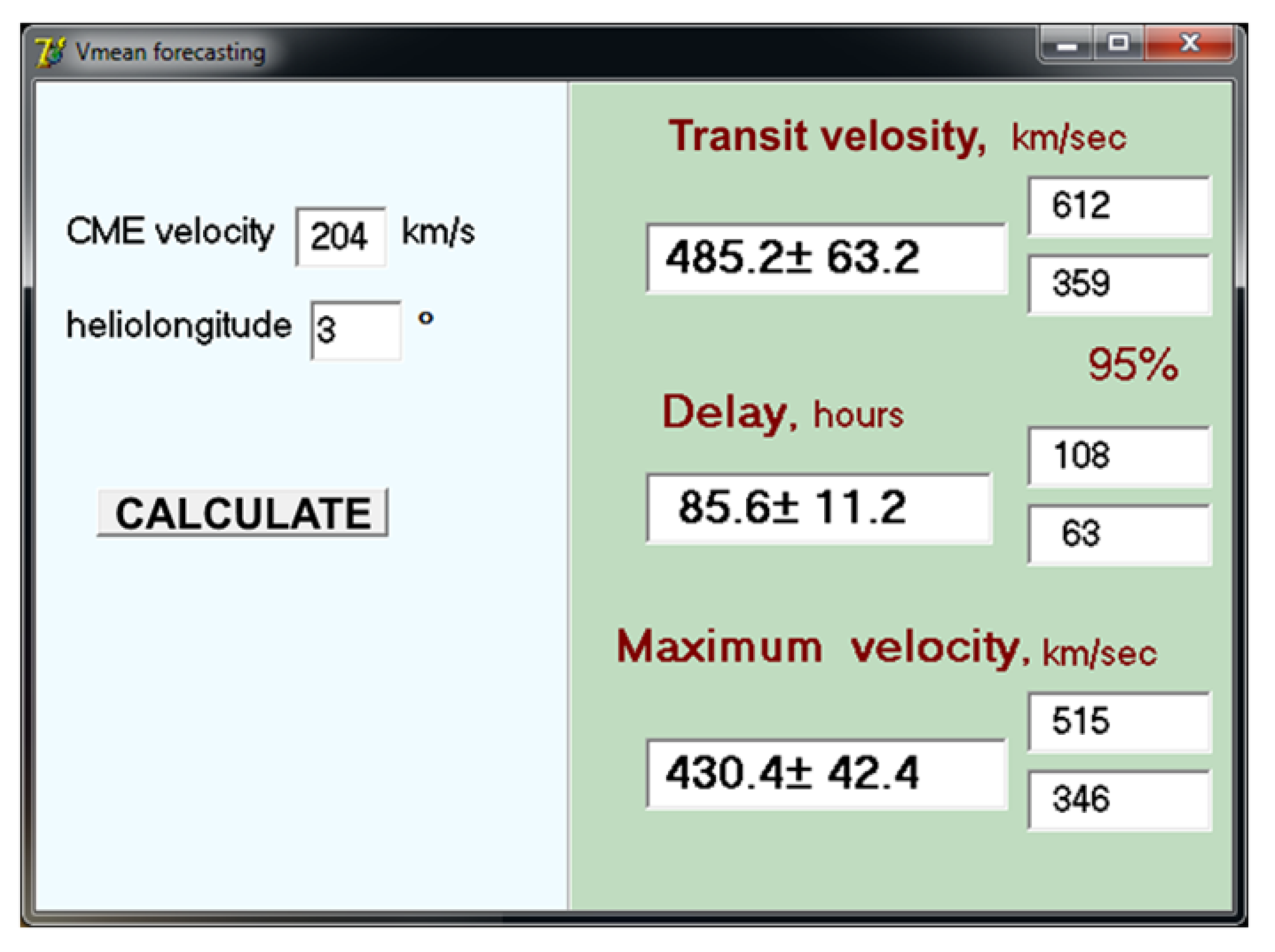
3.3. Model for Estimating the ICME Transit Speed and Time from Solar Data

Based on the data described above, we found that for a fairly wide central range, the cutoff speed remained unchanged at 520 km/s. For each interval of the sine of absolute heliolongitude (using a running window with a width of 0.14 and a step of 0.01, up to s i n ϕ = 0.9 inclusive, there were 64 of them in total, as for some intervals there were less than 10 events, these points were not used in the figure), a linear regression described above (see Equation (1)) was made and the average values of s i n ϕ for each interval were calculated, as well as regression and correlation coefficients. Their distribution depending on the sine of the absolute heliolongitude of the solar source is shown in Figure 4.
The regression coefficients A and B (Figure 4a) change in a complex way, and it should be assumed that this complexity is only to a small extent due to the fact that we use a limited sample and there are statistical fluctuations. Large-scale changes in these parameters (for example, a sharp increase in A values and a decrease in B values in the intervals of 0–12 ° (0 < s i n ϕ < 0.2) and 42 ° –60 ° (0.66 < s i n ϕ < 0.86) are apparently explained precisely by the peculiarities of the CME observation and the existence of projection effects (firstly, a statistically underestimated CME speed on the limbs, and secondly, a statistically overestimated speed in the central zone due to the lack of slow CMEs). It turns out that of these two effects, the maxima are observed for one in the center, and for the other—close to the limbs, they are superimposed on each other and when considering the distribution in longitude give the complexity observed in the figure. Moreover, these features are partly related to the shape of the ICMEs themselves, because they are not completely spherical, the sphericity is necessarily violated, for example, for the central part of ICME the speed is usually greater than at the edges.
As for the distribution of correlation coefficients (Figure 4b), the highest values are observed in the central region (up to ∼30 ° or sinϕ < 0.5), where most of the considered events are located, except for a small range of 12–18 ° (0.2 < s i n ϕ < 0.3) for which the statistics turned out to be less. It should be noted that the created model is also most useful for predicting the speed and time delay of interplanetary disturbances with a source in the central zone. For the middle range (30–50 ° or 0.5 < s i n ϕ < 0.76), the correlation coefficient decreases but still remains within the moderate relationship.
Our proposed model covers a wide range of longitudes from E60 ° to W60 ° , but outside this limit there are not enough events to establish a more reliable relation; however, we can still use the model for far events. In some rather rare events that originate from large solar longitudes, we cannot exactly assess whether the IP disturbance reaches the Earth. However, we can consider that the IP disturbance is less likely to be registered at Earth after the estimated ToA. In our sample, there are 12 events with absolute longitudes greater than 80 ° , and in most of them only the shock waves reached the Earth. Sometimes, such events produce magnetic storms, but more often their geoeffectiveness is low. It is also important for predicting the state of space weather environment.
Since it was shown above that the ICME transit time and speed depend not only on the initial speed of the parent CME but also on the longitude of the solar source, it is natural to expect that in some events the expected transit speed and time will be close to previously observed events with similar solar data: V 0 and s i n ϕ . This means that we can use the events that are already in our database, taking into account the identified links to determine the expected transit speed and time of a new event averaging the available information in the vicinity of the point under study. In this case, the contribution of neighboring points should also be taken into account so that the nearest points have the largest weight. The transit speed is calculated as follows:
V t r ( V 0 , s i n ϕ ) = i = 1 N V i w i i = 1 N w i
where V i is the speed of i-th event in the vicinity, w i —the weight of i-th event in the vicinity, N—the number of events in the vicinity. Wherein the weight of i-th event is defined as:
w i = 1 s v 2 + s p 2 + s o 2 s v s v c   a n d   | s p | 0.4 w i = 0 for any other values of s v and s p
where s v = | ( 1 V ) / V 0 i | , s p = ( s i n p s i n ϕ i ) , s i n p —the sine of absolute heliolongitude of the associated flare for event under study, V—the initial CME speed of the studied event, s i n ϕ i and V 0 i —the sine of absolute heliolongitude of associated flare and the initial speed of the i-th CME in the vicinity, s v c = 1 for V ≤ 300 km/s and s v c = 0.5 for V > 300 km/s, s 0 —a manually set value that defines the nearest vicinity where the weights barely change (default is s 0 = 0.1).
The number of points actually participating in the determination of V t r will be different but N = 288 taking into account expression (3).
The values of speed errors are calculated in the same way as the speeds themselves (taking into account the weight) but instead of the speed value, the difference between the predicted and observed transit velocities (in absolute value) is taken. For nodes evenly spaced in speed (with a step of 50 km/s) and s i n ϕ (with a step of 0.02) the matrices of expected values of transit speed and time and their statistical errors were calculated. To do this, in each node, the values of transit speed were calculated according to Formula (2) and ToA according to Formula (4):
T t r = 1 A U V t r
Based on the calculated data matrices, we also obtained a contour representation (Figure 5 and Figure 6) of the expected values of the transit speed and the ToA of an ICME at Earth depending on the initial CME speed and the heliolongitude of the source (associated solar flare). Using these figures and the data on the initial CME speed and heliolongitude of associated flare, one can estimate the interval of the expected transit speed and time of the corresponding ICME (numbers indicated on the corresponding isolines).
The highest velocities are expected for the central events, while relatively low velocities are observed over the entire range of longitudes. In general, it can be concluded that in order to obtain the same transit speeds when comparing events with different heliolongitudes, large initial CME velocities for large longitudes are required (applicable to the studied sample of events). For example, for an ICME transit speed of 800 km/s, the parent CME in the central zone (up to 20 ° ) should have an initial speed of 1000–1100 km/s, and if the parent CME is closer to the limb (>70 ° ), then its initial speed should already be 1200–1400 km/s. Or, conversely, if the initial CME speed is 1500 km/s, then in the case of a central source the transit speed is expected to be about 1300 km/s, and in the case of a limb source it is much less, about 800 km/s.
Similar reasoning is applicable to the comparison of an ICME ToA (see Figure 6). The fastest ICMEs are recorded on Earth within about 30 h after solar flares (blue range), and the slowest are more than 90 h (orange range). Although there are some unique events (for example, October, 2003) for which the transit time turned out to be less than 20 h, there are very few of them, so one cannot speak of statistically significant results of their assessment.
Let us give examples of using the isolines of the expected ICME transit time according to Figure 6. For a CME with an initial speed of 1000 km/s with a source in the central zone, the expected arrival time is about 50 h; for a similar CME with a limb source, it is 60–70 h. Moreover, to wait for the Earth impact of an ICME, for example, within 30 hours after the associated flare, the parent CME in the central zone should have an initial speed above 2400 km/s; as for the limb events, there are no similar arrival times recorded earlier.
We also obtained dependences of expected transit velocities ( V t r ) and ToA ( T t r ) on the longitude of the corresponding flare. From Figure 7a,b (as well as using contours) it is possible to determine what the expected transit speed will be depending on the longitude of the CME source and its initial speed.
The features are explained by two factors that we have already mentioned. First, the projection effect that leads, in particular, to artificial depletion by low-speed CMEs in the central zone. This is because they often cannot be registered by coronagraphs and the CME speed towards the Earth for central events is usually higher than in the picture plane. Second, for events that emerge from the near limb zone, there is an overestimation of the ICME transit speed and an underestimation of the transit time, because for such ICMEs, their lower-speed flank, rather than the nose part, hits the Earth.
Using data matrices mentioned above, we have the ability to calculate the expected ICME speed for any longitude and initial CME speed, in particular, for those points that served as the main sample for the analysis. Figure 8a,b shows plots of the observed speed in the events under study ( V t r ) and the speed calculated by the model ( V S ) for (a) all events in the sample and for (b) events in the central part of solar disk with longitudes ϕ < 10 ° . The correlation coefficient for the entire sample (288 events) is c c = 0.8 ± 0.035, and for the central events (63 events) is c c = 0.9 ± 0.055. Recall that the initial similar distribution had c c = 0.64 ± 0.04 (see Figure 2), so we can assume that we have significantly improved the result. It can be seen that in Figure 8 the scatter of points is quite large (about ±200 km/s), and there is still a prospect for improvement.
The average absolute deviation of ToA for the created model is 11.6 h (for 288 events). Note that the average absolute deviation of ToA for the initial empirical relationship without taking into account solar sources longitudes (see Figure 2) was 13.4 h.
The created model makes it possible to estimate not only the transit speed of ICMEs, but also the maximum speed of such interplanetary disturbances near Earth (the maximum speed of the ejecta in the period of the ICME passage observed in situ by spacecrafts).The estimate of the maximum speed recorded in an event is based on the regression presented in Figure 9. It has been established that the maximum speed in the events of the studied sample correlates very well with their actual transit speed ( c c = 0.89 ± 0.027), so the estimates can be considered reliable. This is important, since the estimate of the maximum speed in an event is significant for more accurate prediction of the space weather state and disturbances power in the Earth’s magnetosphere.
The developed model is already being used in the daily practice of the IZMIRAN Space Weather Prediction Center (http://spaceweather.izmiran.ru/eng/index.html). Figure 10 shows a screenshot of the working version of the program used to calculate the transit and maximum speeds of an ICME, as well as the time of its arrival to Earth, which is based on the model described here above.
The numbers shown in the figure correspond to the calculation performed for the event of 13 May 2021 associated with the B1.3 flare at 18:07 UT which occurred in AR12822 (N18W03), and the subsequent eruption of the solar filament recorded in the coronagraph data at 19:36 UT with the initial speed of 204 km/s. According to our calculations, the corresponding ICME should have reached the Earth’s orbit on 17 May 2021 at 08:12 UT ± 11.2 h, and the shock arrival according to the DISCOVR satellite data occurred on 17 May 2021 at 15:46 UT, i.e., our estimation was satisfactory. Note that according to the ISWA model (https://iswa.gsfc.nasa.gov/IswaSystemWebApp/), the arrival of this ICME into the Earth’s orbit was predicted earlier: on 16 May 2021 at 21:49 ± 7 h.
Our estimation of the maximum speed (430.4 ± 42.4 km/s) for this event turned out to be somewhat overstated in comparison with the actually observed maximum values of the SW speed (370 km/s for the second half of 17 May 2021 according to OMNI, https://omniweb.gsfc.nasa.gov/). The delay in the time of registration and the decrease in the speed of this ICME can be explained by the fact that the Earth was in another SW disturbance in the previous day. In the given example, the estimate of the transit speed turned out to be satisfactory. However, it should be taken into account that, in the studied sample, only 22.2% of events had an initial CME speed < 400 km/s, so our model is more adapted to estimating CMEs of higher speeds. We also tried to find as an example a fast and powerful event. However, at the moment in the used CME catalog (https://cdaw.gsfc.nasa.gov/CME_list/) for the year of 2021, there are no events that could belong to the control group (fast central CMEs that reached the Earth). A series of flares and subsequent CMEs suitable for these conditions registered in May 2021 turned out to be difficult to separate from each other, so the calculations for them have been considered unreliable.

4. Conclusions

We have reviewed and analyzed 288 CMEs registered with the SOHO/LASCO coronagraph, associated with solar flares and then observed in near-Earth space.
It is shown that the relationship between an ICME transit speed and the initial CME speed is non-linear at low velocities, which confirms the results reported in previous works (e.g., [23,24]). The revealed non-linearity is most pronounced for CMEs from the central heliolongitudinal zone.
It has been established that ICMEs transit speed and time of arrival (ToA) depend not only on the initial speed of the corresponding CME but also on the longitude of the associated solar flare.
It is shown that the ICME transit speed in the studied sample of 288 events is closely related to the maximum speed observed on Earth.
A model has been created that takes into account the solar data that accompany the generation of CMEs: initial speed and heliolongitude of the source, which makes it possible to estimate ICMEs transit speed and arrival time, as well as the maximum speed of the interplanetary disturbance in near-Earth space. Accounting for the longitude of solar sources significantly improves the quality of the model.
The results obtained are applicable in forecasting a state of space weather.
In the future it is planned to expand the statistics used in the model and carry out work to improve the quality of estimates. Low-speed CMEs should be investigated separately. Perhaps it is worth considering more carefully the events at different phases of the solar cycle, since, for example, ref. [57] showed that at different phases of the solar cycle there is a different CME deflection resulting from the background solar magnetic field. It is also planned to combine the created model with the model of the ICMEs arrival probability which will improve our estimates for events with large longitudes of solar sources. Recall that all the results obtained do not apply to all CMEs, but only to those that were reliably identified in coronagraphic data and the corresponding ICMEs reached the Earth. Nevertheless, a wider application of our model is also possible, for example, for solving the inverse problem: estimating the initial CME velocities from the observed transit times, in cases where the coronagraphic data were absent or unreliable. In addition, in this paper, we considered those events for which the initial, transit, and maximum speeds were known, but there are a lot of events for which we know only the transit speed (19th solar cycle events, for example), and the relationships we identified can be used to estimate the CME speed and the maximum SW disturbance speed. This is also a task for future research.

Author Contributions

Conceptualization, A.B. and M.A.; methodology, N.S.; software, A.A.; analysis, M.A., N.S., A.B. and A.P.; data curation, A.A. and A.P.; writing—original draft preparation, N.S.; writing—review and editing, A.P., M.A. and A.B. All authors have read and agreed to the published version of the manuscript.

Funding

A.A., M.A., A.B. and N.S. are supported by the Russian Science Foundation grant No. 20–72-10023.

Data Availability Statement

The study made use of the CDAW CME catalogue; https://cdaw.gsfc.nasa.gov/CME_list/. The Forbush Effects and Interplanetary Disturbances Database (FEID, http://spaceweather.izmiran.ru/eng/dbs.html). FEID incorporates SW and IMF parameters taken from the OMNI database (https://omniweb.gsfc.nasa.gov/), the list of shock waves—http://isgi.unistra.fr/data_download.php, and the catalogue of flares—https://www.ngdc.noaa.gov/stp/space-weather/solar-data/solar-features/solar-flares/x-rays/goes/xrs/.The study further makes use of daily movies from SOHO (https://soho.nascom.nasa.gov/data/realtime/mpeg/), SDO (https://sdo.gsfc.nasa.gov/data/dailymov.php) and STEREO (https://stereo-ssc.nascom.nasa.gov/beacon/beacon_secchi.shtml); ICME catalogues (e.g., https://izw1.caltech.edu/ACE/ASC/DATA/level3/icmetable2.htm, http://www.iki.rssi.ru/omni/catalog/), as well as other sources of solar data (for example, solarmonitor.org) and models (for example, https://iswa.gsfc.nasa.gov/IswaSystemWebApp/, https://www.swpc.noaa.gov/products/wsa-enlil-solar-wind-prediction.

Acknowledgments

This CME catalog is generated and maintained at the CDAW Data Center by NASA and The Catholic University of America in cooperation with the Naval Research Laboratory. SOHO is a project of international cooperation between ESA and NASA.

Conflicts of Interest

The authors declare no conflict of interest.

References

  1. Gosling, J.T.; Bame, S.J.; McComas, D.J.; Phillips, J.L. Coronal mass ejections and large geomagnetic storms. Geophys. Res. Lett. 1990, 17, 901–904. [Google Scholar] [CrossRef]
  2. Tsurutani, B.T.; Gonzalez, W.D. The Interplanetary causes of magnetic storms: A review. Wash. DC Am. Geophys. Union Geophys. Monogr. Ser. 1997, 98, 77–89. [Google Scholar] [CrossRef]
  3. Zhang, J.; Dere, K.P.; Howard, R.A.; Bothmer, V. Identification of Solar Sources of Major Geomagnetic Storms between 1996 and 2000. Astrophys. J. 2003, 582, 520–533. [Google Scholar] [CrossRef]
  4. Webb, D.F.; Howard, T.A. Coronal Mass Ejections: Observations. Living Rev. Sol. Phys. 2012, 9, 3. [Google Scholar] [CrossRef]
  5. Zhang, J.; Temmer, M.; Gopalswamy, N.; Malandraki, O.; Nitta, N.V.; Patsourakos, S.; Shen, F.; Vršnak, B.; Wang, Y.; Webb, D.; et al. Earth-affecting solar transients: A review of progresses in solar cycle 24. Prog. Earth Planet. Sci. 2021, 8, 56. [Google Scholar] [CrossRef]
  6. Michałek, G.; Gopalswamy, N.; Yashiro, S. A New Method for Estimating Widths, Velocities, and Source Location of Halo Coronal Mass Ejections. Astrophys. J. 2003, 584, 472–478. [Google Scholar] [CrossRef]
  7. Wang, Y.; Shen, C.; Wang, S.; Ye, P. Deflection of coronal mass ejection in the interplanetary medium. Sol. Phys. 2004, 222, 329–343. [Google Scholar] [CrossRef]
  8. Gopalswamy, N. Consequences of Coronal Mass Ejections in the Heliosphere. Sun Geosph. 2006, 1, 5–12. [Google Scholar]
  9. Gopalswamy, N.; Yashiro, S.; Akiyama, S.; Mäkelä, P.; Xie, H.; Kaiser, M.L.; Howard, R.A.; Bougeret, J.L. Coronal mass ejections, type II radio bursts, and solar energetic particle events in the SOHO era. Ann. Geophys. 2008, 26, 3033–3047. [Google Scholar] [CrossRef]
  10. Richardson, I.G.; Cane, H.V. Near-Earth Interplanetary Coronal Mass Ejections During Solar Cycle 23 (1996–2009): Catalog and Summary of Properties. Sol. Phys. 2010, 264, 189–237. [Google Scholar] [CrossRef]
  11. Wu, C.C.; Lepping, R.P. Relationships Among Geomagnetic Storms, Interplanetary Shocks, Magnetic Clouds, and Sunspot Number During 1995–2012. Sol. Phys. 2016, 291, 265–284. [Google Scholar] [CrossRef]
  12. Chi, Y.; Shen, C.; Wang, Y.; Xu, M.; Ye, P.; Wang, S. Statistical Study of the Interplanetary Coronal Mass Ejections from 1995 to 2015. Sol. Phys. 2016, 291, 2419–2439. [Google Scholar] [CrossRef]
  13. Hess, P.; Zhang, J. A Study of the Earth-Affecting CMEs of Solar Cycle 24. Sol. Phys. 2017, 292, 80. [Google Scholar] [CrossRef]
  14. Hildner, E.; Gosling, J.T.; MacQueen, R.M.; Munro, R.H.; Poland, A.I.; Ross, C.L. Frequency of coronal transients and solar activity. Sol. Phys. 1976, 48, 127–135. [Google Scholar] [CrossRef]
  15. Gosling, J.T.; Hildner, E.; MacQueen, R.M.; Munro, R.H.; Poland, A.I.; Ross, C.L. The speeds of coronal mass ejection events. Sol. Phys. 1976, 48, 389–397. [Google Scholar] [CrossRef]
  16. Hundhausen, A.J.; Burkepile, J.T.; St. Cyr, O.C. Speeds of coronal mass ejections: SMM observations from 1980 and 1984–1989. J. Geophys. Res. Space Phys. 1994, 99, 6543–6552. [Google Scholar] [CrossRef]
  17. Lindsay, G.M.; Luhmann, J.G.; Russell, C.T.; Gosling, J.T. Relationships between coronal mass ejection speeds from coronagraph images and interplanetary characteristics of associated interplanetary coronal mass ejections. J. Geophys. Res. Space Phys. 1999, 104, 12515–12524. [Google Scholar] [CrossRef]
  18. Yashiro, S.; Gopalswamy, N.; Akiyama, S.; Michalek, G.; Howard, R.A. Visibility of coronal mass ejections as a function of flare location and intensity. J. Geophys. Res. Space Phys. 2005, 110, A12S05. [Google Scholar] [CrossRef]
  19. Wang, Y.; Chen, C.; Gui, B.; Shen, C.; Ye, P.; Wang, S. Statistical study of coronal mass ejection source locations: Understanding CMEs viewed in coronagraphs. J. Geophys. Res. Space Phys. 2011, 116, A04104. [Google Scholar] [CrossRef]
  20. Chi, Y.; Zhang, J.; Shen, C.; Hess, P.; Liu, L.; Mishra, W.; Wang, Y. Observational Study of an Earth-affecting Problematic ICME from STEREO. Astrophys. J. 2018, 863, 108. [Google Scholar] [CrossRef]
  21. Cane, H.V.; Richardson, I.G.; St. Cyr, O.C. Coronal mass ejections, interplanetary ejecta and geomagnetic storms. Geophys. Res. Lett. 2000, 27, 3591–3594. [Google Scholar] [CrossRef]
  22. Wang, Y.M.; Ye, P.Z.; Wang, S.; Zhou, G.P.; Wang, J.X. A statistical study on the geoeffectiveness of Earth-directed coronal mass ejections from March 1997 to December 2000. J. Geophys. Res. Space Phys. 2002, 107, 1340. [Google Scholar] [CrossRef]
  23. Gopalswamy, N.; Lara, A.; Lepping, R.P.; Kaiser, M.L.; Berdichevsky, D.; St. Cyr, O.C. Interplanetary acceleration of coronal mass ejections. Geophys. Res. Lett. 2000, 27, 145–148. [Google Scholar] [CrossRef]
  24. Gopalswamy, N.; Lara, A.; Yashiro, S.; Kaiser, M.L.; Howard, R.A. Predicting the 1-AU arrival times of coronal mass ejections. J. Geophys. Res. Space Phys. 2001, 106, 29207–29218. [Google Scholar] [CrossRef]
  25. Vršnak, B.; Žic, T. Transit times of interplanetary coronal mass ejections and the solar wind speed. Astron. Astrophys. 2007, 472, 937–943. [Google Scholar] [CrossRef]
  26. Vršnak, B.; Sudar, D.; Ruždjak, D.; Žic, T. Projection effects in coronal mass ejections. Astron. Astrophys. 2007, 469, 339–346. [Google Scholar] [CrossRef]
  27. Temmer, M.; Preiss, S.; Veronig, A.M. CME Projection Effects Studied with STEREO/COR and SOHO/LASCO. Sol. Phys. 2009, 256, 183–199. [Google Scholar] [CrossRef]
  28. Bronarska, K.; Michalek, G. Determination of projection effects of CMEs using quadrature observations with the two STEREO spacecraft. Adv. Space Res. 2018, 62, 408–416. [Google Scholar] [CrossRef]
  29. Paouris, E.; Vourlidas, A.; Papaioannou, A.; Anastasiadis, A. Assessing the Projection Correction of Coronal Mass Ejection Speeds on Time of Arrival Prediction Performance Using the Effective Acceleration Model. Space Weather 2021, 19, e02617. [Google Scholar] [CrossRef]
  30. Lara, A.; Gopalswamy, N.; Xie, H.; Gonzalez-Esparza, A. Sun-Earth Propagation Time of CMEs Originated at different Helio Longitudes. Eos Trans. AGU 2005, 86, SH53A-10. [Google Scholar]
  31. Anna Lakshmi, M.; Umapathy, S.; Prakash, O.; Vasanth, V. Studies on some properties of coronal mass ejections based on angular width. Astrophys. Space Sci. 2011, 335, 373–378. [Google Scholar] [CrossRef]
  32. Nedal, M.; Youssef, M.; Mahrous, A.; Helal, R. Investigating the Coronal Mass Ejections associated with DH type-II radio bursts and solar flares during the ascending phase of the solar cycle 24. Adv. Space Res. 2019, 63, 1824–1836. [Google Scholar] [CrossRef]
  33. Vršnak, B.; Gopalswamy, N. Influence of the aerodynamic drag on the motion of interplanetary ejecta. J. Geophys. Res. Space Phys. 2002, 107, 1019. [Google Scholar] [CrossRef]
  34. Shanmugaraju, A.; Vršnak, B. Transit Time of Coronal Mass Ejections under Different Ambient Solar Wind Conditions. Sol. Phys. 2014, 289, 339–349. [Google Scholar] [CrossRef]
  35. Odstrcil, D. Modeling 3-D solar wind structure. Adv. Space Res. 2003, 32, 497–506. [Google Scholar] [CrossRef]
  36. Tóth, G.; Sokolov, I.V.; Gombosi, T.I.; Chesney, D.R.; Clauer, C.R.; de Zeeuw, D.L.; Hansen, K.C.; Kane, K.J.; Manchester, W.B.; Oehmke, R.C.; et al. Space Weather Modeling Framework: A new tool for the space science community. J. Geophys. Res. Space Phys. 2005, 110, A12226. [Google Scholar] [CrossRef]
  37. McKenna-Lawlor, S.M.P.; Dryer, M.; Kartalev, M.D.; Smith, Z.; Fry, C.D.; Sun, W.; Deehr, C.S.; Kecskemety, K.; Kudela, K. Near real-time predictions of the arrival at Earth of flare-related shocks during Solar Cycle 23. J. Geophys. Res. Space Phys. 2006, 111, A11103. [Google Scholar] [CrossRef]
  38. Feng, X.; Zhou, Y.; Wu, S.T. A Novel Numerical Implementation for Solar Wind Modeling by the Modified Conservation Element/Solution Element Method. Astrophys. J. 2007, 655, 1110–1126. [Google Scholar] [CrossRef]
  39. Feng, X.; Yang, L.; Xiang, C.; Wu, S.T.; Zhou, Y.; Zhong, D. Three-dimensional Solar WIND Modeling from the Sun to Earth by a SIP-CESE MHD Model with a Six-component Grid. Astrophys. J. 2010, 723, 300–319. [Google Scholar] [CrossRef]
  40. Shen, F.; Feng, X.; Wu, S.T.; Xiang, C. Three-dimensional MHD simulation of CMEs in three-dimensional background solar wind with the self-consistent structure on the source surface as input: Numerical simulation of the January 1997 Sun-Earth connection event. J. Geophys. Res. Space Phys. 2007, 112, A06109. [Google Scholar] [CrossRef]
  41. Davies, J.A.; Harrison, R.A.; Perry, C.H.; Möstl, C.; Lugaz, N.; Rollett, T.; Davis, C.J.; Crothers, S.R.; Temmer, M.; Eyles, C.J.; et al. A Self-similar Expansion Model for Use in Solar Wind Transient Propagation Studies. Astrophys. J. 2012, 750, 23. [Google Scholar] [CrossRef]
  42. Möstl, C.; Davies, J.A. Speeds and Arrival Times of Solar Transients Approximated by Self-similar Expanding Circular Fronts. Sol. Phys. 2013, 285, 411–423. [Google Scholar] [CrossRef]
  43. Núñez, M.; Nieves-Chinchilla, T.; Pulkkinen, A. Prediction of shock arrival times from CME and flare data. Space Weather 2016, 14, 544–562. [Google Scholar] [CrossRef]
  44. Paouris, E.; Mavromichalaki, H. Effective Acceleration Model for the Arrival Time of Interplanetary Shocks driven by Coronal Mass Ejections. Sol. Phys. 2017, 292, 180. [Google Scholar] [CrossRef]
  45. Dumbović, M.; Čalogović, J.; Vršnak, B.; Temmer, M.; Mays, M.L.; Veronig, A.; Piantschitsch, I. The Drag-based Ensemble Model (DBEM) for Coronal Mass Ejection Propagation. Astrophys. J. 2018, 854, 180. [Google Scholar] [CrossRef]
  46. Čalogović, J.; Dumbović, M.; Sudar, D.; Vršnak, B.; Martinić, K.; Temmer, M.; Veronig, A.M. Probabilistic Drag-Based Ensemble Model (DBEM) Evaluation for Heliospheric Propagation of CMEs. Sol. Phys. 2021, 296, 114. [Google Scholar] [CrossRef]
  47. Riley, P.; Mays, M.L.; Andries, J.; Amerstorfer, T.; Biesecker, D.; Delouille, V.; Dumbović, M.; Feng, X.; Henley, E.; Linker, J.A.; et al. Forecasting the Arrival Time of Coronal Mass Ejections: Analysis of the CCMC CME Scoreboard. Space Weather 2018, 16, 1245–1260. [Google Scholar] [CrossRef]
  48. Wold, A.M.; Mays, M.L.; Taktakishvili, A.; Jian, L.K.; Odstrcil, D.; MacNeice, P. Verification of real-time WSA-ENLIL+Cone simulations of CME arrival-time at the CCMC from 2010 to 2016. J. Space Weather Space Clim. 2018, 8, A17. [Google Scholar] [CrossRef]
  49. Iwai, K.; Shiota, D.; Tokumaru, M.; Fujiki, K.; Den, M.; Kubo, Y. Validation of coronal mass ejection arrival-time forecasts by magnetohydrodynamic simulations based on interplanetary scintillation observations. Earth Planets Space 2021, 73, 9. [Google Scholar] [CrossRef]
  50. Suresh, K.; Gopalswamy, N.; Shanmugaraju, A. Arrival Time Estimates of Earth-Directed CME-Driven Shocks. Sol. Phys. 2022, 297, 3. [Google Scholar] [CrossRef]
  51. Melkumyan, A.A.; Belov, A.V.; Abunina, M.A.; Abunin, A.A.; Eroshenko, E.A.; Oleneva, V.A.; Yanke, V.G. Main Properties of Forbush Effects Related to High-Speed Streams from Coronal Holes. Geomagn. Aeron. 2018, 58, 154–168. [Google Scholar] [CrossRef]
  52. Melkumyan, A.A.; Belov, A.V.; Abunina, M.A.; Abunin, A.A.; Eroshenko, E.A.; Yanke, V.G.; Oleneva, V.A. Comparison between statistical properties of Forbush decreases caused by solar wind disturbances from coronal mass ejections and coronal holes. Adv. Space Res. 2019, 63, 1100–1109. [Google Scholar] [CrossRef]
  53. Shen, C.; Wang, Y.; Pan, Z.; Miao, B.; Ye, P.; Wang, S. Full-halo coronal mass ejections: Arrival at the Earth. J. Geophys. Res. Space Phys. 2014, 119, 5107–5116. [Google Scholar] [CrossRef]
  54. Belov, A.; Abunin, A.; Abunina, M.; Eroshenko, E.; Oleneva, V.; Yanke, V.; Papaioannou, A.; Mavromichalaki, H.; Gopalswamy, N.; Yashiro, S. Coronal Mass Ejections and Non-recurrent Forbush Decreases. Sol. Phys. 2014, 289, 3949–3960. [Google Scholar] [CrossRef]
  55. Webb, D.F.; Cliver, E.W.; Gopalswamy, N.; Hudson, H.S.; St. Cyr, O.C. The solar origin of the January 1997 coronal mass ejection, magnetic cloud and geomagnetic storm. Geophys. Res. Lett. 1998, 25, 2469–2472. [Google Scholar] [CrossRef]
  56. Robbrecht, E.; Patsourakos, S.; Vourlidas, A. No Trace Left Behind: STEREO Observation of a Coronal Mass Ejection Without Low Coronal Signatures. Astrophys. J. 2009, 701, 283–291. [Google Scholar] [CrossRef]
  57. Kay, C.; Opher, M.; Evans, R.M. Global Trends of CME Deflections Based on CME and Solar Parameters. Astrophys. J. 2015, 805, 168. [Google Scholar] [CrossRef]
Figure 1. Distribution of the initial CME linear speeds depending on s i n ϕ for 288 events.
Universe 08 00327 g001
Figure 2. The relation of the initial CME speed ( V 0 ) and the transit speed of the corresponding ICME ( V t r ) for 288 events.
Universe 08 00327 g002
Figure 3. Dependence of the ICME transit speed on the parent CME initial speed for events with absolute heliolongitude: (a) ϕ 8 ° ; (b) 15 ° ϕ 24 ° .
Universe 08 00327 g003
Figure 4. Distribution of the regression coefficients (a) and the correlation coefficients (b) depending on s i n ϕ .
Universe 08 00327 g004
Figure 5. The relation of the expected ICME transit speed to the initial CME speed and the sine of the associated flare absolute heliolongitude. Different colors indicate the gradation of the expected transit speed in magnitude.
Universe 08 00327 g005
Figure 6. The relation of the expected ICME transit time to the initial CME speed and the sine of the associated flare absolute heliolongitude. Different colors indicate the gradation of the expected propagation time in magnitude.
Universe 08 00327 g006
Figure 7. Dependencies of the expected transit velocities [ V t r ] (a) and time of arrival ToA [ T t r ] (b) on the initial CME speed and longitude of the associated flare.
Universe 08 00327 g007
Figure 8. The relationship between actually observed and model-calculated ICME transit velocities for (a) the full sample; for (b) central events ϕ < 10 ° .
Universe 08 00327 g008
Figure 9. The relationship between the maximum and transit ICME speeds for 288 events under study.
Universe 08 00327 g009
Figure 10. Screenshot of the program for calculating the expected transit and maximum speed and propagation time of ICMEs created on the basis of the described model.
Universe 08 00327 g010
Publisher’s Note: MDPI stays neutral with regard to jurisdictional claims in published maps and institutional affiliations.

