
Constraints on the Helium Abundance from Fast Radio Bursts

Abstract
:1. Introduction
2. Properties of FRBs
3. Constraints from Current Data
4. Future Prospects
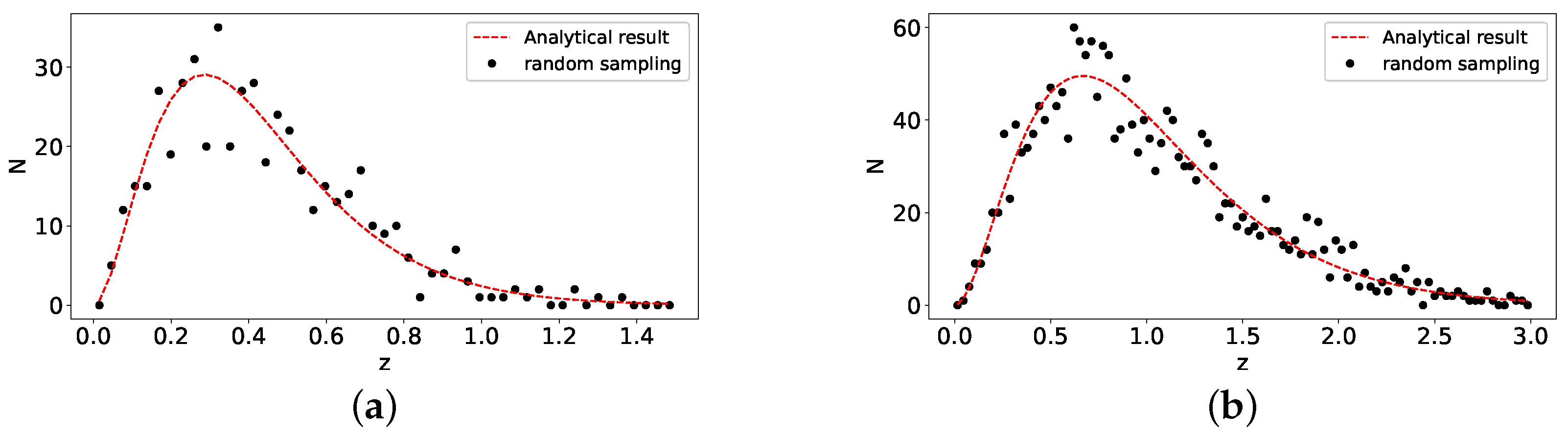
4.1. Mock Data
4.2. Shift Parameters
4.3. Results from DM and Shift Parameters
5. Conclusions
- Since the 17 current FRB samples have low redshift, resulting in poor quality of the samples, we could not obtain a useful constraint on the helium abundance, which is associated with the universe at higher redshifts.
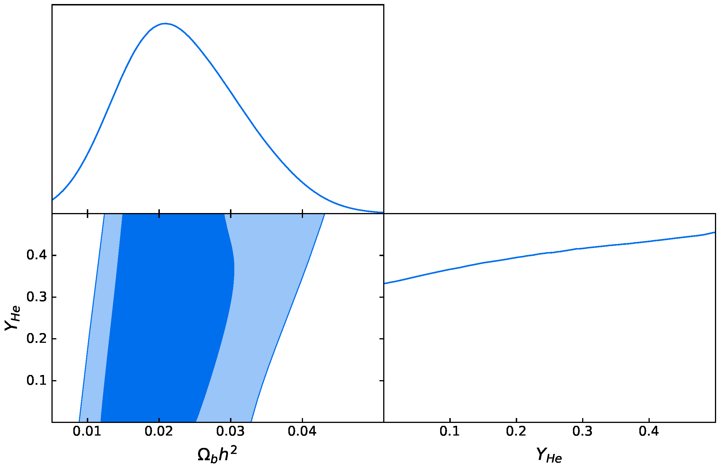
- Then we simulated two mock data: the conservative case at low redshift and the high-redshift case. However, due to the strong degeneracy between the helium abundance and the baryon energy density, the constraints on were still very weak from the mock FRB data.
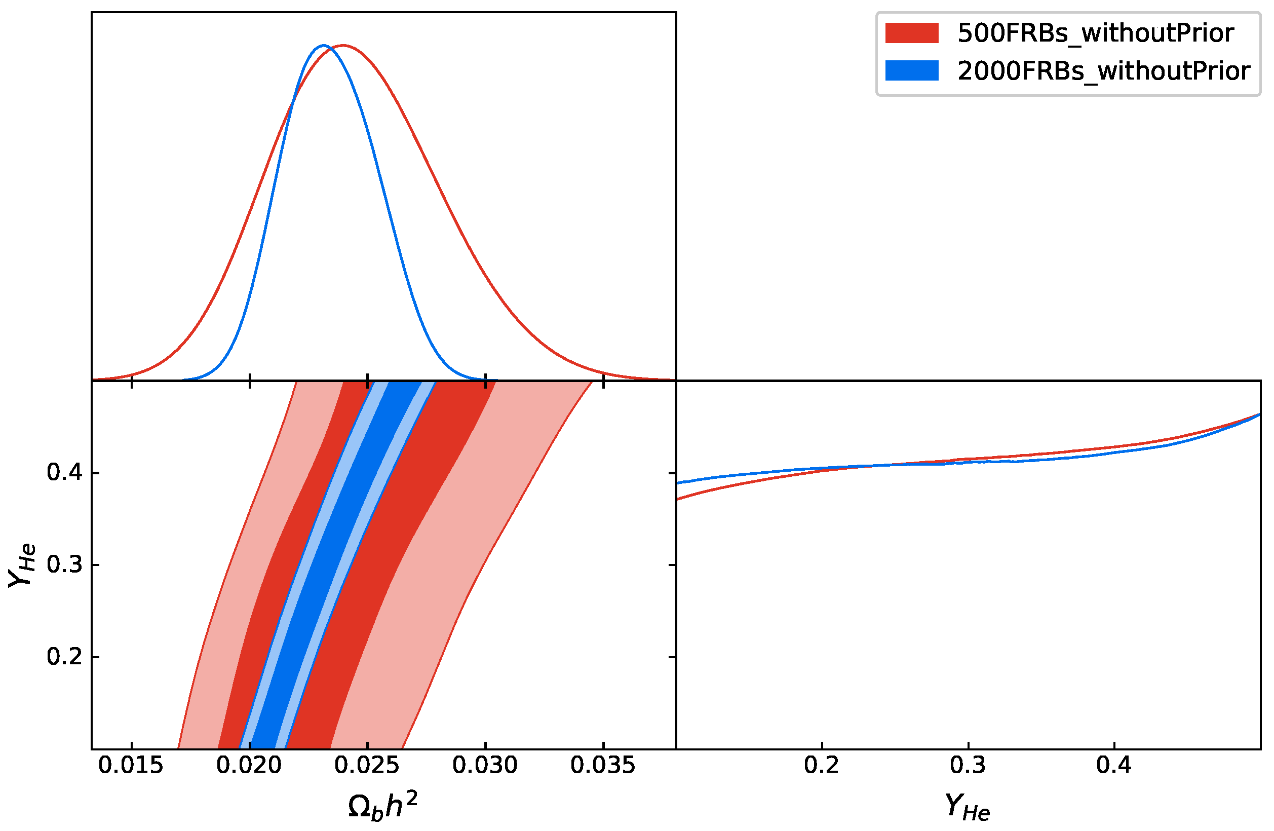
- Therefore, we introduced the distance information of shift parameters, derived from the CMB full power spectra of the Planck measurement. With this help, the constraint on the baryon energy density was significantly improved, and the degeneracy with was broken.
- Consequently, the constraints on the helium abundance were also improved with the standard deviation and for two FRBs’ mock data, respectively. As can be seen from the current CMB constraint at a 95% confidence level and BBN constraint , the constraints from the FRBs are comparable. Hopefully, large FRB samples with high redshift from the Square Kilometre Array will provide high-precision measurements of the helium abundance in the near future.
Author Contributions
Funding
Institutional Review Board Statement
Informed Consent Statement
Data Availability Statement
Acknowledgments
Conflicts of Interest
| 1 | http://frbhosts.org (accessed on 17 April 2022). |
References
- Lorimer, D.R.; Bailes, M.; McLaughlin, M.A.; Narkevic, D.J.; Crawford, F. A Bright Millisecond Radio Burst of Extragalactic Origin. Science 2007, 318, 777. [Google Scholar] [CrossRef] [Green Version]
- Thornton, D.; Stappers, B.; Bailes, M.; Barsdell, B.; Bates, S.; Bhat, N.D.R.; Burgay, M.; Burke-Spolaor, S.; Champion, D.J.; Coster, P.; et al. A Population of Fast Radio Bursts at Cosmological Distances. Science 2013, 341, 53–56. [Google Scholar] [CrossRef] [PubMed]
- Petroff, E.; Bailes, M.; Barr, E.D.; Barsdell, B.R.; Bhat, N.D.R.; Bian, F.; Burke-Spolaor, S.; Caleb, M.; Champion, D.; Chandra, P.; et al. A real-time fast radio burst: Polarization detection and multiwavelength follow-up. MNRAS 2015, 447, 246–255. [Google Scholar] [CrossRef] [Green Version]
- CHIME/FRB Collaboration; Andersen, B.C.; Bandura, K.M.; Bhardwaj, M.; Bij, A.; Boyce, M.M.; Boyle, P.J.; Brar, C.; Cassanelli, T.; Chawla, P.; et al. A bright millisecond-duration radio burst from a Galactic magnetar. Nature 2020, 587, 54–58. [Google Scholar] [CrossRef]
- Metzger, B.D.; Margalit, B.; Sironi, L. Fast radio bursts as synchrotron maser emission from decelerating relativistic blast waves. MNRAS 2019, 485, 4091–4106. [Google Scholar] [CrossRef] [Green Version]
- Kumar, P.; Bošnjak, Ž. FRB coherent emission from decay of Alfvén waves. MNRAS 2020, 494, 2385–2395. [Google Scholar] [CrossRef]
- Lu, W.; Kumar, P.; Zhang, B. A unified picture of Galactic and cosmological fast radio bursts. MNRAS 2020, 498, 1397–1405. [Google Scholar] [CrossRef]
- Vachaspati, T. Cosmic Sparks from Superconducting Strings. Phys. Rev. Lett. 2008, 101, 141301. [Google Scholar] [CrossRef] [Green Version]
- Geng, J.; Li, B.; Huang, Y. Repeating fast radio bursts from collapses of the crust of a strange star. Innovation 2021, 2, 100152. [Google Scholar] [CrossRef]
- CHIME/FRB Collaboration; Amiri, M.; Bandura, K.; Berger, P.; Bhardwaj, M.; Boyce, M.M.; Boyle, P.J.; Brar, C.; Burhanpurkar, M.; Chawla, P.; et al. The CHIME Fast Radio Burst Project: System Overview. ApJ 2018, 863, 48. [Google Scholar] [CrossRef]
- Petroff, E.; Barr, E.D.; Jameson, A.; Keane, E.F.; Bailes, M.; Kramer, M.; Morello, V.; Tabbara, D.; van Straten, W. FRBCAT: The Fast Radio Burst Catalogue. PASA 2016, 33, e045. [Google Scholar] [CrossRef] [Green Version]
- Johnston, K.; Oswalt, T.; Valls-Gabaud, D. Statistical Modeling and Analysis of Wide Binary Star Systems. In Binary Stars as Critical Tools & Tests in Contemporary Astrophysics; Hartkopf, W.I., Harmanec, P., Guinan, E.F., Eds.; Cambridge University Press: Cambridge, UK, 2007; Volume 240, p. 429. [Google Scholar]
- Fialkov, A.; Loeb, A. A Fast Radio Burst Occurs Every Second throughout the Observable Universe. Astrophys. J. Lett. 2017, 846, L27. [Google Scholar] [CrossRef]
- Spitler, L.G.; Scholz, P.; Hessels, J.W.T.; Bogdanov, S.; Brazier, A.; Camilo, F.; Chatterjee, S.; Cordes, J.M.; Crawford, F.; Deneva, J.; et al. A repeating fast radio burst. Nature 2016, 531, 202–205. [Google Scholar] [CrossRef] [Green Version]
- Hagstotz, S.; Reischke, R.; Lilow, R. A new measurement of the Hubble constant using fast radio bursts. MNRAS 2022, 511, 662–667. [Google Scholar] [CrossRef]
- Wu, Q.; Zhang, G.Q.; Wang, F.Y. An 8 per cent determination of the hubble constant from localized fast radio bursts. Mon. Not. R. Astron. Soc. Lett. 2022, slac022. [Google Scholar] [CrossRef]
- Gao, H.; Li, Z.; Zhang, B. Fast Radio Burst/Gamma-Ray Burst Cosmography. ApJ 2014, 788, 189. [Google Scholar] [CrossRef]
- Li, Z.; Gao, H.; Wei, J.J.; Yang, Y.P.; Zhang, B.; Zhu, Z.H. Cosmology-independent Estimate of the Fraction of Baryon Mass in the IGM from Fast Radio Burst Observations. ApJ 2019, 876, 146. [Google Scholar] [CrossRef]
- Dai, J.P.; Xia, J.Q. Reconstruction of baryon fraction in intergalactic medium through dispersion measurements of fast radio bursts. Mon. Not. Roy. Astron. Soc. 2021, 503, 4576–4580. [Google Scholar] [CrossRef]
- Dai, J.P.; Xia, J.Q. Reconstruction of reionization history through dispersion measurements of fast radio bursts. J. Cosmol. Astropart. Phys. 2021, 2021, 050. [Google Scholar] [CrossRef]
- Planck Collaboration; Ade, P.A.R.; Aghanim, N.; Arnaud, M.; Ashdown, M.; Aumont, J.; Baccigalupi, C.; Banday, A.J.; Barreiro, R.B.; Bartlett, J.G.; et al. Planck 2015 results. XIII. Cosmological parameters. Astron. Astrophys. 2016, 594, A13. [Google Scholar] [CrossRef] [Green Version]
- Planck Collaboration; Aghanim, N.; Akrami, Y.; Ashdown, M.; Aumont, J.; Baccigalupi, C.; Ballardini, M.; Banday, A.J.; Barreiro, R.B.; Bartolo, N.; et al. Planck 2018 results. VI. Cosmological parameters. Astron. Astrophys. 2020, 641, A6. [Google Scholar] [CrossRef] [Green Version]
- Aver, E.; Olive, K.A.; Skillman, E.D. The effects of He I λ10830 on helium abundance determinations. J. Cosmol. Astropart. Phys. 2015, 2015, 011. [Google Scholar] [CrossRef] [Green Version]
- Peimbert, A.; Peimbert, M.; Luridiana, V. The primordial helium abundance and the number of neutrino families. Rev. Mexicana Astron. Astrofis. 2016, 52, 419. [Google Scholar]
- Izotov, Y.I.; Thuan, T.X.; Guseva, N.G. A new determination of the primordial He abundance using the He I λ10830 Å emission line: Cosmological implications. MNRAS 2014, 445, 778–793. [Google Scholar] [CrossRef]
- Leath, H.J.; Beasley, M.A.; Vazdekis, A.; Salvador-Rusiñol, N.; Gvozdenko, A. Inferring the helium abundance of extragalactic globular clusters using integrated spectra. MNRAS 2022, 512, 548–562. [Google Scholar] [CrossRef]
- Aver, E.; Olive, K.A.; Porter, R.L.; Skillman, E.D. The primordial helium abundance from updated emissivities. J. Cosmol. Astropart. Phys. 2013, 2013, 017. [Google Scholar] [CrossRef] [Green Version]
- Matsumoto, A.; Ouchi, M.; Nakajima, K.; Kawasaki, M.; Murai, K.; Motohara, K.; Harikane, Y.; Ono, Y.; Kushibiki, K.; Koyama, S.; et al. EMPRESS. VIII. A New Determination of Primordial He Abundance with Extremely Metal-Poor Galaxies: A Suggestion of the Lepton Asymmetry and Implications for the Hubble Tension. arXiv 2022, arXiv:2203.09617. [Google Scholar]
- Deng, W.; Zhang, B. Cosmological Implications of Fast Radio Burst/Gamma-Ray Burst Associations. ApJ 2014, 783, L35. [Google Scholar] [CrossRef] [Green Version]
- McQuinn, M. Locating the “Missing” Baryons with Extragalactic Dispersion Measure Estimates. ApJ 2014, 780, L33. [Google Scholar] [CrossRef] [Green Version]
- Cordes, J.M.; Lazio, T.J.W. NE2001.I. A New Model for the Galactic Distribution of Free Electrons and its Fluctuations. arXiv 2002, arXiv:astro-ph/0207156. [Google Scholar]
- Manchester, R.N.; Hobbs, G.B.; Teoh, A.; Hobbs, M. The Australia Telescope National Facility Pulsar Catalogue. AJ 2005, 129, 1993–2006. [Google Scholar] [CrossRef]
- Macquart, J.P.; Prochaska, J.X.; McQuinn, M.; Bannister, K.W.; Bhandari, S.; Day, C.K.; Deller, A.T.; Ekers, R.D.; James, C.W.; Marnoch, L.; et al. A census of baryons in the Universe from localized fast radio bursts. Nature 2020, 581, 391–395. [Google Scholar] [CrossRef] [PubMed]
- Ioka, K. The Cosmic Dispersion Measure from Gamma-Ray Burst Afterglows: Probing the Reionization History and the Burst Environment. ApJ 2003, 598, L79–L82. [Google Scholar] [CrossRef] [Green Version]
- Kirsten, F.; Marcote, B.; Nimmo, K.; Hessels, J.W.T.; Bhardwaj, M.; Tendulkar, S.P.; Keimpema, A.; Yang, J.; Snelders, M.P.; Scholz, P.; et al. A repeating fast radio burst source in a globular cluster. Nature 2022, 602, 585–589. [Google Scholar] [CrossRef] [PubMed]
- Bhardwaj, M.; Kirichenko, A.Y.; Michilli, D.; Mayya, Y.D.; Kaspi, V.M.; Gaensler, B.M.; Rahman, M.; Tendulkar, S.P.; Fonseca, E.; Josephy, A.; et al. A Local Universe Host for the Repeating Fast Radio Burst FRB 20181030A. ApJ 2021, 919, L24. [Google Scholar] [CrossRef]
- Chatterjee, S.; Law, C.J.; Wharton, R.S.; Burke-Spolaor, S.; Hessels, J.W.T.; Bower, G.C.; Cordes, J.M.; Tendulkar, S.P.; Bassa, C.G.; Demorest, P.; et al. A direct localization of a fast radio burst and its host. Nature 2017, 541, 58–61. [Google Scholar] [CrossRef] [Green Version]
- Marcote, B.; Nimmo, K.; Hessels, J.W.T.; Tendulkar, S.P.; Bassa, C.G.; Paragi, Z.; Keimpema, A.; Bhardwaj, M.; Karuppusamy, R.; Kaspi, V.M.; et al. A repeating fast radio burst source localized to a nearby spiral galaxy. Nature 2020, 577, 190–194. [Google Scholar] [CrossRef]
- Bannister, K.W.; Deller, A.T.; Phillips, C.; Macquart, J.P.; Prochaska, J.X.; Tejos, N.; Ryder, S.D.; Sadler, E.M.; Shannon, R.M.; Simha, S.; et al. A single fast radio burst localized to a massive galaxy at cosmological distance. Science 2019, 365, 565–570. [Google Scholar] [CrossRef] [Green Version]
- Prochaska, J.X.; Macquart, J.P.; McQuinn, M.; Simha, S.; Shannon, R.M.; Day, C.K.; Marnoch, L.; Ryder, S.; Deller, A.; Bannister, K.W.; et al. The low density and magnetization of a massive galaxy halo exposed by a fast radio burst. Science 2019, 366, 231–234. [Google Scholar] [CrossRef] [Green Version]
- Bhandari, S.; Sadler, E.M.; Prochaska, J.X.; Simha, S.; Ryder, S.D.; Marnoch, L.; Bannister, K.W.; Macquart, J.P.; Flynn, C.; Shannon, R.M.; et al. The Host Galaxies and Progenitors of Fast Radio Bursts Localized with the Australian Square Kilometre Array Pathfinder. ApJ 2020, 895, L37. [Google Scholar] [CrossRef]
- Ravi, V.; Catha, M.; D’Addario, L.; Djorgovski, S.G.; Hallinan, G.; Hobbs, R.; Kocz, J.; Kulkarni, S.R.; Shi, J.; Vedantham, H.K.; et al. A fast radio burst localized to a massive galaxy. Nature 2019, 572, 352–354. [Google Scholar] [CrossRef] [PubMed]
- Heintz, K.E.; Prochaska, J.X.; Simha, S.; Platts, E.; Fong, W.f.; Tejos, N.; Ryder, S.D.; Aggerwal, K.; Bhandari, S.; Day, C.K.; et al. Host Galaxy Properties and Offset Distributions of Fast Radio Bursts: Implications for Their Progenitors. ApJ 2020, 903, 152. [Google Scholar] [CrossRef]
- Chittidi, J.S.; Simha, S.; Mannings, A.; Prochaska, J.X.; Ryder, S.D.; Rafelski, M.; Neeleman, M.; Macquart, J.P.; Tejos, N.; Jorgenson, R.A.; et al. Dissecting the Local Environment of FRB 190608 in the Spiral Arm of its Host Galaxy. ApJ 2021, 922, 173. [Google Scholar] [CrossRef]
- Law, C.J.; Butler, B.J.; Prochaska, J.X.; Zackay, B.; Burke-Spolaor, S.; Mannings, A.; Tejos, N.; Josephy, A.; Andersen, B.; Chawla, P.; et al. A Distant Fast Radio Burst Associated with Its Host Galaxy by the Very Large Array. ApJ 2020, 899, 161. [Google Scholar] [CrossRef]
- Day, C.K.; Bhandari, S.; Deller, A.T.; Shannon, R.M.; Moss, V.A. ASKAP localisation of the FRB 20201124A source. Astron. Telegr. 2021, 14515, 1. [Google Scholar]
- Ravi, V.; Law, C.J.; Li, D.; Aggarwal, K.; Burke-Spolaor, S.; Connor, L.; Lazio, T.J.W.; Simard, D.; Somalwar, J.; Tendulkar, S.P. The host galaxy and persistent radio counterpart of FRB 20201124A. arXiv 2021, arXiv:2106.09710. [Google Scholar] [CrossRef]
- Bhandari, S.; Heintz, K.E.; Aggarwal, K.; Marnoch, L.; Day, C.K.; Sydnor, J.; Burke-Spolaor, S.; Law, C.J.; Xavier Prochaska, J.; Tejos, N.; et al. Characterizing the Fast Radio Burst Host Galaxy Population and its Connection to Transients in the Local and Extragalactic Universe. AJ 2022, 163, 69. [Google Scholar] [CrossRef]
- Lewis, A.; Bridle, S. Cosmological parameters from CMB and other data: A Monte Carlo approach. Phys. Rev. D 2002, 66, 103511. [Google Scholar] [CrossRef] [Green Version]
- Qiang, D.C.; Wei, H. Effect of redshift distributions of fast radio bursts on cosmological constraints. Phys. Rev. D 2021, 103, 083536. [Google Scholar] [CrossRef]
- Scóccola, C.G.; Sánchez, A.G.; Rubiño-Martín, J.A.; Génova-Santos, R.; Rebolo, R.; Ross, A.J.; Percival, W.J.; Manera, M.; Bizyaev, D.; Brownstein, J.R.; et al. The clustering of galaxies in the SDSS-III Baryon Oscillation Spectroscopic Survey: Constraints on the time variation of fundamental constants from the large-scale two-point correlation function. MNRAS 2013, 434, 1792–1807. [Google Scholar] [CrossRef] [Green Version]
- Keisler, R.; Reichardt, C.L.; Aird, K.A.; Benson, B.A.; Bleem, L.E.; Carlstrom, J.E.; Chang, C.L.; Cho, H.M.; Crawford, T.M.; Crites, A.T.; et al. A Measurement of the Damping Tail of the Cosmic Microwave Background Power Spectrum with the South Pole Telescope. ApJ 2011, 743, 28. [Google Scholar] [CrossRef]
- Caramete, A.; Popa, L.A. Cosmological evidence for leptonic asymmetry after Planck. J. Cosmol. Astropart. Phys. 2014, 2014, 012. [Google Scholar] [CrossRef]
- Cooke, R.J.; Pettini, M.; Steidel, C.C. One Percent Determination of the Primordial Deuterium Abundance. ApJ 2018, 855, 102. [Google Scholar] [CrossRef] [Green Version]
- Wang, Y.; Mukherjee, P. Observational constraints on dark energy and cosmic curvature. Phys. Rev. D 2007, 76, 103533. [Google Scholar] [CrossRef] [Green Version]
- Li, H.; Xia, J.Q.; Zhao, G.B.; Fan, Z.H.; Zhang, X. On Using the WMAP Distance Information in Constraining the Time-evolving Equation of State of Dark Energy. ApJ 2008, 683, L1. [Google Scholar] [CrossRef] [Green Version]
- Eisenstein, D.J.; Hu, W. Baryonic Features in the Matter Transfer Function. ApJ 1998, 496, 605–614. [Google Scholar] [CrossRef]
- Fialkov, A.; Loeb, A. Constraining the CMB optical depth through the dispersion measure of cosmological radio transients. J. Cosmol. Astropart. Phys. 2016, 2016, 004. [Google Scholar] [CrossRef] [Green Version]


| Name | Redshift | Telescope | Reference | ||
|---|---|---|---|---|---|
| FRB 121102 | 557 | Arecibo | Chatterjee et al. [37] | ||
| FRB 180916 | CHIME | Marcote et al. [38] | |||
| FRB 180924 | ASKAP | Bannister et al. [39] | |||
| FRB 181112 | ASKAP | Prochaska et al. [40] | |||
| FRB 190102 | ASKAP | Bhandari et al. [41] | |||
| FRB 190523 | DSA-10 | Ravi et al. [42], Heintz et al. [43] | |||
| FRB 190608 | ASKAP | Chittidi et al. [44] | |||
| FRB 190611 | ASKAP | Heintz et al. [43] | |||
| FRB 190614 | VLA | Law et al. [45] | |||
| FRB 190711 | ASKAP | Heintz et al. [43] | |||
| FRB 190714 | ASKAP | Heintz et al. [43]) | |||
| FRB 191001 | ASKAP | Heintz et al. [43] | |||
| FRB 200430 | ASKAP | Heintz et al. [43] | |||
| FRB 201124 | ASKAP | Day et al. [46], Ravi et al. [47] | |||
| FRB 180301 | 536 | 152 | Parkes | Bhandari et al. [48] | |
| FRB 191228 | 33 | ASKAP | Bhandari et al. [48] | ||
| FRB 200906 | 36 | ASKAP | Bhandari et al. [48] |
| Mean Value |
Publisher’s Note: MDPI stays neutral with regard to jurisdictional claims in published maps and institutional affiliations. |
© 2022 by the authors. Licensee MDPI, Basel, Switzerland. This article is an open access article distributed under the terms and conditions of the Creative Commons Attribution (CC BY) license (https://creativecommons.org/licenses/by/4.0/).
Share and Cite
Jing, L.; Xia, J.-Q. Constraints on the Helium Abundance from Fast Radio Bursts. Universe 2022, 8, 317. https://doi.org/10.3390/universe8060317
Jing L, Xia J-Q. Constraints on the Helium Abundance from Fast Radio Bursts. Universe. 2022; 8(6):317. https://doi.org/10.3390/universe8060317
Chicago/Turabian StyleJing, Liang, and Jun-Qing Xia. 2022. "Constraints on the Helium Abundance from Fast Radio Bursts" Universe 8, no. 6: 317. https://doi.org/10.3390/universe8060317
APA StyleJing, L., & Xia, J.-Q. (2022). Constraints on the Helium Abundance from Fast Radio Bursts. Universe, 8(6), 317. https://doi.org/10.3390/universe8060317