Article

A Geometric Model in 3+1D Space-Time for Electrodynamic Phenomena

Fakultät für Physik, Technische Universität Wien, Atominstitut, Stadionallee 2, 1020 Wien, Austria
Universe 2022, 8(2), 73; https://doi.org/10.3390/universe8020073
Submission received: 3 December 2021 / Revised: 2 January 2022 / Accepted: 17 January 2022 / Published: 26 January 2022

Abstract

:
With the idea to find geometric formulations of particle physics we investigate the predictions of a three-dimensional generalization of the Sine-Gordon model, very close to the Skyrme model and to the Wu-Yang description of Dirac monopoles. With three rotational degrees of freedom of spatial Dreibeins, we formulate a Lagrangian and confront the predictions to electromagnetic phenomena. Stable solitonic excitations we compare with the lightest fundamental electric charges, electrons, and positrons. Two Goldstone bosons we relate to the properties of photons. These particles are characterized by three topological quantum numbers, which we compare to charge, spin, and photon numbers. Finally, we conjecture some ideas for further comparisons with experiments.

1. Introduction

The standard model of particle physics (SM) and our basic theories, quantum field theory (QFT) and quantum mechanics (QM) are extremely successful. A comparison, excellently suited to demonstrate the high accuracy of these theories, leads to the astonishing agreement between theory and experiment for the gyromagnetic ratio of the electron with a precision of better than 12 digits [1].
On the other hand, there are intensive discussions about the interpretation of QM [2,3,4] and about the mechanisms in nature explaining the phenomena excellently described by the SM. I do not need to repeat here the well-known quote of Feynman about QM. If one reads carefully between the lines of articles and talks of the main builders of the SM, see e.g., the quotes of Veltman and ’t Hooft below, one realizes that they know very well about the interesting open questions. The SM has about 20 real and 10 integer parameters. One cannot expect that these numbers can be explained within the SM.
Galileo has shown us, how to learn from nature, by experiments analyzed with efficient mathematical tools and not by philosophical considerations. There are experiments that may give us some hints in which directions we could try to proceed. Within QM we can describe the properties of spin perfectly, its quantization, and its contribution to angular momentum. It is astonishing, how well we can describe transitions in rotational-vibrational spectra of molecules. But QM does not tell us what is really rotating. The belt-trick and the sphere-trick, see Figure 3 fascinate us with their strange rotation properties which can be mathematically well-understood within the group of rotations SO(3) and may be related to the properties of spin, see Section 3.2.3.
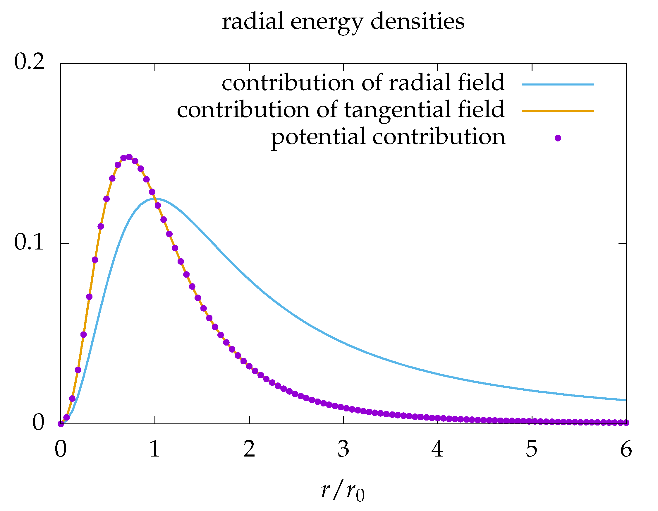
The Sine-Gordon model and its mechanical pendulum models are inspiring since they have solitons, characterized by the topological quantum number Π 1 ( S 1 ) . These solitons behave like particles. Their mass is realized by three contributions to the energy densities of the field: potential, torsion, and kinetic energy. There is a signal velocity c corresponding to the velocity of light. For the mechanical system, it is in the order of m/s. Since the Lagrangian is Lorentz invariant with respect to c we can directly observe Lorentz contraction, in a certain sense making the laws of special relativity visible. The sum of the three energy contributions increases with the gamma-factor corresponding to c, as expected for the mass of a relativistic particle. There are two types of solitons interacting like charges. Solitons and antisolitons have exactly the same properties besides their chirality, resembling the charges of electrons and positrons. Experimentally no differences were found between electrons and positrons, besides the opposite charge. Recent sophisticated experiments show this impressive agreement also for protons and antiprotons [5] with “A 16-parts-per-trillion measurement of the antiproton-to-proton charge–mass ratio”. The Sine-Gordon model [6] gives the inspiration that particles may be characterized by topological quantum numbers, leading to the quantization of charge and to such mirror properties of particles and antiparticles. Even experts in particle physics [7,8,9] raise philosophical questions about the basic entities of QM and QFT. One may see this as an indication that particle physics does not tell us comprehensively enough what particles are. The Sine-Gordon model may give a hint, understandable also for physics laymen.
The interference of electrons in double-slit experiments and of neutrons in interferometers is excellently described by QM. But QM does not give us any understandable idea of how objects, registered in electronic detectors as point-like objects, can interfere with each other. To my knowledge, there is only one experiment that may give us the first idea of how to solve this puzzle, the experiment on bouncing oil-drops invented by Yves Couder [10].
To get a deeper understanding of the phenomena in nature, we can try to construct mathematical models reflecting some of the properties of the above-mentioned experiments. A simple mathematical model of this type I try to discuss in this article. Its main predictions are condensed in Section 5.1. Some of the items mentioned there agree with the experiment and some of them may disagree. Such a disagreement should motivate modifications improving the applicability of the model.
A further aim of this article is to vote for a possible alternative paradigm of particle physics. It is going back to Einstein, who originally tried to unify gravitation and electromagnetism. This philosophy is summarised in the Aftermath.
In his article “More is Different” Philip Anderson [11] remarked that physical sciences can be ordered according to the degree of their fundamentality. The fundamental theory of matter, the Standard Model of Particle Physics, is a complex theory of many fields and their degrees of freedom. One of its cornerstones is quantum chromodynamics with 4 · 8 gluon field degrees of freedom (dofs) and 4 complex fields for every quark type. History taught us that we can describe electromagnetic phenomena with 4 components of the photon field and 4 complex fields for every fundamentally charged particle with coupled linear equations, with Maxwell and Dirac equations. From mathematics, we know that some non-linear equations can be linearized by introducing more dofs. This may lead to the conjecture that the Maxwell-Dirac theory is a clever linearization of a non-linear theory with a smaller number of fields. The disadvantage of linearization may be that they hide the real dynamics.
A problem which bothered electrodynamics for a long time was the infinity of the self-energy of the electron, as was nicely described by Martinus Veltman in a talk at the 65th Lindau Nobel Laureate Meeting in Konstanz, 2 January 2022 fascinate in https://www.mediatheque.lindau-nobel.org/videos/34703/martinus-veltman-discovery-higgs-particle accessed on 2 December 2021. The problem was finally solved by Hendrik Anthony Kramer’s idea of renormalization, by the absorption of infinities in free parameters of the theory. In his talk Veltman commented on the subtraction of two infinities, the bare mass of the electron and the electric self-energy of the electron by the belief of the community: “Maybe at some future time we know more and we know how to deal with these infinities. Maybe we find a better theory, where you go to small distances, maybe something happens there, but we postpone that problem. All we are going to say is whatever we do, the result for the mass of the electron is what we observe and how that comes about, who cares.” A similar statement of Gerard’t Hooft one can read in Ref. [12]: “It was something of a shock to realize that renormalization can end up as an infinite correction to the theory—and yet, it works”. As these statements indicate it may be worthwhile to think about models which give finite results already at the classical level.
One of the big problems of the present status of particle physics is the unification of the interactions. The overwhelming majority of the community thinks that gravitation should be quantized. This article tries to argue for the opposite direction, for a geometrical formulation of electrodynamics moving electrodynamics closer to general relativity. This might lead to a geometrical motivation of charge quantization, similar to the quantization of Dirac monopoles, and reveal a geometrical origin of spin and its quantization. A model of this type was formulated in 1999 [13], but besides an almost one-to-one copy [14] that article was almost completely ignored by the community. Since the author understood since that time several new aspects of the model and since the original presentation was possibly not so easily readable it is time to include the old and new aspects in a revised presentation of the model and compare it to inspiring experiments that have been performed in the last two decades [10,15].
In Section 2 we give the basic definitions of the model, the degrees of freedom (dofs) of the model, and the Lagrangian. In Section 3 we derive the four types of soliton solutions and calculate their energies. These solitons can be characterized by two topological quantum numbers corresponding to charge and spin quantum numbers. In Section 4 we derive the general equations of motion and the energy-momentum tensor. Section 5 separates charges and their fields, compares their relations to Maxwell equations, derives Coulomb and Lorentz forces, demonstrates the geometrical origin of the U(1) gauge invariance, and interprets photons as Goldstone bosons, characterized by a further topological quantum number. Critical questions are asked in Section 6 and some conjectures added. The conclusion starts with short comparisons to related models and enumerates several agreements and differences to Maxwell’s electrodynamics (MEdyn). In the aftermath, the author tries to summarize his understanding in short statements controversial to the present paradigms.

2. Formulation of the Model

We work in Minkowski space-time and derive the dynamics from a Lagrangian. The only degrees of freedom of the model are local spatial Dreibeins at every event which we define by elements of the group of rotations in 3 dimensions, by an SO(3)-valued scalar field. In Einstein’s gravitational theory gravitation is encrypted in the metric tensor, describing a modification of distances and angles in space-time. We aim therefore to describe all long-range properties of nature, i.e., gravitational and electromagnetic, by the properties of space-time. Particles and their fields are formulated by the same degrees of freedom. With the three degrees of freedom of SO(3) we describe electrons and photons and their interaction. Particles are identified by topological quantum numbers of the field of Dreibeins.
Before we specify the dynamics we have to discuss the geometry.

2.1. Geometry

2.1.1. Scalar Field

To simplify the calculations we describe the mentioned rotations by SU(2) elements
Q ( x ) : = q 0 ( x ) i q ( x ) σ with q 0 2 + q 2 = 1 ,
functions of the point x μ in 3D+1 space-time.
The three Pauli matrices i σ k obey the same multiplication rules as the three imaginary quaternionic units and the relation
( σ a ) ( σ b ) = a b + i σ ( a × b ) .
We are using the vector symbol for the three coefficients of the imaginary quaternionic units and of the SU(2) algebra, q σ is a short notation for q i σ i . For simplicity we omit the dot for such three dimensional scalar products, if it does not lead to ambiguities. The × symbol acts always in algebra space.
Since SU(2) which is isomorphic to S 3 is the double covering group of SO(3), field configurations { Q ( x ) | x M 4 } differing by a global center transformation, Q Q , are identical SO(3) configurations. We would like to emphasise that using in Equation (1) the real unit 1 and the three imaginary units i σ k we apply the geometry of R 4 , of the four dimensional euclidean space, to the determination of distances, areas and volumes on the 3-dimensional sphere q 0 2 + q 2 = 1 in 4-dimensions, when we compare them to distances, areas and volumes in M 4 . Another useful parametrisation of Q is
q 0 = : cos α , q : = n sin α , α [ 0 , π 2 ] , n 2 : = 1 n S 2 .
The rotational angle ω corresponding to the SU(2) matrices Q is related to α by ω = 2 α = 2 α n .

2.1.2. Vector Field = Connection Field

The derivatives
μ Q ( x ) = : i Γ μ ( x ) σ Q ( x )
map the pair x , μ to tangential vectors on the SU(2)-manifold. The connection coefficients Γ μ between neighbouring Dreibeins can be expressed by the parameters in Equation (3)
Γ μ = ( 6 ) ( 4 ) q 0 μ q q μ q 0 + q × μ q = ( 3 ) n μ α + sin α cos α μ n + sin 2 α n × μ n ,
where we have used
μ Q Q = ( 1 ) ( μ q 0 i σ μ q ) ( q 0 + i σ q ) = ( 2 ) q 0 μ q 0 + q μ q 0 i σ ( q 0 μ q q μ q 0 + q × μ q )
For the description of electro-magnetic phenomena we relate the geometrical quantity Γ μ to a dual non-abelian vector potential
C μ : = e 0 4 π ε 0 c 0 Γ μ ,
where e 0 is the fundamental electric charge unit, ε 0 the dielectric constant and c 0 the velocity of light.
The derivatives of vectors in algebra space define the covariant derivate
μ v ( x ) : = μ [ σ Q ( x ) v ( x ) ] = ( 5 ) σ μ Q ( x ) v ( x ) i [ v ( x ) σ ] [ Γ μ ( x ) σ ] Q ( x ) + σ Q ( x ) μ v ( x ) = = ( 2 ) i Q ( x ) Γ μ ( x ) v ( x ) + σ [ v ( x ) × Γ μ ( x ) ] Q ( x ) + σ Q ( x ) μ v ( x ) = = i Q ( x ) Γ μ ( x ) v ( x ) radial + σ Q ( x ) [ μ Γ μ ( x ) × ] v ( x )
We assume double differentiable scalar fields and apply Schwarz’s theorem
μ ν Q ( x ) = ν μ Q ( x ) .
From the corresponding expressions
μ ν Q ( s , t ) = ( 4 ) μ ( i σ Γ ν Q ) = ( i σ Γ ν ) ( i σ Γ μ ) Q μ Γ ν i σ Q = ( 2 ) Γ ν Γ μ Q ( μ Γ ν + Γ ν × Γ μ ) i σ Q , ν μ Q ( s , t ) = Γ μ Γ ν Q ( ν Γ μ + Γ μ × Γ ν ) i σ Q ,
we get the Maurer-Cartan equation
μ Γ ν ν Γ μ = ( 10 ) ( 9 ) 2 Γ μ × Γ ν ,
which describes that the 4 × 3 vector field components are derived from a unique SU(2) scalar field with 3 degrees of freedom only.

2.1.3. Curvature Field

Unit squares in M 4 are mapped to parallelograms in the tangential space of S 3 with the area vector
R μ ν : = Γ μ × Γ ν = ( 11 ) 1 2 ( μ Γ ν ν Γ μ ) .
Using these two expressions for R μ ν we can write it in a more general form
R μ ν = ( 12 ) μ Γ ν ν Γ μ Γ μ × Γ ν .
which reminds of the components of the (gauge covariant) field strength tensor in SU(2)-QCD and of the curvature tensor in general relativity.
At a first glance readers may draw the wrong conclusion that μ Q Q in Equation (4) defines a trivial connection. A trivial connection A μ one would get by μ Q Q = : i A μ ( x ) σ 2 , differing slightly from Equation (4). Inserting the relation between A μ and Γ μ , A μ = 2 Γ μ , to Equation (11) shows that the two-form
μ A ν ν A μ A μ × A ν = ( 11 ) 0
is vanishing identically and therefore useless for a determination of areas on S 3 .
Here we can also observe the geometrical realization of gauge transformations, Γ μ Γ μ , as basis changes in the three-dimensional euclidean tangential space at Q. R μ ν σ Q is a vector in this three-dimensional tangential space at Q on S 3 , represented by the special basis vectors σ i Q . In this special gauge, the algebraic expression for R μ ν is defined by Equation (12). After a basis change the affine connection is modified, Γ μ Γ μ , and Equation (12) cannot be used anymore. As one can see, performing the basis change explicitly, the more general Equation (13) is still valid after arbitrary basis rotations in the tangential space at Q, after arbitrary local gauge transformations.
We relate the curvature field R μ ν to dual non-abelian field strength tensor components by
e 0 4 π ε 0 c 0 R μ ν = : 1 2 ε μ ν ρ σ F ρ σ = : F μ ν = 0 B 1 B 2 B 3 B 1 0 E 3 c 0 E 2 c 0 B 2 E 3 c 0 0 E 1 c 0 B 3 E 2 c 0 E 1 c 0 0 .
where we used the convention ε 0123 = 1 for the total antisymmetric epsilon tensor.
It may be astonishing, why we decided to use this dual representation to describe electric charges, though a short calculation shows that the abelian j el ν and the non-abelian electric current J el ν vanish
j el ν : = μ F μ ν ϵ μ ν ρ σ μ R ρ σ = ( 8 ) ϵ μ ν ρ σ μ ρ Γ σ 0 = 0 .
J el ν : = D μ F μ ν ϵ μ ν ρ σ D μ R ρ σ = ( 12 ) ( 8 ) ϵ μ ν ρ σ μ ρ Γ σ j el ν 1 2 ϵ μ ν ρ σ Γ μ × R ρ σ = = ϵ μ ν ρ σ μ ρ 0 Γ σ 1 2 ϵ μ ν ρ σ Γ μ × ( Γ ρ × Γ σ ) Γ ρ ( Γ μ Γ σ ) Γ σ ( Γ μ Γ ρ ) = 0 .
The zeroth component of these equations forbids the existence of non-abelian electric sources
D i E i = ( 17 ) i E i = ( 17 ) 0 .
But this does not mean that the abelian electric flux lines are closed. They have sources, the topological solitons of this model.
Already here we would like to mention that in this description with dual vector fields static charges are formulated with spatial components of static vector fields (5). For moving charges and for their magnetic fields F 0 i R 0 i non-vanishing time-components of the connection Γ μ are necessary.
After the definition of the geometrical quantities, we are ready to define the dynamics.

2.2. Lagrangian

To keep solitons stable we need besides the almost familiar term L curv , quadratic in the field strength, a potential term L pot
L : = L curv + L pot : = α f c 0 4 π 1 4 R μ ν R μ ν + Λ ( q 0 ) with Λ ( q 0 ) : = q 0 6 r 0 4 .
The prefactor of L curv we have formulated with Sommerfeld’s fine structure constant α f : = e 0 2 4 π ε 0 c 0 [SI] in order to use an expression which is valid in SI and in the cgs unit system. In more familiar terms the square term reads in SI units
L curv = ( 15 ) ( 19 ) 1 4 μ 0 F μ ν F μ ν = ( 15 ) ϵ 0 2 E E + 1 2 μ 0 B B ,
with ε 0 μ 0 c 0 2 = 1 . As we will discuss in Section 3 this Lagrangian allows for 4 types of stable solitons with long range, Coulombic interaction. Since we want to compare the properties of these solitons with experiments, we compare them to the lightest monopoles existing in nature, with electrons. This is the reason why we relate R μ ν to F μ ν . The sign of L curv does not matter for a classical system. It decides whether quantum fluctuations are suppressed.
We would like to mention that up to the multiplicative constant α f , L curv is geometrically identical to the Skyrme term in the Skyrme model [16,17], with the distinction that the Skyrme model is using the vanishing field strength tensor (14) and describes solitons with short-range interaction which are interpreted as baryons.
L curv tends to expand solitons. To stabilize solitons we need a further term in the Lagrangian, a compression term with a smaller number of derivatives. A term, quadratic in the derivatives, as used by Skyrme, forbids solitons with long-range interaction. A basic idea of our model is to have solitons with a hedgehog field extending to infinity and covering only half of S 3 . This can only be achieved with a potential term Λ ( q 0 ) without derivatives and the minimum at q 0 = 0 , at the equator of S 3 . Λ ( q 0 ) = q 0 6 / r 0 4 turned out to lead to the simplest solution, and it is appealing to believe that the simplest solution is also the most natural, even if one does not know yet its origin. The factor r 0 4 is necessary for dimensional reasons. r 0 is the length scale responsible for the size and the mass of solitons. Fixing q 0 to 0 keeps the two dynamical degrees of freedom encoded in the n -field, see Equation (3), and leads to a symmetrical broken vacuum. It allows for two massless excitations which can be related to the two massless excitations of electrodynamics, to photons, see Section 5.4.
This definition of the Lagrangian leads to three topological quantum numbers, π 2 ( S 2 ) , π 3 ( S 3 ) and π 3 ( S 2 ) which we will relate to the topological quantization of electric charge, spin, and photon number, as will be discussed in Section 3.2 and Section 5.4.
We are looking for stable static solutions of the equations of motion. The two terms in the Lagrangian (19) differ in the number of derivatives leading to a difference in the scale dependence, x λ x
H cur : = ( 20 ) ϵ 0 2 d 3 x E i E i 1 λ H cur , H pot : = ( 19 ) α f c 0 4 π d 3 x q 0 6 r 0 4 λ 3 H pot .
For stable minima of the total energy
H tot : = H cur + H pot
we get therefore a relation between the corresponding static energy contributions
d d λ H tot | λ = 1 = ( 22 ) d d λ H cur | λ = 1 + d d λ H pot | λ = 1 = ( 21 ) H cur + 3 H pot = 0 .
In Section 3 we can check the validity of this application of the Hobart-Derrick theorem [18,19] for the analytical solution.

3. Soliton Solutions

3.1. Hedgehog Solution

We expect to find a spherical symmetric soliton with the shape of a hedgehog, see Figure 1, and use the parameters (3) to define the spherically symmetric hedgehog
n i ( x ) : = x i r , α ( r ) [ 0 , π 2 ] α ( 0 ) = 0 , α ( ) = π / 2 .
From the soliton field Q ( x ) we get the connection coefficients
Γ r = ( 5 ) n r α , Γ ϑ = ( 5 ) sin α cos α e θ + sin α e ϕ = : sin α e ξ , Γ φ = ( 5 ) sin ϑ sin α cos α e ϕ sin α e θ = : sin ϑ sin α e η ,
where n , e θ , e ϕ and e ξ : = cos α e θ + sin α e ϕ , e η : = cos α e ϕ sin α e θ are spherical unit vectors in the su(2) algebra.
For the determination of the dual vector potential from the geometrical quantity Γ μ we have to take into account the length scales in spherical coordinates ( l r , l ϑ , l φ ) = ( 1 , r , r sin ϑ )
C r = ( 7 ) e 0 4 π ε 0 c 0 Γ r l r , C ϑ = e 0 4 π ε 0 c 0 Γ ϑ l ϑ , C φ = e 0 4 π ε 0 c 0 Γ φ l φ .
We would like to mention, that due to the dual formulation and in distinction to Maxwell’s electrodynamics (MEdyn) only the spatial components Γ i , i { 1 , 2 , 3 } of the vector field Γ μ are involved in the description of static charges. In this way, static problems are described with static fields and spatial derivatives. Time-dependent problems need time-dependent fields and time derivatives.
Up to the measure system depending constant e 0 4 π ε 0 , the electric field strength is given by the ratio of an area in the tangential space of S 3 divided by the corresponding area at ( r , ϑ , φ ) in 3-dimensional (3D) space
E r = ( 15 ) ( 12 ) e 0 4 π ε 0 Γ ϑ × Γ φ r 2 sin ϑ = ( 26 ) e 0 4 π ε 0 sin 2 α r 2 n r e 0 4 π ε 0 1 r 2 n , E ϑ = e 0 4 π ε 0 Γ φ × Γ r r sin ϑ = e 0 4 π ε 0 sin α r α r e ξ r 0 , E φ = e 0 4 π ε 0 Γ r × Γ ϑ r = e 0 4 π ε 0 sin α r α r e η r 0 .
From α ( r ) r π / 2 we get sin α ( r ) 1 and r α ( r ) 0 . Only the radial electric field strength survives for large r and approaches zero like r 2 . Its abelian part gets asymptotically the intended result 1
E n r 1 4 π ε 0 e 0 r 2 r r .
The shape of the profile function α ( r ) follows from a minimisation of the total energy
H tot = ( 3 ) ( 22 ) d 3 r ε 0 2 ( E r E r + E ϑ E ϑ + E φ E φ ) + α f c 0 4 π cos 6 α r 0 4 = = ( 27 ) α f c 0 0 d r sin 4 α 2 r 2 + ( r cos α ) 2 + r 2 r 0 4 cos 6 α = = α f c 0 r 0 0 d ρ sin 4 α 2 ρ 2 + ( ρ cos α ) 2 + ρ 2 cos 6 α with ρ : = r r 0 ,
where r 0 defines the scale for the size and the mass of the soliton. The first term in the final energy expression is due to the radial electric field, the second due to the two tangential fields and the third due to the potential energy.
By the variation of the energy functional (29) with respect to α ( ρ ) we get the differential equation for the minimum of the energy
( 1 cos 2 α ) cos α ρ 2 + ρ 2 cos α 3 ρ 2 cos 5 α = 0 ,
a nonlinear differential equation of second order. This equation is fulfilled by
α = ( 30 ) arctan ρ = arctan r r 0 .
With
sin α ( r ) = ρ 1 + ρ 2 cos α ( r ) = 1 1 + ρ 2 ,
we get the three contributions to the radial energy density, the r dependent spherical integrals in Equation (29),
h = ( 29 ) α f c 0 r 0 ρ 2 2 ( 1 + ρ 2 ) 2 + ρ 2 ( 1 + ρ 2 ) 3 + ρ 2 ( 1 + ρ 2 ) 3
listed in the same order as in Equation (29). They are depicted in Figure 2 without the prefactor α f c 0 r 0 .
The integrals over these radial energy densities behave as 2:1:1 and lead to the total energy
H tot = α f c 0 r 0 π 4 .
The ratio 2:1 between radial and tangential energies is specific to the chosen power in the potential energy. The ratio 4:1 between total energy and potential energy contribution is due to the Hobart-Derrick theorem, see Equation (23). We can try to fix the parameter r 0 of the model by a comparison with experiments. The only known fundamental stable monopoles are electrons with a self-energy of 0.511 MeV. This comparison leads to
r 0 = 2.21 fm .
It is in the order of the classical electron radius r cl : = α f c 0 m e c 0 2 = 2.82 fm.
The stable soliton configuration, derived in this section, is tightly related to the monopoles which Dirac invented [20,21], to describe magnetic monopoles within MEdyn. Dirac monopoles have two types of singularities, a Dirac string which is necessary to allow for a non-vanishing magnetic charge, and a singularity in the center well-known for all point-like charges in MEdyn. Due to the presence of the quantized string, Dirac monopoles have quantized magnetic charges. Wu and Yang [22,23] found another representation of point-like Dirac monopoles by a normalized n -field of the same structure as defined in Equation (24) where the Dirac string is removed and the singularity in the center is still existing. This point-like singularity warrants the quantization of magnetic charges. In this article, we emphasize that one should regularize this central singularity by enlarging the degrees of freedom to an SU(2) scalar field and defining a Lagrangian that stabilizes such monopole configurations. With these modifications and a dual interpretation of the fields, one gets a classical field theory for Dreibeins in space-time which has many features well-known from classical electrodynamics. It is an interesting subject to investigate which predictions of this dual formulation of electrodynamics differ from Maxwell’s electrodynamics (MEdyn) and which predictions disagree with the experiments to electrodynamics (Edyn).

3.2. Quantum Numbers of Solitons

The topological structure of solitons is characterized by discrete, integer, or half-integer topological quantum numbers. They lead to integer charges, half-integer spin quantum numbers, integer photon numbers, and to the astonishing mirror properties of particles and antiparticles.

3.2.1. Charge

One can classify field configurations mapping spheres to spheres. Spatial infinity is isomorphic to S 2 . The field of a single soliton at the spatial infinity S 2 is characterised by q 0 = 0 and varying n -field depending on the spatial direction and covering the equatorial S equ 2 of S 3 . The map Π 2 ( S 2 ) : S 2 S equ 2 of Equation (24) is characterised by the winding number Z = 1 which we can relate to the electric charge Q el of the soliton by
Q el : = e 0 Z .
In the limit r 0 0 an arbitrary smooth SU(2)-valued scalar field reduces to a scalar n -field with n 2 = 1 , i.e., an S 2 -field, with Dirac monopoles in the Wu-Yang representation [22,23]. This justifies to define the charge number Z enclosed in a connected volume V with a surface V isomorphic to S 2 by the topological quantum number associated to the map Π 2 ( S 2 )
Z ( V ) : = 1 4 π S ( u , v ) d u d v n [ u n × v n ]
where we parametrised the surface by two parameters u and v, e.g., ϑ and φ .

3.2.2. Topological Charge

The hedgehog solution found in Section 3.1 is characterised by a further quantum number, the number of coverings of the SU(2) manifold, the topological charge
Q : = 1 2 π 2 0 d r 0 π d ϑ 0 2 π d φ Γ r ( Γ ϑ × Γ φ ) = 1 2 π 2 d 3 r Γ x ( Γ y × Γ z ) .
Γ x ( Γ y × Γ z ) is here the Jacobi determinant for the map of the three dimensional space to S 3 . 2 π 2 is the volume of S 3 , therefore Q = 1 describes a full covering. The hedgehog configuration (24) covers only half of S 3 resulting in Q = 1 2 .
By Poincaré transformations we remain in the same topological sector as long as we restrict them to translations, rotations and boosts, since they belong to the connected component of the identity. By parity transformations Π n and transformations with the non-trivial center element z = 1 of SU(2)
Π n : n n , Q = q 0 i n σ sin α Q = q 0 + i n σ sin α x
z : Q Q x
we can get topologically stable monopole configurations differing in the topological quantum numbers Z and Q , enumerated in Table 1.
Configurations with vectors q pointing outwards/inwards are characterized by Z = + 1 / 1 , respectively. Crossing the center of the configurations in an arbitrary direction leads to a rotation by ± 2 π . We get a right-handed rotation, 2 π , for the configurations with Q = 1 2 and a left-handed rotation, 2 π , for Q = 1 2 . With the sign of Q we define an internal chirality χ and with the absolute value of Q the spin quantum number s,
Q = χ · s with s : = | Q | .
The spin quantum number of two-soliton configurations indicated that χ can be related to the sign of the magnetic spin quantum number.
Equation (41) may possibly give an answer to a question which T.D.Lee posed in a talk at the University of Vienna around 1990: “Why does mass violate chiral symmetry?”
Motivated by the definition. (38) we introduce the topologcial current
k μ : = ϵ μ ν ρ σ 12 π 2 Γ ν ( Γ ρ × Γ σ ) = ϵ μ ν ρ σ 24 π 2 Sp [ ( i σ Γ ν ) ( i σ Γ ρ ) ( i σ Γ σ ) ] = = ( 4 ) ϵ μ ν ρ σ 24 π 2 Sp [ ν Q Q ρ Q Q σ Q Q ] = ϵ μ ν ρ σ 24 π 2 Sp Q ν Q ρ Q σ Q
Regions of k μ 0 turn out to be identical to regions with L pot 0 . k μ is obviously a conserved current
μ k μ = ( 42 ) ϵ μ ν ρ σ 12 π 2 Sp μ Q ν Q ρ Q σ Q = = ϵ μ ν ρ σ 12 π 2 Sp μ Q Q ν Q Q ρ Q Q σ Q Q = 0 .
If a soliton is leaving the investigated volume the topological charge will change. The conservation of k μ has the interesting consequence of vanishing F μ ν F μ ν E B ,
0 = ( 43 ) ϵ μ ν ρ σ Sp μ Q Q ν Q Q ρ Q Q σ Q Q = = ( 4 ) ϵ μ ν ρ σ Sp [ ( i σ Γ μ ) ( i σ Γ ν ) ( i σ Γ ρ ) ( i σ Γ σ ) ] = = 2 ϵ μ ν ρ σ ( Γ μ × Γ ν ) ( Γ ρ × Γ σ ) = 2 ϵ μ ν ρ σ R μ ν R ρ σ F μ ν F μ ν .
The four configurations of Table 1 correspond to the four components of Dirac spinors, spin up ↑ and down ↓, electron e and positron e + . In the order of Table 1 we can attribute to the configurations the particle types and spin components
e , e + , e , e +
In relativistic quantum mechanics, we can attribute to particles an intrinsic parity and use γ 0 as a parity operator. The Dirac equation has two pairs of solutions of opposite parity. This abstract parity property has an anschauliche realization in the figures of Table 1 with two pairs of configurations with opposite parity.

3.2.3. Spin as Angular Momentum

Spin properties are well-known in quantum mechanics. They are understood as internal properties of particles, characterized by the spin quantum number s taking half-integer values as described by the group SU(2) and its representations. Similar, but more general quantization rules, those of SU(3), are known for the color of quarks. In distinction to the internal color property in QCD and the Standard Model, spin contributes to the total angular momentum. This property is the origin of one of the enigmas of quantum mechanics, since this fundamental theory does not tell us what is really rotating, especially due to the point-like nature of fundamental particles which is generally assumed. Further, the spin is associated with a contribution to the magnetic moment of particles which in all other circumstances has its origin in the motion of charges.
It is an interesting question whether the present model may lead to some deeper understanding of these riddles. It seems obvious that stable SO(3) field configurations covering half of the SU(2) group manifold follow the quantization rules of SU(2) for the defining two-dimensional representation and its tensor products.
In fact, we can see that we can combine the four single-particle configurations of Table 1 to 4 3 = 10 topologically different configurations. The charge numbers Z = ± 1 combine to Z = 0 or ± 2 and the topological charges Q = ± 1 / 2 to Q = 0 or Q = ± 1 . The combination has to be done by appropriate rotations of one of the single-particle configurations. In this way, it is possible to merge the two different configurations and to minimize the energy, fixing the centers of the solitons, as will be described in more detail in a forthcoming paper. In the framework of our SO(3)-model, we have to respect that configurations differing in the sign of Q are physically identical. In Figure 3 we show schematic diagrams for two configurations with Z = 0 . They are axially symmetric around the vertical axis. The vectors q of the imaginary parts of the soliton field are plotted. The left diagram with q 0 0 everywhere and spin quantum number s = 0 differs slightly from the right diagram for s = 1 , with q 0 0 in the upper half and q 0 0 in the lower half for this attractive configuration. Comparing the single-particle configurations in Table 1 with Figure 3 one can observe that in the lower soliton configurations, the antiparticles are rotated by π around the vertical symmetry axis. For comparison, some electric field lines are drawn. They agree with lines n = const. This agreement can be used to find an appropriate initial configuration for a minimization process.
A very famous property of spin-1/2 particles is their 4 π -periodicity under rotations. It is well-known in mathematics, even if not all mathematicians and physicists know about it: Objects which are connected with a fixed surrounding feel this 4 π -periodicity. This can easily be shown in a nice tiny experiment with an around decimetre sized sphere which is connected by stretchable rubber bands with a surrounding 3-dimensional frame. After a 2 π -rotation these wires are terribly entangled and even more after a 4 π -rotation, but then the wires can be nicely disentangled without further moving the central sphere by some skillful movements of the wires. More regularly this is shown in Figure 4 where the rotation angle of the inner sphere increases from left to right from 0 to 4 π , as indicated by the red dot rotating around the black dot where the rotational axis pierces. The other shells and their piercings perform rigid rotations around varying axes. The sets of these rotations build lassos on S 3 contracting from inside to outside from a big circle to a point.
Exactly this 4 π -periodicity is shared by the soliton configurations in Table 1 which are connected to the sphere at spatial infinity by imaginary rubber bands of constant n -vectors. This may be a hint that spin-1/2 particles may be extended objects, connected to the surrounding by some fields, e.g., electrons by their electric field lines.
In the first moment it may be disturbing to compare the discussed stable soliton solutions with electrons, since these stable solutions have no internal angular momentum and no magnetic moment, they are just static and spherically symmetric. But, in this soliton model spin angular momentum appears as a consequence of orbital motion. The fact that orbital motion leads to internal rotation can easily be shown in an animation of such a rotation. It is a pity that it is difficult to show this behavior in an article. To give an impression, two of such diagrams are shown in Figure 5 and can be compared to Figure 3b.
The internal rotation of the two solitons can be observed in the region of the two circles. It is caused by the broken symmetry of the vacuum with Q = i σ ( 0 , 0 , 1 ) , approached by the soliton field at large distances for integer topological charges Q . It forces the center of the solitons to rotate with the same frequency in the opposite direction. The two different colors indicate q 0 > 0 and q 0 < 0 . As well-known from quantum mechanics, the internal angular momentum has a fixed relation to the orbital angular momentum, the speed of the internal rotation can not be enlarged or diminished. It will be interesting to compare the internal angular momentum to the orbital angular momentum in analytical or numerical calculations. There is an energy difference between the configurations for s = 0 and s = 1 which should contribute to the spin-orbit interaction.
Just like spin angular momentum, the magnetic moment is in this model a dynamical property, a reaction to external magnetic fields. Such magnetic fields with sources in external moving charges should be encoded in the periodic time dependence of the soliton field in the “vacuum”. These external fields may lead to internal rotation of solitons and to orbital motion.
Dipole configurations of soliton pairs with opposite charge numbers are unstable due to Coulomb attraction. They can be stabilized in numerical simulations, fixing the position of the soliton centers. In several diploma theses [24,25,26] it turned out that the numerical minimization of dipole configurations suffers from a numerical instability making it difficult to avoid the annihilation of dipoles with small separations. It is caused by the instability of single monopole configurations due to numerical errors. This problem was solved in [27] and the accuracy of the solution tested for single monopoles in [28].

4. General Equations of Motion

Equation (30) is the differential equation which results from the Lagrangian (19) for a static spherical symmetric configuration. For a general field configuration we get the momentum density (52) and the Euler-Lagrange Equation (53) by a variation of the soliton field Q
Q Q : = e i σ ζ Q = ( 1 ) 1 i σ ζ ( q 0 i q σ ) = = q 0 ζ q i σ q + q 0 ζ + ζ × q .
We get up to first order in ζ
δ q 0 = ζ q
δ Γ μ = ( 4 ) i 2 Sp { [ μ ( Q + δ Q ) ( Q + δ Q ) μ Q Q ] σ } = μ ζ 2 Γ μ × ζ
δ R μ ν = ( 12 ) μ ζ × Γ ν + 2 Γ μ ( ζ Γ ν ) ν ζ × Γ μ 2 Γ ν ( ζ Γ μ ) .
From Γ ν R μ ν = ( 12 ) 0 follows for the square of the curvature
δ ( R μ ν R μ ν ) = 2 δ R μ ν R μ ν = ( 49 ) 4 ( μ ζ × Γ ν ) R μ ν = 4 μ ζ ( Γ ν × R μ ν ) .
From the variation of the Lagrange density (19)
4 π α f c 0 δ L = ( 19 ) δ 1 4 R μ ν R μ ν + Λ ( q 0 ) = ( 47 ) ( 50 ) ( ζ q ) q 0 Λ + μ ζ ( Γ ν × R μ ν )
we read the momentum density
π μ : = L μ ζ = ( 51 ) α f c 0 4 π Γ ν × R μ ν = ( 19 ) L Γ μ .
The last expression for π μ shows that Γ μ can be regarded as generalised velocity. Further we get the general equation of motion
μ [ Γ ν × R μ ν ] + q d Λ d q 0 = ( 50 ) 0 μ π μ + q d L pot d q 0 = ( 50 ) 0
describing that the variation of the potential is the source of the momentum current. With R μ ν = ( 13 ) ( 12 ) 1 2 ( μ Γ ν ν Γ μ ) and R μ ν × R μ ν = 0 we can get another form of the equation of motion
Γ ν × μ R μ ν + q d Λ d q 0 = 0 .
A consequence of the equation of motion is
Γ ν μ π μ = ( 53 ) Γ ν q d L pot d q 0 = ( 5 ) ν α sin α d L pot d q 0 = ( 3 ) ν q 0 d L pot d q 0 = ν L pot .
In Section 5 we will separate the system into point-like sources and their fields. This should allow some checks whether these equations describe the dynamics of these solitons and their interactions with electromagnetic fields correctly.
Using the generalised velocity Γ μ it is easy to derive the energy momentum tensor
Θ μ ν ( x ) : = L ( x ) Γ μ Γ ν L ( x ) δ ν μ = ( 52 ) π μ Γ ν L ( x ) δ ν μ = = ( 12 ) ( 52 ) α f c 0 4 π Γ ν × Γ σ Γ μ × Γ σ L ( x ) δ ν μ .
In distinction to the energy momentum tensor in Maxwell’s theory, it is automatically symmetric. Its trace is determined by the potential energy
Θ μ μ = ( 19 ) ( 56 ) 4 L pot = ( 19 ) α f c 0 4 π Λ ( q 0 ) .
The force density is given by the divergence of the energy momentum tensor
f ν : = μ Θ ν μ = ( 56 ) Γ ν μ π μ + μ Γ ν π μ ν Γ μ π μ 2 R μ ν π μ ν L pot = = ( 12 ) Γ ν μ π μ + 2 R ν μ π μ ν L pot = ( 55 ) 2 R ν μ π μ = ( 12 ) ( 52 ) 0 ,
where we used R ν μ π μ = 0 . It is finally not astonishing that the force density vanishes in a classical closed system.
To identify the forces between particles and their fields one has to separate artificially particles from fields. This will be done in the next section.

5. Electrodynamic Limit

In the limit r 0 0 the energy of solitons approaches infinity, we dubbed it the electrodynamic limit [29]. It suffers from the problem of infinities of the selfenergy of point-like charges, well-known from Maxwell’s electrodynamics. Within these models, the only known solution is Kramers suggestion to subtract compensating infinities. In this limit, we do not care about these infinities and arrive at the Wu-Yang formulation of Dirac monopoles [22,23]
Q ( x ) : = i σ n ( x ) , n 2 : = 1 , q : = n , q 0 : = cos α = 0 , α : = π 2 ,
with values of the soliton field n ( x ) on S 2 . We use the singularities of the
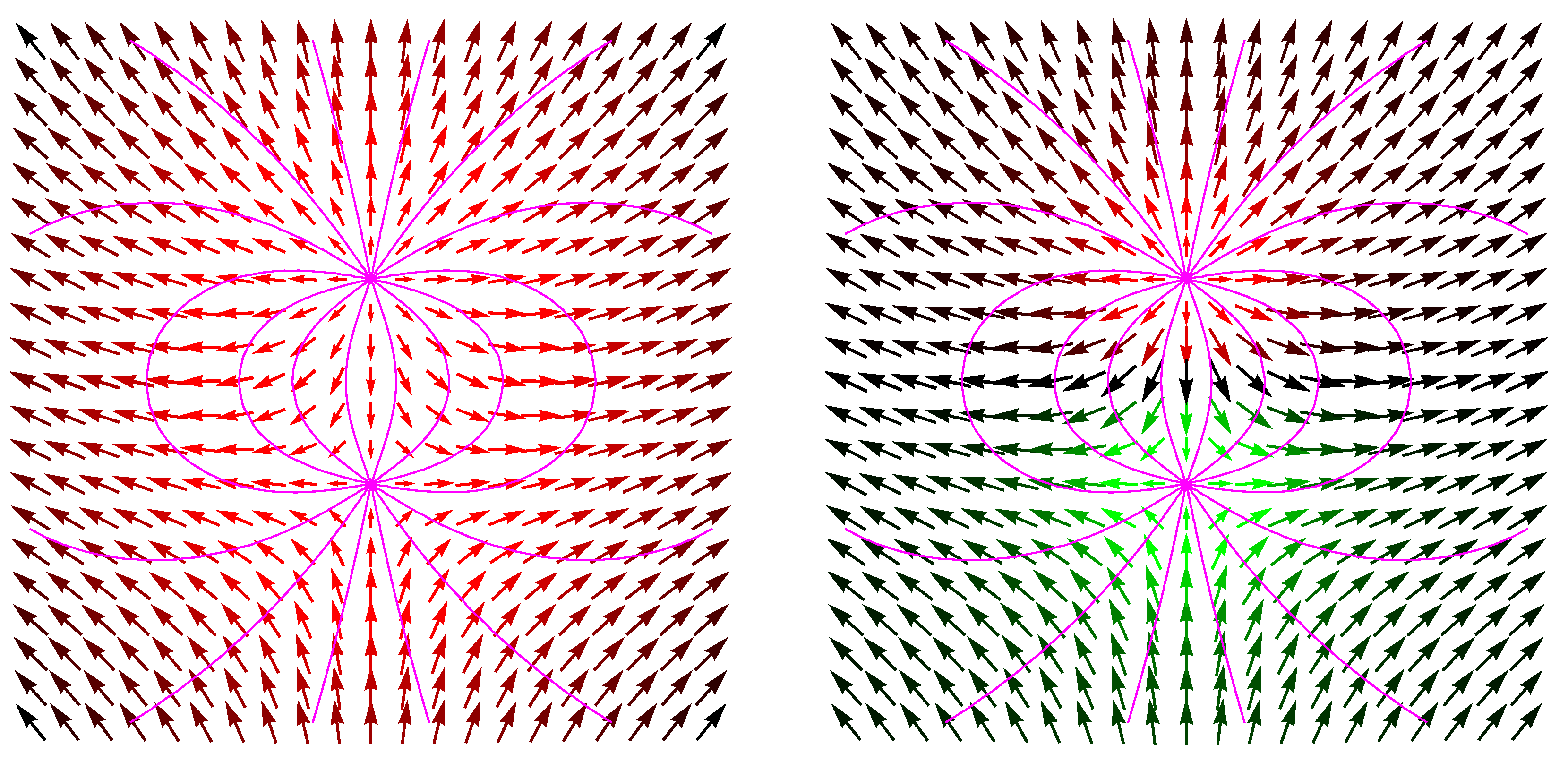
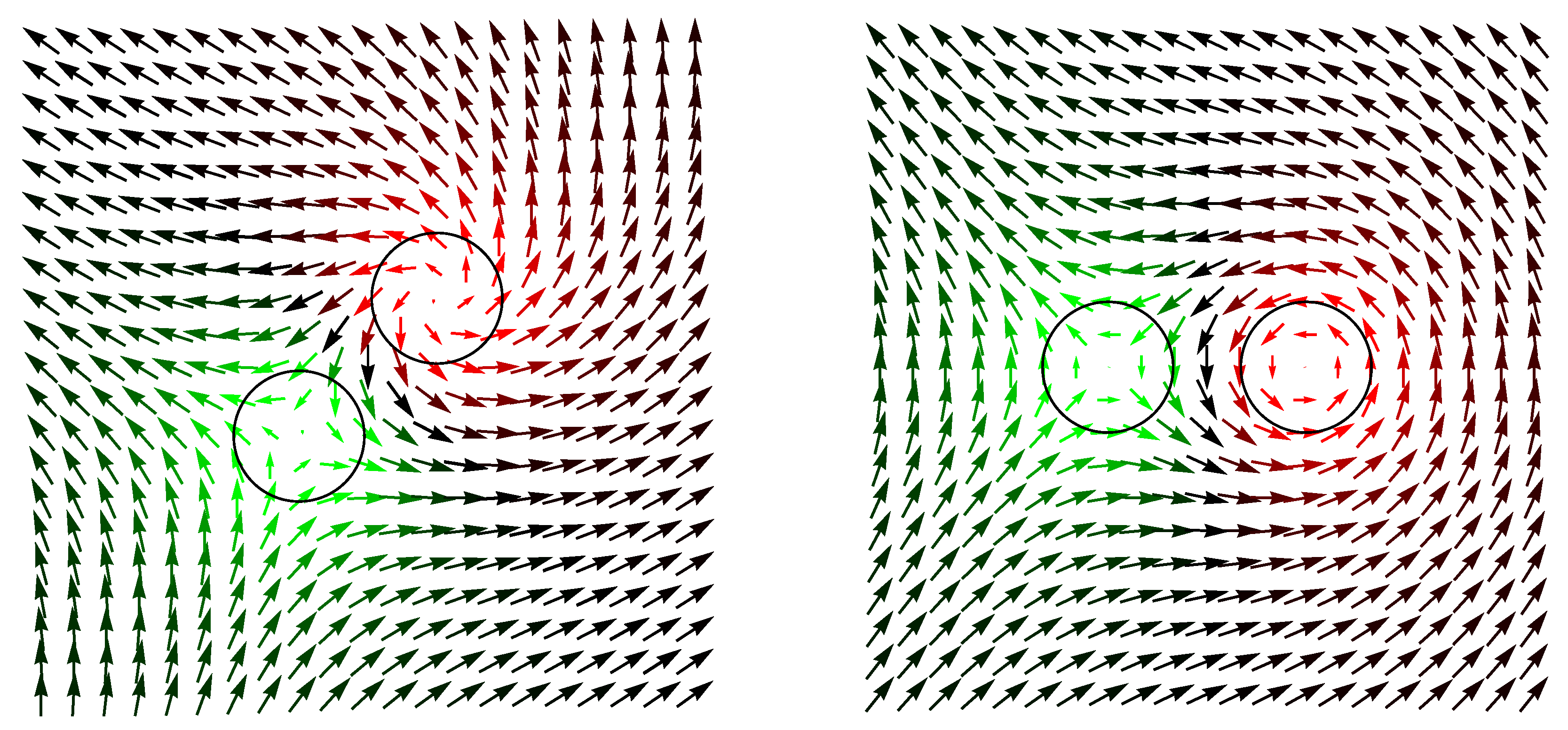
 n -field at given time t to identify the position of solitons. Since these singularities have no chirality there are only two types of singularities, sources (particles) and sinks (antiparticles) of the n -field, with different charge number Z = ± 1 and with singularities from the homotopy class n ( r ) = Z r r .

5.1. Comparison to Maxwell Equations

The singular lines of the sources are related to the properties of the connection and the curvature field
Γ μ ( x ) = ( 59 ) ( 5 ) n ( x ) × μ n ( x ) ,
R μ ν ( x ) = ( 60 ) ( 12 ) μ n ( x ) × ν n ( x ) .
The modulus R μ ν : = R μ ν n defines a dual abelian field strength tensor which reads in SI units
f μ ν = : e 0 4 π ε 0 c 0 R μ ν n = ( 61 ) e 0 4 π ε 0 c 0 n ( μ n × ν n )
In this limit the Lagrange density reduces to
L ED = ( 19 ) α f c 0 4 π 1 4 ( n R μ ν ) ( n R μ ν ) = ( 62 ) 1 4 μ 0 f μ ν ( x ) f μ ν ( x ) .
Up to the sign it has the same form as the Lagrangian of Maxwell’s electrodynamics. In order to compare the dynamics resulting from this Lagrangian to Maxwell equations we relate the world-lines of the singularities with the properties of the n -field. The singularities are located in infinitesimal space-like three dimensional volumes, the centers of hedgehog configurations of the n -field. We describe them by N time-like world-lines of singularities
X i μ ( τ ) i = 1 , , N ,
evolving in time with velocities smaller than c 0 from t = to t = + , or meeting with lines of opposite charge, where particle pairs are created or annihilated. This allows to define for each n -field configuration a singular vector current along the above world-lines
i = 1 N Z i d τ d X i κ ( τ ) d τ δ 4 ( x X i ( τ ) ) : = 1 8 π ε κ λ μ ν λ { n ( μ n × ν n ) } .
For a single soliton resting at the origin with Z = 1 , τ = t , X κ ( τ ) = c 0 t δ 0 κ both sides reduce to a three-dimensional delta-function at the origin δ 3 ( x ) δ 0 κ for the time-component of the singular vector current. Multiplying with e 0 c we get the current density j κ of point-like charges e 0 Z . A further multiplication by μ 0 leads to
μ 0 j κ = ( 65 ) λ e 0 c 0 μ 0 4 π 1 2 ϵ κ λ μ ν n [ μ n × ν n ] f κ λ = ( 62 ) λ f λ κ
and therefore to the inhomogeneous Maxwell equations
μ f μ ν = μ 0 j ν E = ρ ε 0 , 1 μ 0 × B ε 0 t E = j .
These equations are a result of the separation of the soliton field Q ( x ) in singular point-like charges and the surrounding n -field describing electromagnetic fields.
The second set of equation follows from the general equations of motion (53)
0 = ( 53 ) μ [ Γ ν × R μ ν ] = ( 60 ) μ [ ( n × ν n ) × ( μ n × ν n ) ] = = μ { ν n [ n ( μ n × ν n ) ] } = ν n μ [ n ( μ n × ν n ) ] .
This is a condition for magnetic currents
g ν : = e 0 4 π ε 0 μ [ n ( μ n × ν n ) ] = ( 62 ) c 0 μ f μ ν ρ mag = B , g = × E t B .
We conclude, that in this dual formulation we have soft Dirac monopoles and conserved magnetic currents
ν g ν = ( 69 ) 0
which are not quantised. Since n has only two dofs there are only two independent equations in Equation (68). Extending ν n by appropriate factors to the dual field strength tensor we get the equations
f μ ν g ν = ( 69 ) ( 68 ) 0 B g = 0 , c 0 2 B ρ mag = g × E .
The spatial components of these equations we read as dual transformations of a vanishing Lorentz force on magnetic currents. The appearance of these currents is a consequence of the topological restrictions to the n -field. This is the price we have to pay for the quantisation of electric charges on a classical basis. Solutions of the (linear) Maxwell equations are also solutions of the equations of motion (67) and (71). But the two dofs of the n -field are not sufficient to fulfill the homogeneous Maxwell equations exactly and lead to small deviations, to small non-linearities, to magnetic currents. These deviations should remain small for field configurations of minimal energy, which have to respect the topological restrictions and the boundary conditions. It will be interesting to investigate whether the prediction of these magnetic currents is in contradiction to experimental observations. We will see that these magnetic currents do not lead to additional forces acting on electric currents besides the well known Coulomb and Lorentz forces from electric and magnetic field strengths.

5.2. Coulomb and Lorentz Forces

Due to the joint description of charges and electromagnetic fields by Q ( x ) , the interaction of solitons is a consequence of topology [30]. The forces between charges and electromagnetic fields are internal forces and the total force density is vanishing, see Equation (58). The electrodynamic limit provides the possibility to separate charges and their fields.
In the electrodynamic limit the energy-momentum tensor (56) tends to
Θ ν μ ( x ) T ν μ ( x ) = ( 56 ) 1 μ 0 f ν σ ( x ) f μ σ ( x ) L ED ( x ) δ ν μ ,
with components of the same form as the symmetrised energy-momentum tensor in Maxwell’s theory
T 0 0 = H = ( 72 ) ε 0 2 E 2 + c 0 2 B 2 ,
T i 0 = ( 72 ) c ε 0 ( E × B ) i ,
T j i = ( 72 ) ε 0 E i E j + c 0 2 B i B j δ j i 2 ( E 2 + c 0 2 B 2 ) .
We can use Newton’s third axiom where the reaction to the force density of electromagnetic fields is the force density f e μ on charges. Then charges appear as external sources
f e μ : = ( 58 ) ν T ν μ = ( 72 ) 1 μ 0 ν f ν ρ f μ ρ 1 4 μ 0 μ ( f ρ ν f ρ ν ) = = 1 μ 0 [ ν f ν ρ 1 c 0 g ρ f μ ρ + f ν ρ ν f μ ρ f ν ρ ρ f μ ν + 1 2 f ν ρ μ f ρ ν ] = = ( 69 ) 1 μ 0 c 0 f μ ρ g ρ 0 + 1 2 μ 0 f ν ρ [ ν f μ ρ + ρ f ν μ + μ f ρ ν μ 0 ϵ μ ν ρ σ j σ ] = = ( 71 ) ( 67 ) 1 2 ϵ μ ν ρ σ f ν ρ j σ = f μ σ j σ .
The components of the force density on charges read
f e 0 = 1 c 0 j E ,
f e = ρ E + j × B .
Equation (77) describes the loss of power density of the field and the corresponding increase for charges. The spatial force density (78) includes Coulomb- and Lorentz forces acting on point-like electric charges.
The above relations show that the electrodynamic limit of the soliton model corresponds to Maxwell’s electrodynamics (MEdyn), with the distinction that only integer multiples of the electric charge unit are allowed. This restriction leads to the appearance of magnetic currents which do not directly contribute to the forces on electric currents and thus are only internal currents. They are not quantized and influence electric charges only via their electric and magnetic fields.
From MEdyn we know that conserved electric currents are related to a U(1)-gauge invariance.

5.3. U(1) Gauge Invariance

According to Equation (61), R μ ν is a vector in the SU(2) algebra, parallel to n . This gives rise to the emergence of a local U(1) gauge symmetry. A gauge transformation corresponds to a x-dependent rotation of the three basis vectors σ i of the SU(2) algebra under rotations ω ( x ) = ω ( x ) n around n by an arbitrary angle ω ( x )
σ σ ( ω ( x ) ) : = e ω ( x ) n × σ .
For infinitesimal coordinate shifts these transformations read
σ ( ω ( x + d x ) ) = ( 79 ) e d x μ μ ω n × σ ( ω ( x ) ) .
They have to be compensated by an additional rotation of n vectors. The affine connection (4) is the rotational angle transforming n ( x ) to n ( x + d x )
n ( x + d x ) = ( 4 ) e d x μ Γ μ × n ( x ) = n ( x ) + d x μ Γ μ × n , n ( x + d x ) = n ( x ) + d x μ μ n .
Comparing the two equations, we see that Γ μ has to respect
Γ μ × n = ( 81 ) μ n .
Equation (60) satisfies this condition. But Γ μ is fixed by Equation (82) up to a component parallel to n only. This freedom offers the possibility to compensate the basis transformation (80) by the shift
Γ μ = ( 60 ) n × μ n Γ μ : = n × μ n + μ ω n .
With this transformation, algebra valued fields get invariant under basis transformations.
As Equation (83) reminds us the affine connection is not a tensor.
According to the above derivation, the n -field and therefore the coordinates (61) of the curvature tensor R μ ν are invariant under local gauge transformations, realized in this model as basis transformations in the tangential space of S 2 . This S 2 is the parameter space of the soliton field Q ( x ) in the electrodynamic limit (59).
A further important application of the electrodynamic limit is the sector where only electromagnetic waves are present.

5.4. Goldstone Bosons

The minimum q 0 = 0 of the potential in the Lagrangian (19) is degenerate at a two-dimensional manifold. Thus, the vacuum has broken symmetry and the model has two types of Goldstone bosons. The Lagrangian reduces to the form (63). Up to the different sign, this Lagrangian is formally identical to the Lagrangian of Maxwell’s electrodynamics with 2*4 physical dofs of the wave-field in radiation gauge when the time component and the longitudinal component of the gauge field are removed. In distinction, in the present model, the n -field has two dofs only. We describe them by two spherical angles θ ( x ) and ϕ ( x ) . In the electrodynamic limit and in the absence of singularities of the n -field there are no charged particles present and we can assume that the field at spatial infinity “” is independent of the direction. The vacuum has broken symmetry. As a consequence of the Hobart-Derrick theorem [18,19], pure regular n -field configurations moving with velocities smaller than the velocity of light c 0 are unstable. For velocities c 0 they have constant action in time and one can try to describe electromagnetic waves [31]. Due to the isomorphism R 3 S 3 and the topological relation π 3 ( S 2 ) = Z there is an additional quantum number for the n -field, the Hopf number or Gauß linking number v of fibres F defined by n F = const, thus by certain values θ F and ϕ F . Fibers are in general closed lines and for different fibers C 1 and C 2 we can determine a linking number v by the famous double integral of Carl Friedrich Gauß
v = 1 4 π C 1 C 2 r 1 r 2 | r 1 r 2 | 3 · ( d r 1 × d r 2 ) ,
With v = ± 1 we identify right and left polarised photons. v can be modified by the interaction of photons with solitons. The physical equivalent of v is the number of photons n γ in a field configuration.
As described in Refs. [32,33] v can be computed also by one-dimensional integrals from the behavior of neighboring fibers. In such a determination enters the geometry of S 2 in an interesting way.
Crossing solitons in arbitrary direction rotates the spatial Dreibein by 2 π with left or right chirality as depicted in Table 1. Scattering, emission, and absorption processes of photons by solitons are able to modify the chiralities of both types of particles. These geometrical processes need detailed investigations.
Much work on S 2 -fields with different Lagrangians has already been done by Ferreira et al., see e.g., [34] and references therein. A recent article about the closely related field of Topological photonics is [35].

6. Open Questions and Conjectures

In this section, we discuss some features of the model which need future detailed investigations or where, at the moment, we can rely on speculations only.

6.1. Running of the Coupling

The usual conclusion from high-energy scattering experiments is that electrons are point-like. This could counteract this model, since this model suggests a finite size of static electrons of the order of the classical electron radius r cl .
In order to learn from experiments about the property of electrons at distances of r cl and smaller we need high energies. A characteristic relation between radius and energy is c 0 200 MeV fm . 200 MeV electrons are sensible at distances of fm, the 100 GeV electrons of LEP up to distances of 2 attometers.
The solitons of this model are relativistically covariant. A moving soliton is Lorentz compressed. At LEP, electrons reached a γ factor of 2 × 10 5 and therefore could approach another electron in a head-on collision up to distances of 0.5 × 10 5 r cl = 0.014 am. The analogous behavior one can study in the analytical two-particle solutions of the Sine-Gordon model. For γ to infinity, the distance of the closest approach of two solitons approaches zero.
The finite size of solitons of this model leads to a modification of Coulomb’s law at distances of the order of the soliton radius. This effect is known in quantum field theories as running of the coupling. The result of the perturbative calculations in QED is the Uehling potential [36]. It predicts a strong rise of the effective charge of electrons at the order of a few fm. Since nothing in nature seems to be infinitely large or infinitely small, one can see this rise as an indication for an effective size of electrons at this order of magnitude.
The model discussed in this article gets a running of the coupling at the classical level. In due course, we will publish a paper about this effect. The numerical calculations were prepared in a paper published recently in Few-Body systems [28].

6.2. Orthogonality of E and B

We have seen in Equation (44) that the conservation of topological charge leads to E B = 0 . In the electrodynamic limit we have R μ ν = ( 62 ) R μ ν n and therefore also E · B = 0 , as is also implied by Equation (71) for non-vanishing magnetic currents. This seems to contradict the experimental situation, where we have no problems producing parallel electric and magnetic fields. There is possibly a way out of this problem, see also the discussion in Ref. [29]. In the electrodynamic limit, the basic field is the unit-vector field n ( x ) . A constant n -field corresponds to zero-field strength. One can get the electric field by an n -field rotating in space. Due to the topological restriction, a homogeneous electric field can be produced only in a finite spatial region. The solution, given in Ref. [29] looks more complicated than in Maxwell’s theory, but it agrees better to the experimental situation with capacitor plates of finite size and finite charge and fields whose homogeneity is only approximate. Magnetic fields originate from non-vanishing time components of the connection and thus from the rotations of n -vectors in time. Electric currents in a wire, the source of magnetic fields, correspond to hoppings of electrons from one ion to the next in a very short time, a strong time-dependence of n -fields is necessary to produce a reasonable magnetic field.
The orthogonality of E and B follows from the interpretation of the field strength as the curvature of the unit vector field n , see Equation (61). It is not derived from the Lagrangian and thus not a consequence of the dynamics. It is valid at the level of distances between elementary charges. This leads to the idea, that the orthogonality is present on a microscopic level and parallelity may be achieved on a macroscopic time-averaged level.

6.3. Quantum Effects

The model formulated in Section 2 is a classical model. For around 100 years, we have known that nature in atomic and subatomic physics is dominated by quantum effects. Under the present paradigm of the quantum field theory, one would include quantum effects by integrations over all possible quantum fluctuations. In Ref. [37] it was shown that such integrations lead to diverging integrals. In distinction to Maxwell’s electrodynamics (MEdyn) the presented model is from the beginning finite. Therefore, there seems no need for regularization and renormalization. If the model is of some applicability, there must be another method to include quantum fluctuations and interference, encoded in the path integral formulation of quantum mechanics and quantum field theory by its complex Boltzmann factor e i S , where S is the action attributed to field configurations. There is some freedom to achieve this goal since nobody knows how nature does, in order to produce the effects which are perfectly described by quantum mechanics.
There are hundreds of books and thousands of articles about the riddles and the philosophical implications of quantum mechanics, but there are only a few ideas suggesting mechanisms. I know of only one experiment which may give an idea for a mechanism. This is Couder’s experiment [10] of bouncing oil drops which, as I think, supports De Broglie’s idea [38] of pilot waves. The bouncing drops are interacting with waves and produce waves themselves [15]. In the critical double-slit experiments, the waves pass both slits, whereas every particle passes only one slit. The particle trajectories are influenced by the interfering waves and lead to an interference pattern at the detectors.
Can we find such a mechanism in our model? Quantum mechanical fluctuations are action fluctuations and not energy fluctuations. This could mean, the energy is transferred for a short moment and then again subtracted. Some types of waves, unknown in MEdyn, passing a particle could possibly provide such a phenomenon.
There are two types of fields in our model which are unknown in MEdyn, magnetic currents g μ and waves in the angular parameter α of the Q-field
Q = ( 1 ) q 0 i q σ = ( 3 ) cos α i σ n sin α .
α is related to the rotational angle ω of Dreibeins in space by ω = 2 α . Magnetic currents are non-vanishing sources of magnetic fields [29]. As was discussed in Section 5.2 magnetic currents do not contribute to Coulomb and Lorentz forces, see Equation (78) and therefore do not directly influence the motion of charged particles. The appearance of magnetic currents is a result of the non-Abelian nature of the soliton field. Due to the topological restrictions, electromagnetic waves may be accompanied by magnetic currents, which in the vacuum propagate with the velocity of light in the direction given by the Poynting vector. The magnetic currents coming from the soliton description are different from the Dirac magnetic currents because they are not quantized and cannot be associated with massive magnetic charges. They are suppressed by the request of minimal energy and seem rather tiny deviations from the solutions of the homogeneous Maxwell equations, in case these can not be fulfilled due to the topological restrictions of the n -field. Since magnetic currents seem not to have measurable consequences, they should be ruled out as guiding waves.
α -
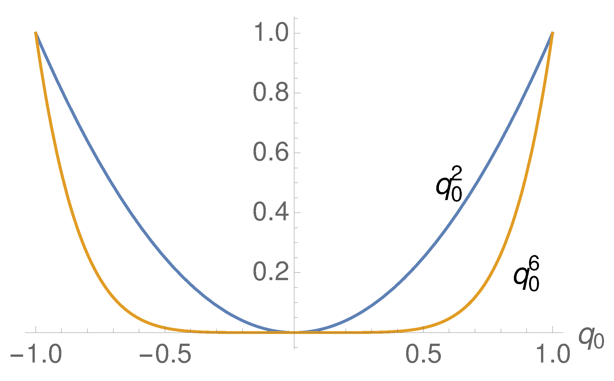
waves are governed by the shape of the potential term L pot in the Lagrangian (19) with its unusual power q 0 6 , see Figure 6. In Ref. [37] it was shown that a q 0 2 dependence of the potential term would lead to vibrational excitations of solitons. The aim to compare solitons with the lightest charged fermions is to rule out such excitations. Higher even powers in q 0 do not show such vibrations but allow for waves in q 0 = cos α . For radial waves a Schrödinger-type equation
1 2 Δ + V ( r ) η k ( r ) = ω k 2 η k ( r ) .
with the potential
V ( r ) = 1 + 3 cos 2 α 4 r 2 + 15 r 2 2 r 0 4 cos 4 α = ( 32 ) 2 r 0 4 + r 0 2 r 2 + 14 r 4 2 r 0 2 r 2 ( r 0 2 + r 2 ) 2
was derived which is repulsive everywhere and has no bound states. The spectrum of spherical waves
η k = e ± i k r r with ω k 2 = 1 2 k 2 .
is continuous.
In scattering processes between photons lumps of non-vanishing q 0 ( x ) = ( 3 ) cos α are produced. As mentioned in Section 5.4 photons are characterized by a field of purely imaginary unit quaternions, see Equation (59). In scattering processes two such fields Q 1 ( x ) and Q 2 ( x ) have to be multiplied
Q 1 ( x ) Q 2 ( x ) = [ i σ n 1 ( x ) ] [ i σ n 2 ( x ) ] = ( n 1 n 2 ) i σ ( n 1 × n 2 )
leading to a non-vanishing real part cos α = n 1 n 2 and therefore to a small contribution to the potential energy, to a tiny massive lump acting like a small particle.
An oscillation of non-vanishing q 0 in some direction n o could bounce way and back in the flat region of the q 0 6 -potential. If such an oscillation approaches a soliton, due to its tiny mass contributions it should shift the soliton center depending on the angle between n o and the solitons n -vector in this spatial region. Due to the above-mentioned oscillation in the q 0 6 -potential the soliton center should move alternating in forward and backward direction, i.e., adding and subtracting energy and momentum in short sequence. This would maintain energy and momentum constant, but increase the action. It will be interesting to investigate in more detail whether such α -waves could provide a model for the physical nature of a guiding field. In diffraction experiments, the diffracted field would exist independent of the presence of solitons and the solitons could maintain their corpuscular nature all along with the experiment as the authors of Ref. [39] expect for the zero-point fluctuations as guiding field.
α -waves could be a candidate for dark matter. Most of the community is looking for dark particles. Up to now, nobody has found dark particles. I think, dark matter escapes our detectors since it does not have the form of particles and it does not modify the kinetic energy of particles. α -waves do not have particle structure. Due to their contribution to the potential, they are rather tiny lumps of not quantized mass.

6.4. A Possible Mechanism of Cosmic Inflation

Some cosmological models assume an inflationary epoch [40] in the early universe, a very short period of exponential expansion of the cosmos, explaining the large-scale structures of our universe, its flatness, and the relative homogeneity and isotropy of the cosmic microwave background. Our model provides a possible mechanism for inflation. A transition from an initial field configuration in the early universe from an initial stationary state with positive energy density H before
Q ( x ) 1 Λ = ( 19 ) 1 r 0 4 H before : = L pot before = ( 19 ) α f c 0 4 π r 0 4
to a stable vacuum with vanishing energy density H after
Q ( x ) i σ 3 Λ = ( 19 ) 0 H after : = L pot after = ( 19 ) 0
after inflation. This transition would have released the energy density
H before H after = ( 91 ) ( 90 ) = α f c 0 4 π r 0 4 = ( 35 ) 4.8 keV / fm 3 = 7.7 × 10 29 J / m 3 .
Despite the vanishing energy-momentum tensor in the absence of solitons, see Equation (91), there is a running of the coupling due to the modification of Coulomb’s law at distances of the order of the soliton radius, as will be discussed in detail in a forthcoming article. This is in contradistinction to quantum electrodynamics, where quantum corrections lead to a running coupling described by a non-vanishing beta-function. There, due to the proportionality between beta-function and the value of the trace of the energy-momentum tensor, see Eq. (19.157) of Peskin-Schröder [36], a vanishing trace would prevent the running of the coupling.

6.5. Cosmological Constant

1917 Einstein has introduced a cosmological constant in general relativity to compensate for the attractive interaction of the mass density and to get stationary solutions of the field equations. In cosmological models, like the Λ CDM model [41], the cosmological constant is related to an energy density of the vacuum explaining the observed cosmic expansion. The Planck collaboration gives in its 2018 results [42] a cosmological energy density of 0.69 ρ crit , where the critical energy density is 4.9 GeV m 3 .
The potential term L pot in the Lagrangian (19) acts as a cosmological function, contributing to the energy density of the universe. Due to the application of the Hobart-Derrick theorem a quarter of the rest energy of solitons is contributed from the potential energy H pot , see Equation (23). If this ratio would also be valid for nucleons an average density of nucleons of 14.5 nucleons per m 3 would agree with the measured energy density. In comparison, the prediction of field theory deviates many orders of magnitude—a still unsolved problem.
As discussed in Section 6.3, due to their contributions to the potential energy α -waves would also participate in the cosmological constant, the average of the cosmological function.

7. Conclusions

7.1. Comparison to Other Models

The model discussed in this article has many features in common with other well-known models. The Lagrangian defined in Equation (19) can be seen as a generalization of the Sine-Gordon model [6], a model in 1+1D with one field degree of freedom (dof), generalized to a field in 3+1D with three dofs.
Up to the difference between the groups, SU(2) and SO(3) the dofs are the same as those of the Skyrme model [16,17]. The difference is in the terms compressing solitons, in the Skyrme model the compressing term has two derivatives, in the Lagrangian (19) it is substituted by the term L pot without derivatives.
Dirac [20,21] suggested introducing magnetic monopoles in Maxwell’s electrodynamics (MEdyn) by defining a line-like singularity, the well-known Dirac string. Wu and Yang [22,23] succeeded in removing this singular line using a normalized three-component scalar field n to describe the field of monopoles, but they did not remove the singularity in the center of the monopoles.
’T Hooft [43] and Polyakov [44] investigated monopoles in gauge field theories and identified monopoles in the Georgi-Glashow model. This model has a triplet of gauge fields with 3 × 4 dofs and a triplet of scalar (Higgs) fields, in summary, 15 dofs. The energy of these monopoles was estimated with the order of the mass of the W-boson multiplied with the inverse of Sommerfeld’s fine structure constant. As was shown in [45,46,47] in the so-called BPS-limit [48,49] of the massless Higgs boson, monopoles and antimonopoles keep interacting with each other Coulomb-like. However, the force between two monopoles or two antimonopoles vanishes, whereas the interaction strength between a monopole and an antimonopole doubles in comparison with the limit where the Higgs boson is much heavier than the W-bosons of the 3D Georgi-Glashow model.
An attempt to construct the Standard Model with Monopoles was undertaken by Vachaspati [50]. However, in that article, which is aimed at discussing the algebraic properties of possible mappings between particles and monopoles, dynamical features were set aside.
We describe particles and their fields with the same dofs, in analogy to the Sine-Gordon and the Skyrme model. Only three dofs of an SO(3)-field are necessary to describe charges and their fields. Since these three dofs can be interpreted as orientations of spatial Dreibeins we can ascribe these properties to space-time. In this way, we would succeed to describe the two long-range interactions, electrodynamics, and gravitation, by the properties of space-time only.
An important test of the applicability of this model is an investigation of the differences to MEdyn.

7.2. Comparison to Maxwell’s Electrodynamics

The model describes charges with long-range forces as we have in Maxwell’s electrodynamics (MEdyn). As already mentioned, this model can not substitute Maxwell’s electrodynamics and the SM. The purpose of this chapter is to try to enumerate where this model differs from these theories, where it may be successful, and where it may fail.
Particles are characterized by topological quantum numbers, only artificially they can be separated from their fields. Such separation leads to the well-known singularities of point-like charges.
The following properties agree with MEdyn:
  • The Lagrangian (19) is Lorentz covariant, thus the laws of special relativity are respected.
  • Charges have Coulombic fields fulfilling Gaußes law (67).
  • Charges interact via 1 r 2 electric fields (27), they feel Coulomb and Lorentz forces, see Section 5.2.
  • A local U(1) gauge invariance is respected, see Section 5.3.
  • There are two dofs of massless excitations for photons, see Section 5.4.
The critical questions concern the differences to MEdyn. Several differences agree with the experiment, others have to be investigated in detail, whether they differ only superficially or concern deep discrepancies. In distinction to MEdyn we find the following properties:
  • Electric charges are quantized, see Section 3.2.1, like the magnetic charges of Dirac monopoles. The charge is a topological quantum number.
  • The topological construction explains the astonishing mirror properties of particles and antiparticles [5], see Section 3.2.
  • The mass of solitons is completely due to field energy, see Equation (29), and finite.
  • The self-energy of charges is finite and does not need regularisation and renormalization, see Equation (34).
  • Charges and their fields are described by the same dofs, see Section 2, by SO(3) rotational degrees of freedom. The calculations are simplified using the dofs, see Equation (1), of the double covering group SU(2) of SO(3).
  • These SO(3) dofs can be interpreted as orientations of spatial Dreibeins, see Section 2. Thus, besides the properties of space-time, no additional fields are necessary to describe electromagnetism and gravitation.
  • Gauge symmetry is explained as a geometrical phenomenon, as basis changes in the tangential manifold on S 3 , see the paragraph between Equations (13) and (15).
  • Spin appears with usual quantization properties known from quantum mechanics, see Section 3.2.3, and respects the combination rules of representations of SU(2). Spin is attributed to field configurations with values in the group manifold, whereas in quantum field theories it is usually attributed to algebra-valued fields acting on vectors in the corresponding representation.
  • There are four basic configurations of solitons, see Table 1, with the quantum numbers (45) of components of Dirac spinors.
  • Solitons and antisolitons have opposite internal parity, see Table 1, as is well-known for the description of electrons and positrons with the Dirac equation.
  • Solitons are characterized by a chirality quantum number which can be related to the sign of the magnetic quantum number.
  • Spin contributes to angular momentum due to internal rotations of soliton centers, see Figure 5.
  • The canonical energy-momentum tensor (56) does not need additional symmetrization. It is automatically symmetric.
  • Due to the dual representation (15) of the field strength tensor static charges are described by the spatial components of vector fields (25). For time-dependent phenomena, like moving charges, electric currents and magnetic fields, non-vanishing time components of the connection Γ μ are necessary, see Equations (12) and (15).
  • The finite size of solitons leads to a modification of the Coulomb’s law at distances of the order of the soliton radius [28]. This effect is known in quantum field theories as running of the coupling, see Section 6.1.
  • The local U(1) gauge invariance is explained by the free choice of the bases in the tangential spaces of the S 2 manifold, see Section 5.3.
  • Photons are characterized by a topological quantum number, the Gaußian linking number (84) of fibers of the S 2 -field, the soliton field in the electrodynamic limit.
  • The photon number can be modified by interaction of photons with charges, see Section 5.4.
The following properties differing from MEdyn need deeper investigation and may possibly differ from experiments with electrons and photons.
  • Spin and magnetic moment are dynamical properties. They are consequences of movements of solitons or time-dependent field variations in their surroundings.
  • Electric and magnetic field vectors are perpendicular to each other, see Section 6.2. This is in obvious contradiction to experimental realizations of parallel electric and magnetic fields. An excuse may be, that this property may be realized on a microscopic level and allows for parallelity of these fields on a macroscopic level.
  • The existence of unquantized magnetic currents is allowed. These currents do not directly appear in Lorentz forces. They contribute only via their magnetic fields.
  • α -waves with oscillating values of q 0 = cos α feel non-vanishing values of the potential energy density and contribute therefore to matter density. Such non-topological excitations were not directly detected. If they exist, they contribute to dark matter, see Section 6.3.
  • α -waves lead to additional forces on particles and are a possible origin of quantum fluctuations.
  • The potential term allows for a mechanism of cosmic inflation.
  • The potential term contributes to dark energy.
This model tries to give an idea about a possible direction of future investigations. One should not assume that it can provide a final answer to all questions which are left open by quantum theory and quantum field theory. Both theories have a tremendous success. It is obvious that the model cannot compete with their excellent and precise predictions and the century-long efforts of numerous scientists to describe the properties of nature in the most fundamental domain. But this does not mean that one should not think about scenarios that finally could lead to a deeper understanding of the mechanisms in nature. This could allow us to answer some questions, left open by quantum mechanics and quantum field theory. It could help to answer how nature works to produce the interesting riddles which we could not solve yet.
Some of the questions posed by this model concerning electrodynamics, quantum theory, and quantum field theory are enumerated in the section with critical remarks. Many may still be missing. Essential open problems are also those related to the three other fundamental forces, gravitational, strong, and weak interactions.
If an extension of this model is of some relevance for describing the properties of nature, one could summarise its philosophy in: Particles are properties of regions of space, characterized by topological quantum numbers. Therefore I would like to call it: “Model of topological particles”.

8. Aftermath

In its fundaments, physics is measurements of distances of objects and times of events, and an explanation of their relations.
This may indicate, that
Physics is geometry and not algebra.
Finally, one should use algebra to describe the geometry.
General Relativity:
Wheeler: “Spacetime tells matter how to move;
matter tells spacetime how to curve”. [51]
My addition for Electrodynamics:
⋯ Charges and electromagnetic fields tell space how to rotate.

Funding

This research received no external funding.

Acknowledgments

I want to thank Jarek Duda for his interest in the model and his support to make it more public in the community. To the anonymous referees of this manuscript, I am grateful for their constructive comments.

Conflicts of Interest

The authors declare no conflict of interest.

Note

1
With bold characters we indicate vectors in 3D.

References

  1. Odom, B.; Hanneke, D.; D’Urso, B.; Gabrielse, G. New Measurement of the Electron Magnetic Moment Using a One-Electron Quantum Cyclotron. Phys. Rev. Lett. 2006, 97, 030801. [Google Scholar] [CrossRef] [PubMed] [Green Version]
  2. Bohm, D. David Bohm’s Critique of Modern Physics: Letters to Jeffrey Bub, 1966–1969; Springer: Cham, Switzerland, 2020. [Google Scholar]
  3. Smolin, L. The Trouble with Physics: The Rise of String Theory, the Fall of a Science, and What Comes Next; Houghton Mifflin: Boston, MA, USA, 2006. [Google Scholar]
  4. Woit, P. Not Even Wrong: The Failure of String Theory and the Search for Unity in Physical Law; Basic Books: New York, NY, USA, 2006. [Google Scholar]
  5. Borchert, M.J.; Devlin, J.A.; AU Erlewein, S.R.; Fleck, M.; Harrington, J.A.; Higuchi, T.; Latacz, B.M.; Voelksen, F.; Wursten, E.J.; Abbass, F.; et al. A 16-parts-per-trillion measurement of the antiproton-to-proton charge–mass ratio. Nature 2022, 601, 53–57. [Google Scholar] [CrossRef] [PubMed]
  6. Remoissenet, M. Waves Called Solitons: Concepts and Experiments; Advanced Texts in Physics; Springer: New York, NY, USA, 2003. [Google Scholar]
  7. Pietschmann, H. Consequences of Minkowskis Unification of Space and Time for a Philosophy of Nature. In Minkowski Spacetime: A Hundred Years Later; Petkov, V., Ed.; Springer: Dordrecht, The Netherlands, 2010; pp. 319–326. [Google Scholar] [CrossRef] [Green Version]
  8. Cabaret, D.M.; Grandou, T.; Grange, G.M.; Perrier, E. Elementary Particles: What are they? Substances, elements and primary matter. arXiv 2021, arXiv:2103.05522. [Google Scholar]
  9. Cabaret, D.M.; Grandou, T.; Perrier, E. Status of the wave function of Quantum Mechanics, or, What is Quantum Mechanics trying to tell us? arXiv 2021, arXiv:2103.05504. [Google Scholar]
  10. Couder, Y.; Fort, E.; Gautier, C.H.; Boudaoud, A. From Bouncing to Floating: Noncoalescence of Drops on a Fluid Bath. Phys. Rev. Lett. 2005, 94, 177801. [Google Scholar] [CrossRef] [PubMed] [Green Version]
  11. Anderson, P.W. More Is Different: Broken symmetry and the nature of the hierarchical structure of science. Science 1972, 177, 393–396. [Google Scholar] [CrossRef] [Green Version]
  12. Hooft, G. Past and Future of Gauge Theory. In One Hundred Years of Gauge Theory; Past, Present and Future Perspectives; Fundamental Theories of Physics; De Bianchi, S., Kiefer, C., Eds.; Springer International Publishing: New Yrok, NY, USA, 2020; Volume 199, pp. 301–313. [Google Scholar]
  13. Faber, M. A Model for topological fermions. Few Body Syst. 2001, 30, 149–186, arXiv:9910221. [Google Scholar] [CrossRef] [Green Version]
  14. Kouneiher, J. Conceptual Foundations of Soliton Versus Particle Dualities Toward a Topological Model for Matter. Int. J. Theor. Phys. 2016, 55, 2949–2968. [Google Scholar] [CrossRef]
  15. Bush, J.W. Pilot-Wave Hydrodynamics. Annu. Rev. Fluid Mech. 2015, 47, 269–292. [Google Scholar] [CrossRef] [Green Version]
  16. Skyrme, T.H.R. A Nonlinear theory of strong interactions. Proc. R. Soc. Lond. A 1958, 247, 260–278. [Google Scholar] [CrossRef]
  17. Skyrme, T.H.R. A Nonlinear field theory. Proc. R. Soc. Lond. A 1961, 260, 127–138. [Google Scholar] [CrossRef]
  18. Hobart, R. On the Instability of a Class of Unitary Field Models. Proc. Phys. Soc. Lond. 1963, 82, 201–203. [Google Scholar] [CrossRef]
  19. Derrick, G. Comments on Nonlinear Wave Equations as Models for Elementary Particles. J. Math. Phys. 1964, 5, 1252–1254. [Google Scholar] [CrossRef] [Green Version]
  20. Dirac, P.A.M. Quantised singularities in the electromagnetic field. Proc. Roy. Soc. Lond. 1931, A133, 60–72. [Google Scholar]
  21. Dirac, P.A.M. The Theory of magnetic poles. Phys. Rev. 1948, 74, 817–830. [Google Scholar] [CrossRef]
  22. Wu, T.T.; Yang, C.N. Some remarks about unquantized nonabelian gauge fields. Phys. Rev. 1975, D12, 3843–3844. [Google Scholar]
  23. Wu, T.T.; Yang, C.N. Dirac’s Monopole Without Strings: Classical Lagrangian Theory. Phys. Rev. 1976, D14, 437–445. [Google Scholar] [CrossRef]
  24. Wabnig, J. Interaction in the Model of Topological Fermions. Diploma Thesis, Physics, Technische Universitat Wien, Wien, Austria, 2001. [Google Scholar]
  25. Resch, J. Numerische Analyse an Dipolkonfigurationen im Modell topologischer Fermionen. Diploma Thesis, Physics, Technische Universitat Wien, Wien, Austria, 2011. [Google Scholar]
  26. Theuerkauf, D. Charged Particles in the Model of Topological Fermions. Diploma Thesis, Physics, Technische Universitat Wien, Wien, Austria, 2016. [Google Scholar]
  27. Anmasser, F. Running Coupling Constant in the Model of Topological Fermions. Diploma Thesis, Physics, Technische Universitat Wien, Wien, Austria, 2021. [Google Scholar]
  28. Anmasser, F.; Theuerkauf, D.; Faber, M. About the solution of the numerical instability for topological solitons with long range interaction. Few-Body Syst. 2021, 62, 84, arXiv:2108.07309. [Google Scholar] [CrossRef]
  29. Faber, M.; Kobushkin, A.P. Electrodynamic limit in a model for charged solitons. Phys. Rev. 2004, D69, 116002, arXiv:0207167. [Google Scholar] [CrossRef] [Green Version]
  30. Chan, H.; Tsou, S. Some Elementary Gauge Theory Concepts; World Scientific Lecture Notes in Physics; World Scientific: Singapore, 1993. [Google Scholar]
  31. Borisyuk, D.; Faber, M.; Kobushkin, A. Electro-Magnetic Waves within a Model for Charged Solitons. J. Phys. 2007, A40, 525–531, arXiv:0708.3173. [Google Scholar] [CrossRef] [Green Version]
  32. Jech, M. Die Hopfzahl in einer SU(2)-Feldtheorie. Master’s Thesis, Technische Universitat Wien, Wien, Austria, 2014. [Google Scholar]
  33. Faber, M. Charges and Electromagnetic radiation as topological excitations. Adv. High Energy Phys. 2017, 2017, 9340516, arXiv:1707.03196. [Google Scholar] [CrossRef] [Green Version]
  34. Ferreira, L.; Sawado, N.; Toda, K. Static Hopfions in the extended Skyrme-Faddeev model. J. High Energy Phys. 2009, 2009, 124. [Google Scholar] [CrossRef] [Green Version]
  35. Shen, Y.; Hou, Y.; Papasimakis, N.; Zheludev, N. Supertoroidal light pulses as electromagnetic skyrmions propagating in free space. Nat. Commun. 2021, 12, 5891. [Google Scholar] [CrossRef] [PubMed]
  36. Peskin, M.; Schroeder, D. An Introduction To Quantum Field Theory; Perseus Books Publishing, L.L.C.: New York, NY, USA, 1995; p. 864. [Google Scholar]
  37. Faber, M.; Kobushkin, A.; Pitschmann, M. Shape vibrations of topological fermions. Adv. Stud. Theor. Phys. 2008, 2, 11–22, arXiv:0812.4225. [Google Scholar]
  38. de Broglie, L. La mécanique ondulatoire et la structure atomique de la matière et du rayonnement. Journal de Physique et le Radium 1927, 8, 225–241. [Google Scholar] [CrossRef]
  39. De la Peña, L.; Cetto, A.M.; Valdés-Hernández, A. The Emerging Quantum; Springer International Publishing: New York, NY, USA, 2015; p. 366. [Google Scholar] [CrossRef] [Green Version]
  40. Guth, A.H. Inflationary universe: A possible solution to the horizon and flatness problems. Phys. Rev. D 1981, 23, 347–356. [Google Scholar] [CrossRef] [Green Version]
  41. Turner, M.S. ΛCDM: Much more than we expected, but now less than what we want. arXiv 2021, arXiv:2109.01760. [Google Scholar]
  42. Aghanim, N.; Akrami, Y.; Arroja, F.; Ashdown, M.; Aumont, J.; Baccigalupi, C.; Ballardini, M.; Banday, A.J.; Barreiro, R.B. Planck2018 results. Astron. Astrophys. 2020, 641, A1. [Google Scholar] [CrossRef] [Green Version]
  43. ’t Hooft, G. Magnetic Monopoles in Unified Gauge Theories. Nucl. Phys. B 1974, 79, 276–284. [Google Scholar] [CrossRef] [Green Version]
  44. Polyakov, A.M. Particle Spectrum in Quantum Field Theory. JETP Lett. 1974, 20, 194–195. [Google Scholar]
  45. Polyakov, A.M. Quark Confinement and Topology of Gauge Groups. Nucl. Phys. B 1977, 120, 429–458. [Google Scholar] [CrossRef]
  46. Dietz, K.; Filk, T. Critical Higgs mass for the (2 + 1) dimensional Georgi-Glashow model. Nucl. Phys. B 1980, 164, 536–545. [Google Scholar] [CrossRef]
  47. Manton, N.S. The Force Between ’t Hooft-Polyakov Monopoles. Nucl. Phys. B 1977, 126, 525–541. [Google Scholar] [CrossRef]
  48. Bogomol’nyi, E.B. Stability of classical solutions. Sov. J. Nucl. Phys. 1976, 24, 449. [Google Scholar]
  49. Prasad, M.K.; Sommerfield, C.M. An Exact Classical Solution for the ’t Hooft Monopole and the Julia-Zee Dyon. Phys. Rev. Lett. 1975, 35, 760–762. [Google Scholar] [CrossRef]
  50. Vachaspati, T. An Attempt to construct the Standard Model with monopoles. Phys. Rev. Lett. 1996, 76, 188–191, arXiv:9509271. [Google Scholar] [CrossRef] [Green Version]
  51. Wheeler, J.A.; Ford, K. Geons, Black Holes, and Quantum Foam: A Life in Physics; W.W.Norton & Company: New York, NY, USA, 1998; p. 235. [Google Scholar]
Figure 1. Depicted is the imaginary part q ( x ) = n ( x ) sin α ( x ) of the soliton field Q ( x ) of Equation (1) in a symmetry plane.
Universe 08 00073 g001
Figure 2. Radial energy densities of the stable soliton solution according to Equation (33). The prefactor in h is omitted.
Universe 08 00073 g002
Figure 3. Schematic diagrams for the Q-field (arrows) and the flux lines (lines) of two opposite unit charges, Z = Q el = 0 . The configurations are rotational symmetric around the axis through the two charge centers. The red/green arrows symbolise values of q = n sin α for postive/negative values of q 0 = cos α . For q 0 0 the arrows are getting darker or black. The left configuration belongs to the topological quantum numbers Q = s = 0 and the left one to Q = s = 1 . Observe that field lines connect points of constant n -field.
Universe 08 00073 g003
Figure 4. The rotating inner sphere is connected by an arbitrary number of wires to the outer sphere. Rigid spheres of the increasing radius with fixed piercings rotate around varying axes. The inner sphere performs a 4 π rotation around the axis indicated by the black dot. The red dot shows the status of the positive rotation in the sequence 0 , π , 2 π , 3 π , 4 π . The set of these rotations corresponds to a big circle on S 3 . For spheres from inside to outside, these sets build smaller and smaller circles contracting at the outer sphere to no rotation.
Universe 08 00073 g004
Figure 5. Two schematic diagrams for a rotating dipole which differ by rotations of 45 and 90 from Figure 3b. The imaginary part of the SU(2)-field are indicated by arrows. The visibility of the positions of the two charges is enhanced by surrounding circles. Red/green/black arrows indicate q 0 > 0 / q 0 < 0 / q 0 = 0 .
Universe 08 00073 g005
Figure 6. Observe the flat region of the function q 0 6 .
Universe 08 00073 g006
Table 1. The transformations T of the hedge-hog configuration in the first column, see Equation (24), modify the fields n and q 0 and the topological quantum numbers Z and Q . The diagrams show the imaginary components q = n sin α of the soliton field, in full red for the hemisphere with q 0 > 0 and in dashed green for q 0 < 0 .
T = 1 T = z T = Π n T = z Π n
n = r / r n = r / r n = r / r n = r / r
q 0 0 q 0 0 q 0 0 q 0 0
Z = 1 Z = 1 Z = 1 Z = 1
Q = 1 2 Q = 1 2 Q = 1 2 Q = 1 2
   Universe 08 00073 i001   Universe 08 00073 i002   Universe 08 00073 i003   Universe 08 00073 i004
Publisher’s Note: MDPI stays neutral with regard to jurisdictional claims in published maps and institutional affiliations.

