1. Introduction
The accumulation of observational data in favour of a physical tension between low and high redshift determinations of the Hubble constant indicates potential new physics beyond the standard model [
1,
2,
3]. There are several methods nowadays for the determination of Hubble’s constant. In the process of observational determination of the Hubble tension many mechanisms are involved: the study of the standard candles as probes for luminosity distances, early time calibrations and the sound horizon as a standard ruler, time delays via gravitational lenses, gravitational waves, etc. [
4,
5]. Various methods require several of those tools, and hence errors are bound to accumulate. We have today two particularly accurate and powerful methods for the determination of the
tension. One that relies on the cosmic microwave background, under the assumption of a cold dark matter universe with a cosmological constant
(
CDM) and the other relying on direct measurements from supernovae. These methods were recently highly refined by employing data both from the Planck satellite (for the cosmic microwave background) and from GAIA, a space telescope system providing accurate data for the later method. The Hubble constant inferred from CMB has been calculated to be
km s
Mpc
(Planck) or
(DES+BAO+BBN) [
6] while the supernovae observations insist on a value of
km s
Mpc
(SH0ES collaboration) [
7] with the distinction between the distributions related to the two types of observations being significant up to
combining all data of [
6,
8] and
difference in the prediction of
from Planck cosmic microwave background observations under
, with no indication that the discrepancy arises from measurement uncertainties or analysis variations considered to date. Basically, this leads us to a tension between the “local” and the “global” measurements of the Hubble constant that can only hardly be considered to result from systematic errors or other data-related biases. Indeed, this seems to be a fundamental problem in today’s cosmology and astrophysics, as it involves not only insights on the accuracy of various observational methods, but also a deeper understanding of elementary processes in high energy physics and maybe even quantum gravity [
9].
It is worth mentioning that while such a discrepancy has been observed in previous data, the interest of the cosmology community peaked when the latest, far more accurate, observational results not only re-confirmed the above mentioned tension, but they also made it sharper [
10]. While this observational discrepancy has not been in the focus of theoretical model-builders, there have been at least a few attempts to give explanations based on new physics or modified fundamentals [
11,
12].
Some explanations such as the reduction of the cosmic sound horizon, alone, could not fully resolve this tension [
13]. The reconciliation of the theories with observations is delicate. Neutrinos [
14], axions [
15], or other moduli-particles [
16] have been considered as possible explanations, together with modified dark energy contributions at the early stages of cosmological evolution, thermal effects of the early axions [
12,
17], axions interacting with a Dilaton [
15], or the reduction of the dark matter particles via so called dark matter cannibalism reactions [
18]. These later models correspond to a situation in which three dark matter particles can annihilate into two particles. Such models are particularly important for solving the
tensions because they can increase the dark radiation component in the early universe. This is a strongly exothermic process where the cannibal dark matter behaves as a warm dark matter component for a longer period of time, becoming non-relativistic at later times than the cold dark matter. However, this process strongly suppresses structure growth, being able to account only for around
of the dark matter overall [
19]. In general, warm dark matter would suppress structure formation and hence there is a natural limit as to how high the concentration of warm dark matter could be.
In all cases it was not possible to fully acknowledge the evolution of the Hubble constant as observed presently. In this article, I will provide a new theoretical approach, although still based on axion contributions to the cosmological evolution. While axion solutions have been considered before, no analysis relying on the fundamental origin of axions has been made up to now. Axions indeed are dark matter candidates that appear as an extension to the standard model of elementary particles and are motivated by the strong CP problem. The strong CP problem refers to the unexpected absence of a CP violating term in Quantum Chromodynamics (QCD) albeit not forbidden by any usual restrictions. Given the experimental observations, if such a CP breaking term were to exist, it would appear to be unjustifiably small leading to a hierarchy problem. The solution to this problem is given by the so called Peccei–Quinn mechanism that involves axial degrees of freedom and an additional (Peccei–Quinn) symmetry broken spontaneously, and hence giving rise to the Axion, and further broken explicitly by various instanton-like mechanisms, providing mass to the newly required Axion. As we may notice, while the Axion, and the associated axial degrees of freedom do solve the strong CP problem, their existence in the standard model, together with the symmetry they rely upon is in many ways “ad-hoc”. This changes dramatically if we consider string theory and compactified extra-dimensions. Indeed, once extended objects (like strings or branes) are being considered, and once the background manifold is seen as a higher-dimensional manifold with compact extra-dimensions, we may consider various non-trivial topological cycles emerging, each providing us with axion-like degrees of freedom. From this perspective, not only is the axion a common component that should emerge in any description of high energy physics, but it is also, in a sense, unavoidable. Indeed, many non-equivalent cycles should give rise to their own specific axions, leading to what is known as axion proliferation, or the axiverse. While string theory strongly favours axions, it remains to be seen whether all axions or axion-like particles will have a similar impact on cosmology. As axions appear from the integration of asymmetric tensor fields over non-trivial cycles in string theory, one should pay more attention to these elements of string theory. It has been shown that early axions (and in general, early dark matter contributions) would not be able to explain the tension observed for the Hubble constant; however, it is important to note that the disappearance of certain axion cycles before the recombination period would be able to significantly alleviate the cosmological Hubble constant tension. Indeed, this article assumes that the very early universe already was described by a compactified manifold but on this manifold, not all significant cycles were true cycles, some of them being described in terms of pseudo-homology groups, giving them a significant role only at an extremely early stage of the universe. They would dissipate afterwards, becoming basically undetectable in terms of homology groups at the recombination stage, leaving the true cycles associated to axions which we may hope to detect today. Indeed, this interplay between homology and pseudo-homology at an early stage of the cosmological expansion may offer an explanation for the observed Hubble tension without implying exotic/esoteric dark energy contributions at the very early cosmological evolution. In some sense, this idea is similar to the dark matter cannibalism solution, although it is based on an entirely different mechanism. Indeed, if the dark sector is decoupled from the standard model, reactions that transform three dark matter particles into two are natural. However, on the downside, such reactions would contribute strongly to the later time warm dark matter already existing, creating a tension with the structure formation mechanisms, as it is known that structure formation is strongly suppressed by warm dark matter. Alternatively, if the axion pseudo-cycles do exist, they would be formed only in the early stages of the universe, leaving no remnant “cannibalistic” particles in the later universe, hence effectively contributing as a warm dark matter component only at the epoch at which they are required. There are several tools we can use to describe this observation, pseudo-homology being one of them, together with the detectability of topological features with homology theories with non-trivial coefficients. To better understand the mathematics behind this, one tool has been in the focus of numerical topologists for a while, namely persistent (co)homology. Persistent (co)homology is a numerical instrument capable of determining what topological features are truly determining the topology of a space (are “real” from the perspective of a large scale observer). In order to do this, numerical topologists developed several algorithms capable of computing topological features (say (co)homology) at different spatial resolutions. Persistent features are considered to be those that resist over larger spatial scales, hence beyond any local noise. In this context, those would be the structures emerging after the initial stages of the universe evolution ended, hence the “normal” axion cycles. My thesis here is that only because a structure is not persistent does not mean it cannot have an effect in the epoch in which it can, up to a certain approximation, be considered real, persistence being a feature that must be defined for the specific scales one wants to consider. Only because the topological structure is not persistent does not mean it is not “real” or it cannot produce real effects in the domain where it can be considered a good approximation. Moreover, what is to say that the early universe, having extreme gravitational fluctuations, was not affected in the sense of creating such pseudo-cycles? In fact, it seems very likely that such inner space pseudo-cycles should have been the norm, rather than the exception, in the very early stages of the universe. While these tools are mathematically accurate, they may not be familiar to the reader; hence, I will also give an interpretation using a more standard language originating in string theory. I will also give an example using mostly the language of cosmology.
2. WIMPs and Axions in Cosmology and Particle Physics
Axion-like particles are extremely light and weakly coupled degrees of freedom which can be considered dark matter candidates (within certain domains [
20]) and are well motivated both within QCD and string theory. On one side the QCD axion is an essential component in the solution of the strong CP problem, on the other side, axion-like particles in general emerge naturally from integration over non-trivial cycles in string theory. The sheer quantity of such cycles leads to the so called “axiverse” which contains an axion-like particle for every energy decade.
From a cosmological perspective a dark matter candidate must resolve the missing matter issue noticed already in the early observations by Zwicky [
21], and confirmed to almost perfect accuracy in the first and second half of the 20th century. While the postulation of a dark matter particle is obviously required due to cosmological arguments, and galactic observations confirm their particle nature [
22], there are several particularities required by high energy physics models that add a stronger foundation to the dark matter claims.
On general cosmological grounds dark matter should have the following properties: first, they should be non-relativistic candidates usually represented by massive particles which are not expected to be faster than the average galactic escape velocity, and hence should play a role in explaining the galactic rotation curves observed during the past few decades on a vast number of galaxies. Second, they ought to be non-baryonic candidates, namely candidates carrying neither electric nor colour charges, and finally, they should be stable enough to ensure their lifetime would reach out to the current age of the universe and also to allow us to expect them to continue with a lifetime many orders of magnitude greater than the life of the universe.
Dark matter candidates are produced in the early universe either through processes taking place at thermal equilibrium (thermal production) or in processes taking place away from thermal equilibrium (the so called non-thermal production). The thermal production usually appears at the freeze-out temperature and will emerge from relics at thermal equilibrium at this stage of cosmic evolution, or will appear in scatterings and decays of other particles in the original plasma. The non-thermal production involves usually the coherent motion of bosons associated to a bosonic field or from out-of-equilibrium decays of heavier states. Clearly the standard model of elementary particles cannot accommodate such dark matter candidates, the only valid alternative coming from various extensions of the standard model both in the direction of heavier and lighter particles.
Various observational results excluded most of the common standard model candidates, including the massive, compact, and weakly radiating candidates such as black holes, neutron stars, or a potential high density of planetary bodies [
23], as well as massive neutrinos excluded by calculations involving their relic abundance. The current dark matter searches focus on the weakly interacting massive particles, also known as WIMPs which represent a broad category of particles usually required by supersymmetry. The gauge hierarchy problem has a simple supersymmetric solution involving the neutralino. The strong-CP problem has another simple solution involving a new Peccei–Quinn symmetry spontaneously (and explicitly) broken, leading to the axion. The axion is a very well motivated non-thermal relic appearing in SUSY models as a supermultiplet containing the axion (a), the spin
R-parity odd axino (
), and the
R-parity even spin-0 saxino (
s). Their interaction strength is particularly weak, the axino, being the fermionic super-partner of the axion is seen as a WIMP, being on the massive side of the spectrum, but with an extremely weak interaction strength. Its mass is strongly model dependent, and they can be either thermal or non-thermal relics. The axion on the other side, as an example of a non-thermal relic has an interaction strength strongly suppressed by the Peccei–Quinn breaking scale
GeV
GeV [
24]. The interaction strength is, as usually, given by
where
represents the weak scale. As an additional example, the gravitino,
, the SUSY partner of the graviton, is a neutral Majorana fermion with a coupling to ordinary particles strongly suppressed by the Planck scale via
. Particle relics from the early epochs of the universe can span an enormous range both in mass and in cross section, as they may be generated by very different production mechanisms in the early universe. The WIMP thermal relicts present us with an interesting connection between the cold dark matter relic density and the electroweak interaction strength. Because, during the early universe stage, the WIMPs are considered to be in thermal equilibrium at temperature
, their number density as a function of time is determined by the Boltzmann equation
here
H is the Hubble constant which for the radiation dominated universe is given by
, the equilibrium density is
and the term
represents the thermally averaged cross section for the WIMP annihilation times the relative velocity. There are several underlying principles of using the Boltzmann equation for the determination of the WIMP relic number density. To implement thermal equilibrium of the particles with the early universe environment, the production rate of particles from the thermal bath should be equivalent with the annihilation rate
. If we consider a static universe and we started lowering the temperature below that of the dark matter mass, then we would freeze out the dark matter abundance to a value that is suppressed by
. The universe, however, is expanding with a rate given by the Hubble parameter
H. Because of this we can link the freeze out to the expansion rate and annihilation rate, namely when the expansion rate overtakes the annihilation rate, we have the same freeze-out,
. In the early universe, the number density for WIMPs follows the equilibrium density. As time passes, the temperature reaches a value
known as freeze-out point where the expansion rate becomes larger than the annihilation rate and the Hubble term becomes of major importance. After that point, the WIMP’s number density in a co-moving volume becomes effectively constant. The present day WIMP relic density can be found as a solution of the Boltzmann equation given by ( see [
25])
where
is the number of relativistic degrees of freedom at freeze-out,
is the present day entropy density, and
the freeze-out temperature scaled to the WIMP mass.
Following ref. [
25] and introducing the data from ref. [
26] for
,
and
and using the measured value for
we find
The result of this calculation is interpreted in the sense that a cross section of 1 pb and typical WIMP speeds at freeze-out temperature provide the exact present day relic density of dark matter. This is why the WIMP dark matter may be related to new physics which was expected to appear at or around electroweak level. Another motivation for this was the stabilisation of the Higgs boson mass, which will not be discussed here. Needless to say, no new dark matter particles around this scale have so far been detected. Historically, the assumption that WIMP particles should be found around the electroweak scale was called the “WIMP miracle”. In hindsight, this is called nowadays a “coincidence” and for good reason. There were several arguments in favour of electroweak WIMPs. First, the solution of the hierarchy problem by means of supersymmetry and the emerging supersymmetric partners, then the numerical observations that if one assumes that the dark matter couplings are at or around the values for the weak interaction, then dark matter mass should be around 100 GeV to 1 TeV which is exactly where one expected to find the supersymmetric particles capable of resolving the hierarchy problem [
27,
28,
29]. This is why it has been assumed that these problems are related and that by associated mechanisms the problem of the Higgs mass would be solved. This has not happened. We can understand this by thinking that
where only the fraction needs be fixed, both
g and
being allowed to vary on relatively broad ranges while still being consistent with the freeze-out mechanism. Various other mechanisms can play the role of dark matter, while not being part of the WIMP paradigm. Sterile neutrinos, axions [
30,
31], and massive astronomical objects were all considered and at least we can be decently certain that dark matter effects cannot be explained by massive astronomical objects such as Black holes, neutron stars, or rogue planets [
32], but also that it is not due to some changes of the laws of gravity at galactic scale [
22] although exceptions to both interpretations of these results have been risen. Our concern in this article will not be with the WIMP dark matter candidates, but instead with the axions which from a cosmological perspective can be regarded as a source for bosonic coherent motion (BCM). The BCM involving the axion implies a light boson with a very long lifetime. As there exists one axion that solves the strong-CP problem, known as the QCD axion, if this is supposed to make up for the dark matter, its mass should be smaller than 24 eV to be able to exist until the current age. The other axions (also known as axion-like particles, short ALP) are very similar with the QCD axion, arising in a similar way from string theory, with the main distinction that their mass is not linked to the Peccei–Quinn scale
. Such axions are still coupled to the electromagnetic field by means of a term
. When not bound by the restrictions of the Peccei–Quinn solution of the strong-CP problem, the axion can couple to the QCD anomaly by a term like
where the dual gluon field strength is
and
is the strong coupling constant. Such coupling can be obtained by integrating the coloured heavy fields below the Peccei–Quinn breaking scale
but above the electroweak scale
. After integrating out all the heavy PQ-charged fields, the axion coupling Lagrangian at low energy in terms of the effective couplings
with the standard model fields is
The first term involving the derivative interaction proportional to
preserves the
Peccei–Quinn symmetry. The second term proportional to
is related to the phase of the quark mass matrix, and the third term, proportional to
is the anomalous coupling. The coupling between the axions and the leptons is encoded in the interaction term
. The axions that are not supposed to represent solutions to the strong-CP problem, namely those which are expected to be particularly light, are described by two types of field theoretical models, one is known as the Kim–Shifman–Vainstein–Zakharov (KSVZ) model, and the other is known as the Dine–Fischler–Srednicki–Zhitnitskii (DFSZ) model. In the first model, at the level of field theory, the axion is present if quarks carry a net PQ charge
of the global
symmetry. In general, at the standard model level, the six quarks are strongly interacting fermions. The electroweak scale
GeV we start taking into account additional, beyond standard model heavy, vectorial quarks
but these end up being integrated out from the effective Lagrangian written above. In this model, the only heavy quarks that may appear beyond
is must carry PQ charge and hence, below
or below the QCD scale
we have
and
. The gluon anomaly term given to be proportional with
is induced by an effective heavy quark loop and solves the strong-CP problem. As a byproduct, the axion field appears as a component of the standard model singlet scalar field
S. The string axions emerging from
are of this type and are defined by the QCD-anomaly coupling at lower energies. These are like the KSVZ axions. In the second model one does not introduce any PQ charge in the heavy quark sector beyond the standard model. Instead the standard model quarks are assigned a PQ charge with
and
below the electroweak scale
. In the same way, the axion is a part of the standard model singlet scalar field
S. Usually string theory gives also rise to components similar to DFSZ axions in addition to the KSVZ axions. The axion has shift symmetry, which is basically just a phase rotation, and the physical observables are invariant under this transformation. Below
the PQ rotation symmetry is broken into a discrete subgroup which represents the rotation by
. This breaking can be seen through the appearance of the
and
terms in the Lagrangian. The
term enters as a phase and a shift by
brings it to the same value, while the
term is the QCD vacuum angle term, which again, if the vacuum angle is shifted by
comes to the original value. The subgroup corresponding to the common intersection of the subgroups corresponding to
and
is preserved. The combination
is invariant under axion shift symmetry and
represents the unbroken discrete subgroup of
. This is the domain wall number
.
3. String Theory Axions
As noted before, axions appear due to integration of tensor fields over non-trivial cycles arising on the compactified manfiold of string theory. In QCD, the CP-violating term while being a total derivative and hence being trivial from the point of view of classical field equations, has a significant quantum impact due to its non-trivial topological properties. The topologically non-trivial field configurations can be seen by looking at the term in the action
When we shift the parameter
the action changes by
and hence leaves the partition function unchanged. This suggests that the parameter
represents a periodic parameter with a period equal to
. The introduction of fermions will bring with it the chiral anomaly and the parameter
will have to include the overall phase of the quark mass matrix, modifying it as in
However, measurements have shown that
(inference of
from the electric dipole moment of the neutron, limited by experiments such as [
33]). The solution to the strong-CP problem implies making the
parameter a dynamical field
a. At a classical level the action is obviously invariant to any shifts
. This means that at the classical level, the axion is the Goldstone boson of a spontaneously broken global symmetry. Quantum perturbative effects preserve this symmetry but non-perturbative, topologically non-trivial QCD field configurations break it explicitly generating a periodic potential for the axion. In the case of the QCD axion, the axion obtains a vacuum expectation value which adjusts itself to render the resulting
small. The axion couples to the gluons, as noted above, but also to other gauge bosons including photons, and to fermions by means of derivative couplings. It is important to note that their coupling to photons make the axion detectable at extremely intense laser facilities such as the ELI-NP [
34].
While the justification of the axion resulting from the solution of the strong-CP problem is clear, one may ask more fundamental questions, namely why should a symmetry such as the Peccei–Quinn even exist and be explicitly broken by topologically non-trivial QCD fields. Such angular degrees of freedom are certainly unexpected in a fundamental theory based on standard quantum field theory. Pseudoscalars with axion-like properties are, however, quite natural in string theory compactifications. They may appear as Kaluza–Klein zero modes of antisymmetric tensor fields. The Neveu–Schwarz 2-form
that arises in all string theories, or the Ramond–Ramond forms
arising in type
string theory as well as the
forms arising in
string theory are such examples. Higher order antisymmetric tensor fields, upon compactification, typically give rise to a large number of Kaluza–Klein zero modes which are determined by the topology of the underlying compact manifold. In particular, considering a single two form
or
one obtains a number of massless scalar fields equal to the number of homologically non-trivial closed two-cycles in the underlying manifold. We can look at the Kaluza–Klein expansion for the
two-form considering the non-compact coordinates
x and the compact coordinates
y
with
being the basis for closed non-exact two forms (cohomologies) dual to the cycles in our manifold, obeying the constraint that
Similarly, the number of pseudo-scalar zero modes corresponding to
is equal to the number of homologically non-trivial distinct four-cycles. As it has been noted in [
35] the number of cycles in most compactifications is extremely large leading to many axion-like fields being predicted in general by string theory. When going to the four dimensional effective theory the scalar fields resulting from the KK reduction are massless and have a flat zero potential resulting from the higher dimensional gauge invariance of the antisymmetric tensor field action. This invariance also ensures that no perturbative quantum effect can generate a potential. However, antisymmetric tensor fields couple by means of Chern–Simons terms. After KK reduction these terms can couple axion fields to the gauge fields. This has been theoretically observed in type
theory with a
axion with a
brane wrapped over the associated two-cycle. String theory therefore can produce particles with the qualitative features of the QCD axion. Not only that, but there are quite many such particles expected from string theoretical arguments. However, several string axions can be removed at tree level from the string spectrum of light fields by fluxes, branes, or orientifold planes pushing the mass of the axions towards the string scale [
35]. In addition, even if the axion does not become heavy due to tree level effects, its potential acquires non-perturbative contributions from world-sheet instantons, euclidean D-branes wrapping the cycle, gravitational instantons, etc. Such corrections may ruin the strong CP solution.
4. Axion Pseudo-Cycles and the Tension
As observational evidence for a tension between early and late
accumulates, an explanation based on fundamental physics seems still somehow remote. While the
model is successful in describing the large scale structure of the universe and is well grounded in the precision observations of the cosmic microwave background by Planck, it seems like local observations of supernovae introduce a tension with the Hubble rate measured from the early cosmic observations, with a statistical significance in several cases of the order of
[
9]. In this article, I will provide a model that will increase the number of parameters to be optimised for cosmological data by introducing a new theoretical model based on pseudo-cycles in string theory. The basic idea is as follows: fluctuations in the underlying manifold may generate very early deformations which may provide pseudo-cycles resulting in pseudo-axion fields at a later stage of cosmic evolution. This later stage is still considered early from the perspective of cosmological observations. What basically happens is that such deformations, seen exclusively at high energies will appear as non-trivial cycles corresponding to axion fields which will play a non-trivial role in the very early universe and will vanish in the successive stages, which will still correspond to the early
stages of the cosmological evolution. The pseudo-cycles correspond to deformed manifolds which are trivial from the perspective of absolute homology theory and hence do not count in the final number of axion fields in an effective theory. However, at intermediate energies, prior to the hot-axion cosmology stage (as presented in [
36]) they do have a non-trivial impact as they behave like true axion fields originating from pseudo-cycles perceived as true cycles in the very early stages of cosmic evolution. The length of the deformation towards lower energy (later time) stages represents a new parameter that contributes in the desired way towards the alleviation of the observed
tension. The real axion cycles will become relevant later on, inducing the effects well known from the hot-axion model, but this time strongly modulated by the earlier disappearance of the “fake” axions resulting from early pseudo-cycles.
This gives a mechanism for the “exotic” early dark energy presented in [
37]; however, it is well grounded in string phenomenology and does not rely on a “mysterious” early dark energy, but instead on a mechanism involving (pseudo) axions which are expected to be detected by subsequent radiative emissions.
In general an axion of mass
decays into two photons each with a frequency of
. Considering this mechanism as well as the axion-two-photon coupling
and for an axion mass of around
eV, and
GeV
, the result for the lifetime of the axion would be
years. This decay rate can be corrected by assuming that the axion exists in a surrounding radiation bath which can generate a stimulated emission [
38] which would result in radio signatures from nearby galaxies. However, the decay of the early universe pseudo-cycles should manifest itself in significant signatures in the early universe and could in principle be detected. There are at least two important processes through which early axion decay can be detected. The first would be a gravitationally enhanced axion-two-photon decay resulting from the vanishing of the pseudo-cycles. The other would be the axion-to-graviton decay by means of the Chern–Simons coupling of the axion to the graviton. In both cases, observationally detectable peaks should be detected in the early cosmology observations. Indeed, the accumulation of axions and pseudo-axions in the early universe could end up in a resonant decay of the pseudo-axions when the pseudo-cycles dissipated. The mechanism should be manifest in the form of gravitational wave signal coming from the early universe. It will be interesting studying the precise form of such a signal and its current date detectability.
The details of the calculation for axion-graviton decay and pseudo-cycle dissipation induced axion decay will be presented in a future article. The proof and verification of a postulate such as the one presented in this article will have to follow two directions. On one side we have to show that this proposal is compatible with the cosmological observations to date. While axions have been introduced in cosmological contexts in studies such as [
39] we also have to consider the effects of a stimulated decay of the pseudo-axions, which indeed produce a different cosmological effect. For that, a Cosmo–MC [
40] simulation is ongoing. As computational resources are limited, this result will take some time and has to be referred to a future manuscript. However, even if compatible with cosmological data, this would not exclude another possible explanation, which is simply not considered now. The main problem aside of knowing that this model is compatible with cosmological data, would be to show that from all possible models compatible with cosmological data, this one could provide a visible and unmistakable imprint in cosmological data. For this, it would be interesting to study the decay process of the axions via gravitational waves, as well as the potential emergence of chirping peaks in the gravitational wave spectral analysis. This effect is also postponed for a future theoretical article. In what follows I will focus particularly on existence of this decay process, as its details are new and have (to my knowledge) never before been considered for their cosmological implications.
As presented before, axion fields can be regarded as results of non-trivial cycles arising in the process of compactification. However, the extreme environment in the early universe offers sufficient opportunities for non-trivial topological effects to take place. Among these, we also have a possible local deformation of the underlying manifold that would result in more or less extended pseudo-cycles visible around the stages of the early universe. While fundamentally local and topologically trivial, such deformations can provide non-trivial pseudo-homological effects clearly distinguishable over a large (albeit local) temporal region of the early universe. A distinction must be made manifest. While real axions are defined based on true cycles arising on the compactified directions, the pseudoaxions arise on deformations of the underlying manifold that do not require compactification to begin with. In terms of enumerative geometry, the number of cycles allowed by a Calabi–Yau manifold is usually large. The simplest Calabi–Yau manifold, the six-torus, will provide us with
different two-cycles and the same amount of four-cycles. If we want to go to a more complicated compactification capable of providing us the Standard Model at low enough energies, the number of possible two-cycles may rise up to one hundred. It is, however, important to note that this number, while dependent on the chosen geometry, and usually relatively large, is finite. In the case of possible pseudo-cycles, the number is limited by the pseudo-homology and the allowed relative topologies. Again, this number will also be finite. The main object to be analysed is a throat with a capped end which generates an extension towards lower energies but which ends at energies corresponding to the QCD scale in the early universe. The additional parameter being induced is the length of the throat, which governs the scale at which the effect of the pseudo-axions ends. This is associated to a relative increase in apparent “dark energy” effects which compensate for the observed
tension. This article deals with string phenomenology as it tries to connect the perturbative ten-dimensional effective field theories describing the massless degrees of freedom of string theory at very high energy (for example type IIA-IIB string theory with D-branes) and the low energy phenomena of the emerging four-dimensional universe. Indeed, the phenomena discussed are in a sense at an intermediate range between these regions, the
tension observed nowadays in cosmology being expected to be a result of such intermediate scale phenomena. Moduli stabilisation is a particularly important aspect of string phenomenology, implying that expectation values of moduli fields determine many parameters of the low energy effective field theory. Moreover, such expectation values also parametrise the shape and size of the extra dimensions leading to a fascinating connection between the string world and the four dimensional cosmology. Gauge couplings or Yukawa couplings arising in the low energy domain are determined by such moduli expectation values. Quantum corrections often arise in order to fix such expectation values resulting in non-zero masses for their particle excitations. The standard model of elementary particles is expected to exist as a realisation of a stack of spacetime filling branes wrapping cycles in the compact dimensions. Gravity on the other side is expected to propagate in the bulk leading to a string scale
, of course, with a large compactification volume
V. While real axion fields appear as Kaluza–Klein zero modes of the ten-dimensional form fields, the pseudo-axions I will consider here are only visible in the intermediate region, as they arise as modes over pseudo-cycles which are fundamentally depending just on the geometry and pseudo-homology as visible in the intermediate and high energy (stringy) region. Focusing, for the sake of exemplification, on the type
string theory we consider the Calabi–Yau manifolds for the additional spatial dimensions. Fluxes in conformally flat six-dimensional spaces can break
supersymmetry down to
in a well defined and stable way. While doing so, fluxes also give vacuum expectation values to several moduli fields arising from the compactification. However, fluxes give rise to positive contributions to the energy momentum tensor and in order to compensate for that we need some sources for negative tension. These sources are usually orientifold planes. The standard fields are the dilaton
, the metric tensor
and the antisymmetric 2-tensor
in the NS-NS sector. The massless RR sector contains
, the 2-form potential
and the four-form field
with the self-dual five-form field strength. We can combine the two scalars
and
into a complex field
parametrising the
space. The fermionic superpartners are two Majorana–Weyl gravitinos of the same chirality
and two Majorana–Weyl dilatons
with opposite chirality with respect to gravitinos. The field strength for the NS flux is
and for the RR field strengths, we have
where of course
. The RR fluxes are constrained by the Hodge duality
The Bianchi identities are
Sources will clearly alter the potentials leading to no globally well defined potential. Integrating the field strength over a cycle in the presence of sources does not necessarily result in a null outcome. This situation implies the existence of a non-zero flux. As charges are generally quantised in string theory, the fluxes will also be constrained by Dirac quantisation prescriptions. Given the Bianchi identities, the fluxes will satisfy
for a
p-cycle
. The number of 2 and 4 cycles are identical due to hodge duality. The 3-cycles appear as pairs. The axion field arises because of the reduction of a NS-NS two form
on a two-cycle with continuous shift symmetry. This appears as a result of some higher dimensional gauge symmetry of the two-form. Including branes and fluxes we also obtain a monodromy which has been broadly discussed in [
41,
42].
As an example we can consider a
brane wrapping an internal two-cycle. We obtain the axion as
with the classical shift symmetry
. The
brane breaks the shift symmetry and moreover allows a monodromy which can give rise to monodromy driven inflation. Taking a look at the Dirac–Born–Infled action for the
brane
which is the effective field theory associated to string theory at lower energies. Integrating over the
cycle one obtains the potential of the axion in the four dimensional effective theory
where
l represents the size of the two-cycle
in string units, while
is the dimensionless coefficient generated by the warp factor. Various types of inflation have been analysed using the monodromy generated by D-branes. For example in ref. [
42] the potential for the inflaton field has been constructed as a power law with the exponent depending on the integral over the internal manifold and the contributions from a Chern–Simons term. As has been observed in [
42] additional flexibility can be gained by uncertainties in the integration over the internal space. Let us, however, now consider integration over pseudo-cycles arising in the internal space. These will also give rise to axion fields which, however, will disappear once the scale of validity of the identification between real homology and pseudo-homology is reached. There is no much difference between the two approaches until the critical point is reached, except for the size of the two cycle (considering the above example) which would be decreasing as a function of time. One must also take into account that the proliferation of initial pseudocycles will depend on the fluctuations in the initial manifold.
It can be verified as a theorem (for proof see [
43]) that every pseudocycle
of dimension
k induces a well defined integral homology class
. In addition, any singular cycle
gives rise to a
k-pseudocycle
such that
. Therefore integral cycles in singular homology can be represented by pseudo-cycles. This implies that in the region of the early universe, we have a statistical ensemble of indistinguishable cycles and pseudocycles detectable either by singular homology defined over the early domain or by pseudohomology capable of detecting such pseudocycles and associating them to corresponding invariants. Consider a topological pair
and a domain
defined by a punctured sphere with a marked point
. Take also a cylindrical end near
given by
. Out coordinate system
can extend to all of
. We can consider a one-form
which restricts to
on the cylindrical end and to zero on a neighbourhood of
. We may consider a non-negative, monotone non-increasing cutoff function
which is zero for
s much larger than zero and one for
s much smaller than zero. In this case we can write
. Considering a fixed pair of complex structures
together with
we denote the space of complex structures by
giving
in such a way that in a neighbourhood of
we have
and along the negative strip end we have
. In the neighbourhood of
we also fix a distinguished tangent vector pointing in the positive real direction. For any element
, we can fix a relative pseudocycle representative
in such a way that
. Given such a pseudocycle and given an orbit
in
we can choose a surface dependent almost complex structure
. Given any orbit
of this type we may define
as the space of the possible solutions to the map
satisfying
satisfying the asymptotic condition
Given any
we can consider those
in such a way that
. This moduli space can be called
and
Therefore, we can define an extended moduli space described not only by the parameters that remain valid at later times, but also by those included in the pseudohomological description. This results in an extended space which includes several cycles over which we can integrate in a stable way (at least stable at early times). Integration towards the tip of this geometric construction will encounter conic singularities which can be avoided by allowing a smooth cut-off. This will allow a smooth, well behaved overall spacetime at later times. This technical aspect has been discussed in various references on orbifold compactification. I will not insist on these aspects here, but of course, the reader can look up references [
44,
45].
What interests us from a phenomenological point of view is an additional number of axions arising at high energies which will have an effect on the cosmological parameters. Returning to the four dimensional effective theory, we have the general effective action as
where the inflaton field
becomes a variable in the inflaton mass, i.e., the inflaton mass varies along the inflaton field. This all implies the existence of a critical value
which plays the role of a scale which triggers a jump in the potential term of the form
with
and
being the inflaton masses when the inflaton field is larger and respectively smaller than the critical value
.
The discussion about the effects of the axion monodromy and its extensions due to D-branes wrapping torsion cycles have been discussed in ref. [
41,
42]. I suggest here a similar approach with the distinction that there will be a certain number of pseudo-cycles generating non-trivial pseudo-homology leading to additional terms. Following the model for axion monodromy driven inflation by means of torsional cycles presented in [
42], we expand the analysis towards pseudo-cycles to be found in the early stages. With the usual
N D3-branes along the
dimensional space-time and the natural warp factor
we have the ten dimensional metric
where the greek indices count the spacetime coordinates while the latin ones count the coordinates of the internal manifold. Disregarding certain aspects related to the warping, in a Calabi–Yau compactification the massless modes are in one-to-one correspondence with the elements of the cohomology group of the internal manifold. This observation is again modified by the presence of D-branes wrapping torsional cycles as presented in [
42]. Working with the same relevant
and
cycles as in [
42] here we will have to consider the fact that pseudo-cycles will contribute as well. The massless modes are not capable of detecting D-branes wrapping torsional cycles. Designating the unwrapped internal manifold with
and considering the torsion cycles designated above, we consider the Laplacian eigenforms of
in a similar way, namely
where
,
,
and
are the generators of
for
.
,
,
and
are trivial in the de Rham cohomology but non-trivial generators of the
group for
. We can expand in terms of this eigenforms and obtain
Using the notation of ref. [
46] we can obtain the ten dimensional field strengths as
In ten dimensions the IIB SUGRA action will be
being the axion-dilaton field,
,
is the RR flux,
is the NS-NS flux,
G is the determinant of the 10-dimensional metric,
Using the expansion of the fields in terms of the torsion generators and the expressions of the field strengths we obtain by dimensional reduction the four dimensional action
with
which translate into the fact that the axion terms depend on the geometry, following the notation of [
46]. As this is the case, pseudocycles will modulate the coefficient terms for the case of pseudo-axions such that they will disappear at low enough energies where the pseudocycles will not be playing the role of real cycles anymore. The inner geometry and topology determines the kinetic and the potential axion terms, but aside of that, the pseudo-topology of the internal
does the same.
The distinction with respect to [
42,
46] is therefore that here we must also include the pseudo-cycles giving rise to a different form of the potential term. Indeed, after absorbing the various terms and re-naming the fields, we obtain the four dimensional action
where the fields are now given by
and
and we also will have a critical inflaton field occurring around inflation,
of the form
The mass term
with
and
the inflaton masses when inflaton field is smaller respectively larger than the critical value, will have a different structure, involving the statistics of a finite (albeit potentially large) number of pseudo-cycles modifying the expected potential term
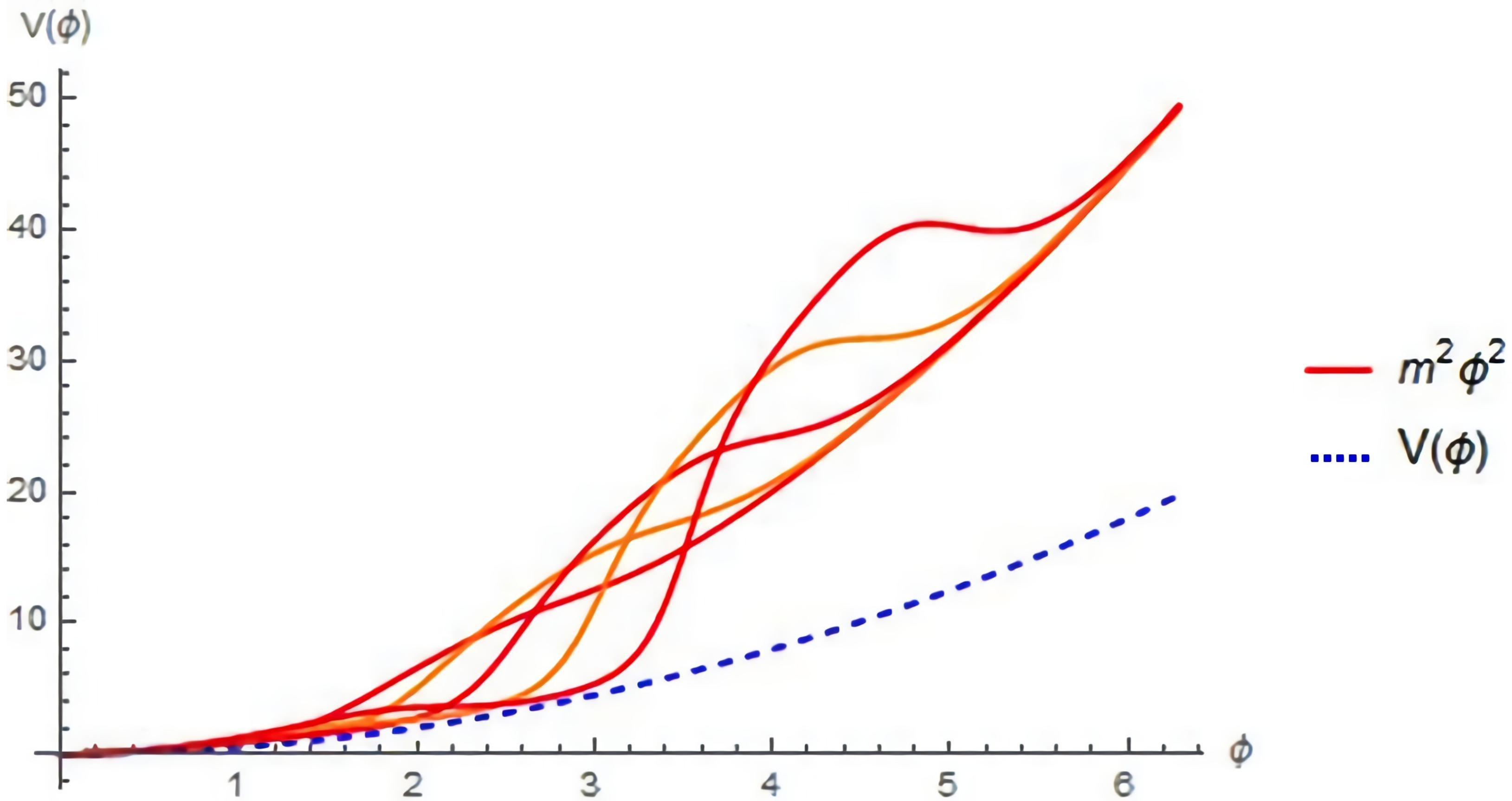
Here, the parameter
is particularly important in describing the phenomenon of pseudo-cycle annihilation. This process can be described in the following way. After the cylindrical end extends enough towards lower energies, it will start folding upon itself leading to a decay geometry leading eventually to some form of cap at low enough energies. As stated before the associated moduli space will decay whenever the approximation leading to
cannot be sustained anymore. For the sake of simplicity, I will consider this process as being governed by a gaussian distribution, modulated by the fact that there is a maximal (albeit large) number of possible pseudo-cycles supported by the geometry. As the pseudo-cycles disappear, the resulting geometry shifts towards one that favours accelerated expansion, after a phase of re-heating which can be seen in
Figure 1.
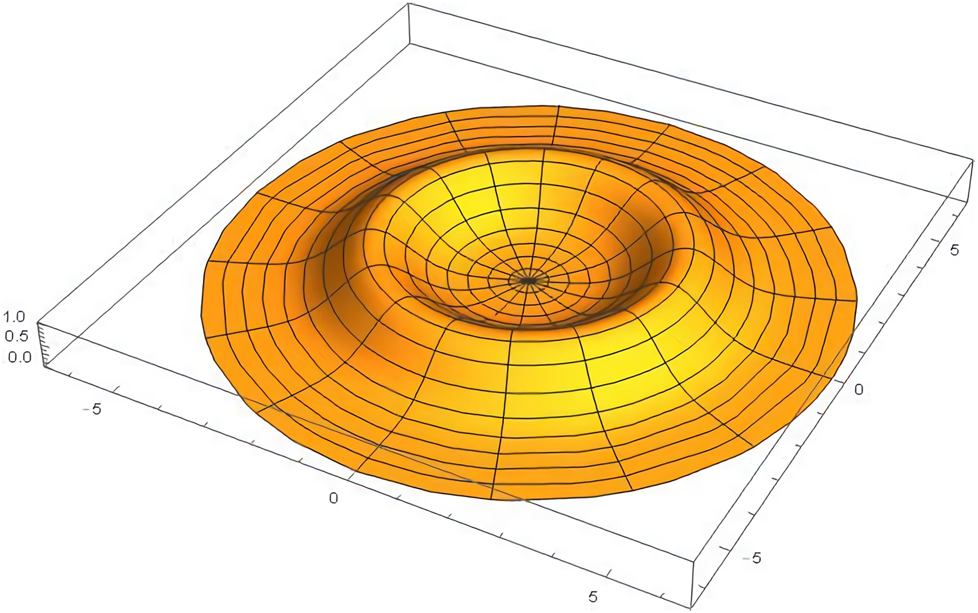
The pseudo-homology identifies a non-trivial component on which non-trivial pseudo-cycles can develop. Its defining parameter is given by the amplitude of the deformation above the flat background, a measure that is decaying as time advances. The construction has been represented in
Figure 2. As the parameter
measures the smoothness of the (pseudo)axion field and the associated potential, it is strongly dependent on the counting of pseudo-cycles in the early universe. This counting can be conducted by means of invariants capable of detecting them, and represents a calculation performed for example in [
47]. Given a moduli space associated to the deformation we introduced, the parameter presented previously in the construction of the extension of the moduli space must be included in the definition of
. Indeed, once the approximation only sees the cylindrical end, the form
restricts to
and the integration follows the method of the standard approach. However, the number of seen axion cycles is substantially increased, being considered as finite, while large, and the resulting cycles as indiscernible given the domain of the approximation. With this in mind, we derive a formula for
playing also the phenomenological role of a continuation function linking the early and the late universe in the form
In this way, we take into account the proliferation of pseudo-cycles in the initial phase, expanding the moduli space accordingly and allowing for new axion-like particles in the early universe, while taking into account their dissipation at a later phase. The maximum number of pseudo-moduli accepted, while large, is finite. Its finite nature will play an important role in the end-stage of the pseudo-cycle proliferation, leading to a re-heating phase controlled by
and by the length of the cylinder section of the distortion. There are several ways in which inflation can be explained by means of an underlying stringy construction. The main approaches involve the lightest scalar fields emerging from string compactifications. These are divided into two main categories: either radial moduli, such as the dilaton and the volume of compactification, which have an unbounded field range in the weak coupling limit. Those, however, contribute to the potential in a very sharp way, unable to produce the type of large-field inflation. Then there are the angular moduli, such as axions, have potentials that are classically protected by shift symmetries, but have within a single period, a very small field range, of the sub-Planckian scale. Those also could not in principle trigger the large-field inflation desired. The solution to this problem was the introduction of a monodromy in the moduli space, a phenomenon that can easily be accounted for by the presence of wrapped branes. This leads to a potential energy that is no longer a periodic function of the axion. Another way of introducing this monodromy was by constructing a theory with axions arising from torsion cycles for example in type IIB compactification. While the introduction of axion monodromy is capable of providing a mechanism for chaotic inflation, the introduction of the torsion in the cycles provides a step-like evolution of the potential as a function of the inflation scalar field arising at a critical scale. The evolution before and after that scale continues to be a quadratic function. Both methods provide no actual mechanism for what we observe, namely an increase of the Hubble parameter at some point in the past, without an alteration of the hot dark matter content that would violate the bounds on structure formation in the universe. The pseudo-axion cycles in the early universe could solve both problems, explaining the discrepancy in the
values measured in the CMB and locally, while not increasing the hot-dark matter density in the later stages. Therefore, the process I went through in the calculation above goes as follows: we start with a type IIB string theory with N D3 branes along the 3+1 dimensional spacetime and a warped 10-dimensional geometry. In the normal situation there is a direct one-to-one relation between the massless modes on a conformal Calabi–Yau and the elements of the cohomology groups of the inner manifold. However, the massless modes are not sensitive to a D-brane wrapping torsional cycles. If we denote the unwrapped internal space by
and the wrapped internal space as
we have two independent torsion classes, the one of torsion 1-cycles and the one of torsion 2-cycles. We may define the generators of the Torsion homology group, and use them to construct the Laplacian eigenforms of
. These will be used to expand the usual IIB gauge forms NS-NS and RR and to calculate the field strengths. With these forms we go back and dimensionally reduce the IIB action on
into a SUGRA type action, impose the tadpole cancellation and obtain the corresponding fluxes by integrating the Bianchi identity and obtain a four dimensional action which, by absorption of various factors into the fields will amount in the action mentioned above. This has mostly been conducted in ref. [
46]. The element that was not discussed in ref. [
46] was the evolution of
which was regarded only as a gluing parameter that would make the jump at the critical value of the field smooth. However, that is the main parameter that is modulated by the presence of pseudocycles in the following way. If the flux coupling varies between the inside and the outside of the wrapped manifold, it leads to a modulation of the critical scale. If the cycle is real, we are free to impose a modulation that may be the best fit to observational data, but we do not have any theoretical restrictions to it. However, in the case of a pseudo-cycle, the inner region has a flux coupling that depends on the field and is limited in spreading to lower energies to the point where the pseudo-cycle actually dissipates. In the torsion monodromy model
depends on the form of the axion potential. If the axions are constructed on pseudo-cycles, its value will disappear after the capping energy of our pseudocycles. This means also that the flux coupling will be different inside the pseudocycle as opposed to outside, in the same way in which it happens for real cycles in the torision triggered monodromy of ref. [
46]. What matters is that those axions will have to decay when the pseudo-cycle geometry dissipates and therefore such a geometry will enhance the specific decay channels. Indeed, if this mechanisms occurs, its effect should be detectable either in the cosmic microwave background as a pseudo-axion decay resonance, or in the spectrum of cosmological gravitational waves.


