Research on Morphological Detection of FR I and FR II Radio Galaxies Based on Improved YOLOv5

Abstract

Recently, astronomy has witnessed great advancements in detectors and telescopes. Imaging data collected by these instruments are organized into very large datasets that form data-oriented astronomy. The imaging data contain many radio galaxies (RGs) that are interesting to astronomers. However, considering that the scale of astronomical databases in the information age is extremely large, a manual search of these galaxies is impractical given the need for manual labor. Therefore, the ability to detect specific types of galaxies largely depends on computer algorithms. Applying machine learning algorithms on large astronomical data sets can more effectively detect galaxies using photometric images. Astronomers are motivated to develop tools that can automatically analyze massive imaging data, including developing an automatic morphological detection of specified radio sources. Galaxy Zoo projects have generated great interest in visually classifying galaxy samples using CNNs. Banfield studied radio morphologies and host galaxies derived from visual inspection in the Radio Galaxy Zoo project. However, there are relatively more studies on galaxy classification, while there are fewer studies on galaxy detection. We develop a galaxy detection model, which realizes the location and classification of Fanaroff–Riley class I (FR I) and Fanaroff–Riley class II (FR II) galaxies. The field of target detection has also developed rapidly since the convolutional neural network was proposed. You Only Look Once: Unified, Real-Time Object Detection (YOLO) is a neural-network-based target detection model proposed by Redmon et al. We made several improvements to the detection effect of dense galaxies based on the original YOLOv5, mainly including the following. (1) We use Varifocal loss, whose function is to weigh positive and negative samples asymmetrically and highlight the main sample of positive samples in the training phase. (2) Our neural network model adds an attention mechanism for the convolution kernel so that the feature extraction network can adjust the size of the receptive field dynamically in deep convolutional neural networks. In this way, our model has good adaptability and effect for identifying galaxies of different sizes on the picture. (3) We use empirical practices suitable for small target detection, such as image segmentation and reducing the stride of the convolutional layers. Apart from the three major contributions and novel points of the model, the thesis also included different data sources, i.e., radio images and optical images, aiming at better classification performance and more accurate positioning. We used optical image data from SDSS, radio image data from FIRST, and label data from FR Is and FR IIs catalogs to create a data set of FR Is and FR IIs. Subsequently, we used the data set to train our improved YOLOv5 model and finally realize the automatic classification and detection of FR Is and FR IIs. Experimental results prove that our improved method achieves better performance. [email protected] of our model reaches 82.3%, and the location (Ra and Dec) of the galaxies can be identified more accurately. Our model has great astronomical significance. For example, it can help astronomers find FR I and FR II galaxies to build a larger-scale galaxy catalog. Our detection method can also be extended to other types of RGs. Thus, astronomers can locate the specific type of galaxies in a considerably shorter time and with minimum human intervention, or it can be combined with other observation data (spectrum and redshift) to explore other properties of the galaxies.

1. Introduction

Extended RGs are traditionally classified according to the Fanaroff–Riley (FR) scheme [1] as FRI and FRII sources. FR class I (FR I) and FR class II (FR II) are two types of RGs with different morphologies. By examining the extended components of the source, the pattern of the surface brightness with different brightness in various regions, we can identify whether it is FR Is or FR IIs [2]. Within the two to half extent of the source of FR Is, small or even no separation can be observed between the points with the highest peak intensities (Figure 1). The regions of jets and core often have the highest level of surface brightness, which is why we say that FR Is have an edge-darkened radio morphology [3]. FR II sources, on the contrary, have separation that can be easily observed between the peak-intensity points (Figure 2). Instead of having a bright region of jets and core, FR IIs have highlighted edges with the highest surface brightness. Therefore, FR IIs have an edge-brightened radio morphology [4]. Studying RGs according to their morphology can help us to understand the galaxies’ formation, evolution, and subcomponents better [2]. Raouf et al. studied the impact of the formation and evolution of radio jets on galaxy evolution [5]. Crotond et al. studied AGN feedback using a high-resolution simulation of the growth of structure in unprecedented detail [6]. Khosroshahi et al. studied the radio emission of the most massive galaxies in a sample of dynamically relaxed and unrelaxed galaxy groups from the Galaxy and Mass Assembly survey [7]. New radio observatories are generating massive imaging data, and the manual inspection is time consuming [8]. The artificial neural network model proposed by Gravet (2015) [9] is a very effective method to classify five types of galaxies, namely a spheroid, a disk, presenting an irregularity, compact or point source, and unclassifiable. Alhassan (2018) [2], using data from FRIST, developed a classifier for Compact, BENT, FRI, and FRII galaxies using a well-trained deep convolutional neural network model (DCNN). However, their approaches are to manually cut out the galaxies of interest from large radio images and then classify RGs by image classification using deep learning models. Cropping single galaxies manually is time consuming and labor intensive; thus, this approach is evidently infeasible for a large number of imaging data. The object detection model only needs to input the original imaging data from radio observatories. Then, it can identify the objects of interest in the image and simultaneously provide the object coordinates (Ra and Dec). Compared with the previous method (Gravet 2015, Alhassan 2018) [2], this approach is equivalent to using model automation instead of manually cropping galaxy images. YOLO [10] is an object detection model that uses deep neural networks. We designed an improved object detector based on the original YOLOv5 [10] and improved the robustness of the model by improving the problem of small target detection. Experiments tested the model through the test set and verified that the performance of the model is significantly better than the original YOLOv5 method. It can achieve higher accuracy and robustness while ensuring the detection speed.

The main objective is to propose a model that automatically performs accurate and robust position and classification prediction for FRI and FRII galaxies. Experimental results show that our object detection model can effectively locate and classify FR I and FR II galaxies. [email protected] reached 82.3%. map[0.05, 0.95] reached 39.3%. The precision and recall were 82.6% and 84.3%, respectively. Our model effectively improves the effect of galaxy detection and classification compared with the original YOLOv5. Our neural network model is developed using the PyTorch deep learning framework.

This paper is organized as follows. In Section 2, the data set is presented. Section 3 presents data preprocessing and augmentation. In Section 4 and Section 5, the object detection algorithm and our network architecture are described. Section 6 presents the model performance evaluation in detail. In Section 7, we present our conclusions and future work.

2. Radio Galaxy Catalog

We use two catalogs to construct our sample of radio sources. Both catalogs provide the source coordinates and classification labels.

For FR Is, the FRICAT catalog by Capetti (2016) [3] is used. The catalog includes data of the Sloan Digital Sky Survey [11], NRAO VLA Sky Survey (NVSS) [12], and Faint Images of the Radio Sky at Twenty-Centimeters (FIRST) [13]. FRICAT includes 219 FR I with redshifts ≤0.15 and an edge-darkened radio morphology with the radius extending larger than 30 kpc from the host. Capetti (2016) [3] investigated the information of radio morphology and the possibility to create the catalog of FR Is selected based on the radio and optical data with the name of FRICAT. We show image examples of FR I galaxies (Figure 1 and Figure 3) in SDSS and FIRST.

For FR IIs, we employed the FRIICAT catalog by Capetti (2017) [4]. FRIICAT includes 122 FR IIs with redshifts ≤0.15 and an edge-brightened radio morphology with at least one of the emission peaks located at the radius r larger than 30 kpc from the center of the host. The image examples of FR II galaxies in SDSS and FIRST are shown in Figure 2 and Figure 4.

3. Image Preprocessing and Data Augmentation

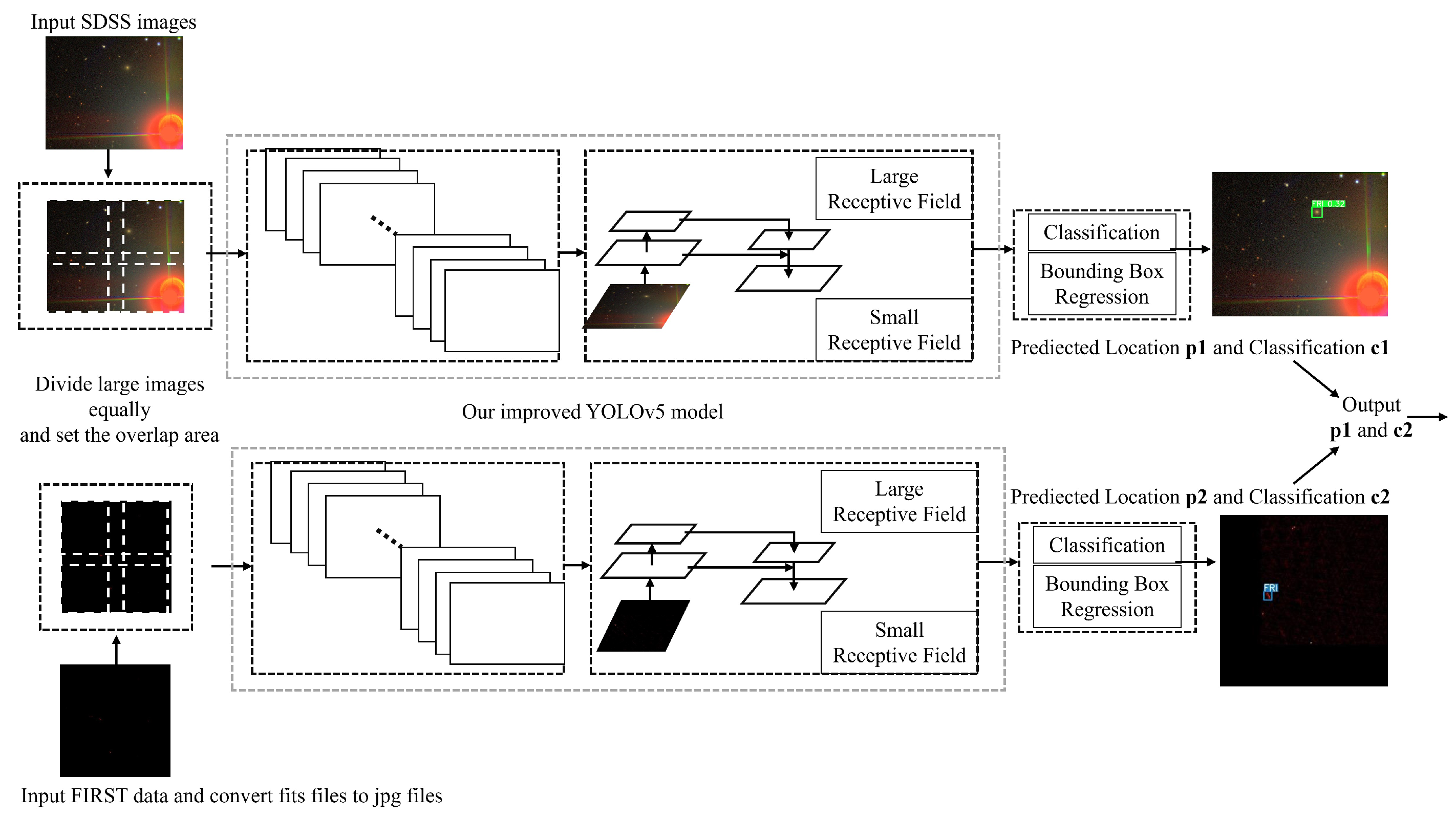
By detecting the source at 1.4 GHz with a resolution of 5 arcseconds and a sensitivity of 1 mJy/bm, nearly one-fourth of the sky was mapped in the FIRST survey [13], of which two areas, the northern area and the southern area, were coincidently covered by the areas detected in another survey, The Sloan Digital Sky Survey [11] (SDSS). SDSS [11] has created the most detailed 3D maps of the universe with deep multicolor images of one-third of the sky. All data are publicly available and can be downloaded1. After downloading the images, we performed image preprocessing and data augmentation. Image data from FIRST were first saved as PNG files [2], then we used the image denoising method of Aniyan and Thorat (2017) [14] for both FIRST data and SDSS data. We deleted, i.e., set all pixel values below 3 $\sigma$ from the median to zero to eliminate background noise, meaning that all values within the range [median-3 $\sigma$, median+3 $\sigma$] were shrunken into zero; therefore, the contribution of the source was highlighted, and the unwanted background noise was removed. Then, we generated artificial images by flipping and rotating to generate sufficient data to train our model due to the small number of labeled images. We adopted a method similar to Alhassan (2018) [2], where each marked image is randomly rotated by an angle and then flipped along the x-axis to generate an artificial image. In addition, in the process of random rotation of the image, we used bilinear interpolation to avoid holes. After the picture was randomly rotated, we discarded the image wherein the target turned out of the canvas because the picture did not contain the target we were interested in. This situation is shown in Figure 5. Flip and rotate do not increase the topological information in the data but change the orientation of the object significantly.

4. Object Detection

The task of object detection is not only to provide the class information of the target to be detected but also to give the position of the target in the image and surround it with the smallest rectangular frame; that is, to achieve the target of classification and positioning. YOLO [10] is an object detection model built with deep neural networks. It was originally used in the COCO data set to detect and classify birds, cats, dogs, horses, sheep, cows, elephants, etc. YOLO has now experienced the development from v1 to v5. Compared with the four previous versions, the YOLOv5 network model has the advantages of small size, fast speed, and high accuracy. Fast R-CNN [15], Faster R-CNN [16], YOLO [10], and SSD [17] have appeared in the field of object detection. Among them, the YOLO algorithm belongs to the end-to-end detection framework. YOLO treats object detection as regression problem solving by using a single end-to-end network so that it can complete the input from the original image to the output of the target position at one time. Its detection performance can achieve real-time processing, which is very suitable for such a large amount of imaging data. Therefore, the YOLO algorithm can be used there to deal with this task and as a baseline of our method. The neural network structure of the YOLOv5 model is shown in Figure 6, wherein each square represents a convolution module formed by stacking several convolution networks. The YOLO algorithm divides the input image into NxN grids, and the grid at the center of the target is responsible for this target. Each candidate box can predict five quantities: x, y, w, h, and l. (x, y) represents the coordinates of the target center point (that is, the center of the galaxy); (w, h) represents the width and height of the box, respectively; l (class) represents the class of the target. To predict these five values at once, the loss function of the YOLOv5 model contains two parts: one part is classification loss, and the other part is regression loss. Among them, the classification loss of the original YOLOv5 is Focal loss, the regression loss of the original YOLOv5 is Intersection over Union (IOU) loss [10].

$$\begin{array}{c}\mathrm{Intersection}\mathrm{over}\mathrm{Union}\left(\mathrm{IOU}\right)=\frac{\mathrm{intersection}}{\mathrm{union}}\hfill \end{array}$$

(1)

As mentioned above, the YOLO algorithm has a smaller number of calculations, faster speed, and higher accuracy. However, certain bottlenecks are still encountered in the detection of small targets, such as RGs. In this regard, Varifocal loss is used instead of the Focal loss in the original YOLOv5 to improve this shortcoming. After training with the data set, our model gained the strong ability to locate and classify galaxies.

5. Our Method

In the radio images, a single galaxy occupies very few pixels in the entire image. The so-called small target has an imaging area of fewer than 80 pixels in a 256 × 256 image based on the definition of the International Society for Optical Engineering. According to this definition, the galaxy can be regarded as a small target in radio images, and this work is a small target detection task. The same situation is faced in optical images. Small targets occupy fewer pixels in the image, the resolution is lower, and the ability to express features is weaker than the conventional size targets. At present, many research directions and related algorithms are available for small target detection tasks, such as presenting attention mechanisms, generating super-resolution feature representation, introducing context information, and processing differences in data sets [19]. Based on these ideas, we made improvements to the original YOLOv5 target detection model that are suitable for small target detection tasks.

First, in our model, the original Focal loss function [20] is replaced with the Varifocal loss function designed by Zhang (2021) [21].

Focal loss, as the name suggests, distinguishes between samples that are difficult to classify and samples that are easy to classify. Focal loss focuses on samples that are difficult to classify, thereby reducing the weight of samples that are easy to classify in the model learning stage. The formula is expressed as:

$$FL(p,y)=\left\{\begin{array}{cc}-\alpha {(1-p)}^{\gamma }log\left(p\right)\hfill & \mathrm{if}y=1\hfill \\ -(1-\alpha )p^{\gamma }log(1-p)\hfill & \mathrm{otherwise}\hfill \end{array}\right.$$

(2)

where p is the classification score, and r is a hyperparameter. The larger the value, the more obvious the distinction between difficult and easy samples. If r is set to 0, then the Focal loss function degenerates into cross-entropy loss.

The new loss function we used is called Varifocal loss, which is expressed as:

$$VFL\left(p,q\right)=\left\{\begin{array}{c}-q\left(qlog\left(p\right)+\left(1-q\right)log\left(1-p\right)\right)\hfill \\ -\alpha p^{\gamma }log\left(1-p\right)\hfill \end{array}\right.\begin{array}{c}q>0\hfill \\ q=0\hfill \end{array}$$

(3)

where p is the predicted Iou-aware classification score (IACS) [21], and q is the IOU score [21] between its ground truth (actual category labels and accurate location in reality) and the generated bounding box. Thus, the training can focus on those high-quality samples. $\alpha$ and $\gamma$ are hyperparameters. $\alpha$ is an adjustable scaling factor to balance the losses between positive and negative examples, and 0 $\le \alpha \le$ 1. Thus, the training can avoid focusing on negative examples. The model can judge and weigh between difficult and easy samples and can ultimately reduce the loss contribution of easy samples because 0 ≤p≤ 1, and $\gamma$ is usually set greater than 1.

Second, we also added the attention mechanism, which provides the model the importance of distinguishing information during training and focuses on the more relevant part of the image features according to training needs. Neural network scientists apply this mechanism, which is similar to the human visual selection mechanism, to neural networks. The attention mechanism will enable it to make targeted selections when extracting the features of the input samples and assign higher weights to the features that are beneficial to the training of the network model. Features that do not affect the performance of the network model or are even unfavorable for network training are assigned lower weights. The SKnet module [22] used in this paper is the attention mechanism for the convolution kernel. In addition, the attention mechanism includes the attention mechanisms for the space and the channel. SKnet [22] is inspired by the instance wherein the size of the human receptive field of visual cortex neurons is adjusted according to the stimulus when looking at objects of different sizes. Therefore, SKnet realizes that if the galaxy of interest in the picture is relatively large (occupying more pixels), then the neural network convolution layer will be more inclined to select a larger convolution kernel (for larger convolution kernel convolution). The feature map obtained by the product is assigned a higher weight. If the galaxy is relatively small, then the neural network convolution layer will be more inclined to opt for a smaller convolution kernel (feature obtained by convolution of the smaller convolution kernel map assigns a higher weight). This mechanism is called the attention mechanism for the convolution kernel because it adaptively adjusts the size of the convolution kernel according to the input. The SKConv module in our model is added with SKnet [22]; thus, each neuron automatically adjusts the receptive field [23] according to the input image and integrates shallow and deep features, thereby considerably improving the accuracy of our galaxy detection model. The structure diagram of SKnet is shown in Figure 7.

The SKConv module enables each neuron to adjust the receptive field automatically according to the input information. The neural network structure of our model is shown in Figure 8.

Third, the shallow feature map in the neural network contains rich, detailed information, which is more conducive to detecting small targets. Therefore, our model adopts the method of Ju et al. [24], decreases the number of pooling layers to avoid downsampling, and uses a shallower convolutional network. In addition, our model refers to the method of van Etten et al. [25]. We reduced the stride of the convolutional layer to allow our model to become more conducive to small target detection. Furthermore, we used the method in the YOLT algorithm [25] to divide large-resolution images equally and set the overlap area (to prevent some targets from being segmented and truncated); then, we input them into the neural network. The process from input to output is shown in Figure 9.

6. Experiment and Results

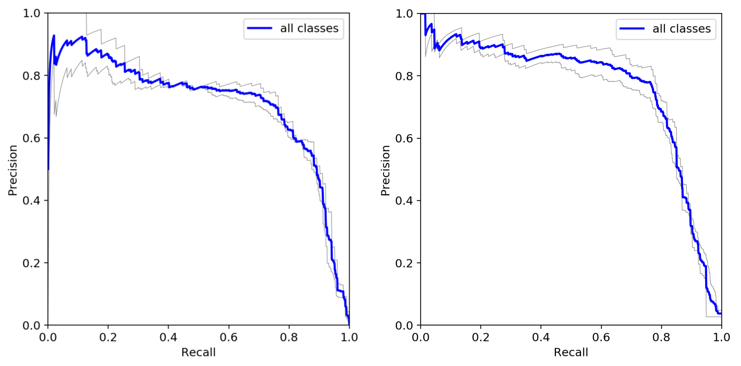
6.1. Metrics and Quantitative Experimental Results

To assess how accurately the model can predict the classes and locations of different morphology galaxies, the precision (P), recall (R), and [email protected] were calculated using the test data set based on the number of true-positive (TP), false-positive (FP), and false-negative (FN) detection, as given below:

$$\begin{array}{c}\mathrm{Recall}=\frac{TP}{TP+FN}\hfill \\ \mathrm{Precision}=\frac{TP}{TP+FP}\hfill \end{array}$$

(4)

where

(i)

TP means that when we predict the source as FRII and it is FRII in fact. It also satisfies that the IOUs of the prediction box and the ground truth box are greater than 0.5.

(ii)

FP means that when we predict the source as FRII but it is not FRII in fact. It also satisfies that the IOUs of the prediction box and the ground truth box are less than 0.5.

(iii)

FN means that when we predict the source as not FRII but it is FRII in fact. It also satisfies that the IOUs of the prediction box and the ground truth box are greater than 0.5.

P in AP and in [email protected] stands for Precision. AP is the abbreviation of average precision, which refers to the accuracy rate of a single class label. [email protected] is the abbreviation of mean average precision, which corresponds to the mean of average precision of all classes. The [email protected] in the target detection is calculated as follows. For the samples in the test set, if the IOU of the prediction box and the ground truth box is greater than 0.5, then the two boxes match. On this basis, the samples whose prediction scores outputted in the upper right corner of the box are greater than the threshold are predicted as positive samples (marked with boxes in the figure). Precision and recall at this time can be calculated according to Formula (4). Different positive samples can be obtained by adjusting the threshold so that different (P, R) values can be calculated. The precision–recall curve (P–R curve) is utilized to trace these (P,R) points in the coordinate system and connect them into a line. The area under a P–R curve that corresponds to each class is defined as the AP of this class, and the average value of AP of all classes is taken to obtain [email protected]. map[0.5:0.95], which is the mean when the threshold of IOU is set to 0.5, 0.55, 0.6, 0.65, 0.7, 0.75, 0.8, 0.85, 0.9, and 0.95. On a target detection task, the most important and most scientific indicator is mAP [26] (that is, the area under the all-classes P–R curve). Thus, if the all-classes P–R curve of a model wraps the all-classes P–R curve of the original model completely, then the model is better than the original one. In the figure, our model is better than the original model. map[0.5:0.95] is an evaluation index that necessitates higher requirements for the position of the prediction frame. map[0.5:0.95] of our model is larger than the original model, indicating that our model predicts the position of the galaxy more accurately. Figure 10 shows our P–R curve on the original YOLOv5 and our improved model.

Table 1. mAP, accuracy, and recall of YOLOv5 and our model.

Method	[email protected]	map[0.5:0.95]	Precision	Recall
Yolov5	74.8	35.1	78.1	80.5
Our Model	82.3	39.3	82.6	84.3

shows mAP, precision, and recall of two models.

Table 2. Hyperparameters used to train our model.

Hyperparameters	Values
Batch Size	16
Dropout Rate	0.5
Epochs	400

shows the hyperparameters used to train our model. The effects of our galaxy detection model are shown in Figure 11 and Figure 12.

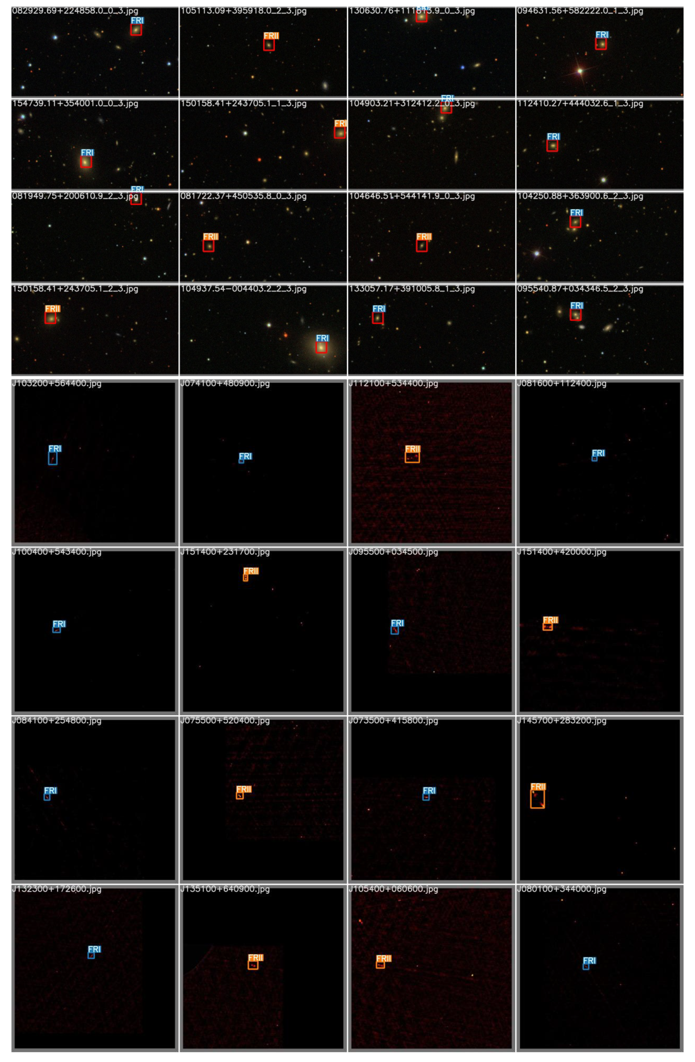
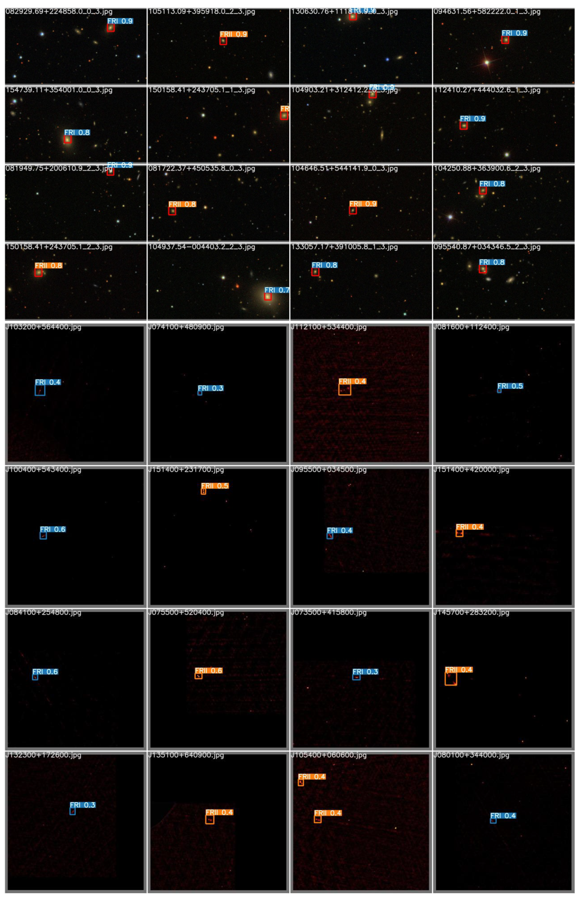
6.2. Results and Effects

In order to evaluate the effectiveness of our improved object detection model in comparison with the ground truth, we selected random FR I and FR II galaxy image samples detected by our improved object detection model, as shown in

Table 3. Comparison between our model predictions and the ground truth of some samples.

Course		Ground Truth			Model Prediction
	Ra (deg)	Dec (deg)	True Class	Predicted Ra (deg)	Predicted Dec (deg)	Predicted Class
	119.06145833	50.36669444	FR II	119.061458	50.366694	FR II
	145.36895833	39.69252778	FR II	145.368958	39.692528	FR II
	162.80454167	39.98833333	FR II	162.804542	39.988333	FR II
	181.92404167	33.80716666	FR II	181.924041	33.807166	FR II
	224.48295833	28.49813889	FR II	224.482958	28.498139	FR II
	115.37591666	48.07438889	FR I	115.375917	48.074389	FR I
	124.04991667	43.04966667	FR I	124.049916	43.049667	FR I
	124.72800000	4.05211111	FR I	124.728000	4.052111	FR I
	242.10225000	37.65530556	FR I	242.102250	37.655306	FR I
	247.02729167	8.69638889	FR I	247.027291	8.696389	FR I

. These samples show that our model is very accurate in positioning and has achieved good results in classification. It can be applied to the pipeline of the data processing of survey telescopes.

7. Conclusions

Automatic detection of specified objects is greatly required in upcoming massive RG images. We propose an improved galaxy detection model based on YOLOv5 to automatically locate and classify the FR I and FR II RGs. This is a great convenience for discovering and measuring their positions, exploring their laws of motion, and studying their physical properties, chemical composition, internal structure, and their evolutionary laws. Innovations and improvements in three aspects result in considerable performance improvement to the original YOLOv5. In addition, our model has achieved good experimental results, proving the accuracy and robustness of our method. In the future, we will improve the model’s ability to obtain detailed information from galaxy images and further improve the accuracy of classification and positioning. We will also expand the data set so that the model can classify and locate more types of galaxies (such as BENT and Compact).

References

1. Fanaroff, B.L.; Riley, J.M. The Morphology of Extragalactic Radio Sources of High and Low Luminosity. Mon. Not. R. Astron. Soc. 1974, 167, 31P–36P. [Google Scholar] [CrossRef] [Green Version]
2. Alhassan, W.; Taylor, A.R.; Vaccari, M. The FIRST Classifier: Compact and Extended Radio Galaxy Classification using Deep Convolutional Neural Networks. MNRAS 2018, 480, 2085–2093. [Google Scholar] [CrossRef] [Green Version]
3. Baldi, R.D.; Capetti, A.; Massaro, F. FRICAT: A FIRST catalog of FR I radio galaxies. Astron. Astrophys. 2017, 598, A49. [Google Scholar]
4. Capetti, A.; Massaro, F.; Baldi, R.D. FRIICAT: A FIRST catalog of FR II radio galaxies. Astron. Astrophys. 2017, 601, 1–10. [Google Scholar] [CrossRef] [Green Version]
5. Raouf, M.; Shabala, S.S.; Croton, D.J.; Khosroshahi, H.G.; Bernyk, M. The many lives of active galactic nuclei–II: The formation and evolution of radio jets and their impact on galaxy evolution. Mon. Not. R. Astron. Soc. 2017, 471, 658–670. [Google Scholar] [CrossRef] [Green Version]
6. Croton, D.J.; Volker, S.; White, S.; De, L.G.; Frenk, C.S.; Gao, L.; Jenkins, A.; Kauffmann, G.; Navarro, J.F.; Yoshida, N. The many lives of active galactic nuclei: Cooling flows, black holes and the luminosities and colours of galaxies. Mon. Not. R. Astron. Soc. 2010, 365, 11–28. [Google Scholar] [CrossRef] [Green Version]
7. Khosroshahi, H.G.; Raouf, M.; Miraghaei, H.; Brough, S.; Croton, D.J.; Driver, S.; Graham, A.; Baldry, I.; Brown, M.; Prescott, M. Galaxy And Mass Assembly (GAMA): ‘No Smoking’ zone for giant elliptical galaxies? Astrophys. J. 2017, 842, 81. [Google Scholar] [CrossRef] [Green Version]
8. Hocking, A.; Geach, J.E.; Davey, N.; Yi, S. Teaching a machine to see: Unsupervised image segmentation and categorisation using growing neural gas and hierarchical clustering. Physics 2015, 23, 619–620. [Google Scholar]
9. Gravet, R.; Cabrera-Vives, G.; Pérez-González, P.G.; Kartaltepe, J.S.; Barro, G.; Bernardi, M.; Mei, S.; Shankar, F.; Dimauro, P.; Bell, E.F.; et al. A catalog of visual-like morphologies in the 5 CANDELS fields using deep-learning. Astrophys. J. Suppl. Ser. 2015, 221, 8. [Google Scholar]
10. Redmon, J.; Divvala, S.; Girshick, R.; Farhadi, A. You Only Look Once: Unified, Real-Time Object Detection; IEEE: New York, NY, USA, 2016. [Google Scholar]
11. York, D.G.; Adelman, J.; Anderson, J.E., Jr.; Anderson, S.F.; Annis, J.; Bahcall, N.A.; Bakken, J.A.; Barkhouser, R.; Bastian, S.; Berman, E.; et al. The Sloan Digital Sky Survey: Technical Summary. Astron. J. 2000, 120, 1579. [Google Scholar] [CrossRef]
12. Library, W.E. The Astronomical Journal; American Institute of Physics: College Park, MD, USA, 1997. [Google Scholar]
13. Becker, R.H.; White, R.L.; Helfand, D.J. The FIRST survey: Faint Images of the Radio Sky at Twenty centimeters. Astrophys. J. 1995, 450, 559. [Google Scholar] [CrossRef]
14. Aniyan, A.K.; Thorat, K. Classifying Radio Galaxies with the Convolutional Neural Network. Astrophys. J. Suppl. 2017, 230, 20. [Google Scholar] [CrossRef]
15. Girshick, R. Fast R-CNN. In Proceedings of the IEEE International Conference on Computer Vision (ICCV), Santiago, Chile, 7–13 December 2015; pp. 1440–1448. [Google Scholar]
16. Ren, S.; He, K.; Girshick, R.; Sun, J. Faster R-CNN: Towards Real-Time Object Detection with Region Proposal Networks. IEEE Trans. Pattern Anal. Mach. Intell. 2017, 39, 1137–1149. [Google Scholar] [CrossRef] [PubMed] [Green Version]
17. Liu, W.; Anguelov, D.; Erhan, D.; Szegedy, C.; Reed, S.; Fu, C.Y.; Berg, A.C. SSD: Single Shot MultiBox Detector; Springer: Cham, Switzerland, 2016. [Google Scholar]
18. Shu, L.; Zhang, Z.; Lei, B. Research on Dense-Yolov5 Algorithm for Infrared Target Detection. Opt. Optoelectron. Technol. 2021, 19, 69–75. [Google Scholar]
19. Zhou, X.C.; Gong, J.H.; Yun-Qian, L.I.; Chen, X.J. Research Progress of Malicious Code Detection Technology Based on Deep Learning. Mod. Comput. 2019. [Google Scholar]
20. Lin, T.Y.; Goyal, P.; Girshick, R.; He, K.; Dollár, P. Focal Loss for Dense Object Detection. In IEEE Transactions on Pattern Analysis & Machine Intelligence; IEEE: New York, NY, USA, 2017; pp. 2999–3007. [Google Scholar]
21. Zhang, H.; Wang, Y.; Dayoub, F.; Sünderhauf, N. VarifocalNet: An IoU-aware Dense Object Detector. In Proceedings of the IEEE/CVF Conference on Computer Vision and Pattern Recognition, Colorado Springs, CO, USA, 20–25 June 2020. [Google Scholar]
22. Li, X.; Wang, W.; Hu, X.; Yang, J. Selective Kernel Networks. In Proceedings of the 2019 IEEE/CVF Conference on Computer Vision and Pattern Recognition (CVPR), Long Beach, CA, USA, 15–20 June 2019. [Google Scholar]
23. Liu, X.; Wang, Z.; He, Y.; Liu, Q. Research on Small Target Detection Based on Deep Learning. Tactical Missile Technol. 2019. [Google Scholar]
24. Ju, M.; Luo, H.; Wang, Z. Improved YOLOv3 Algorithm and Application in Small Target Detection. Acta Opt. 2019, 39, 245–252. [Google Scholar]
25. Etten, A.V. You Only Look Twice: Rapid Multi-Scale Object Detection in Satellite Imagery. arXiv 2018, arXiv:1805.09512. [Google Scholar]
26. Everingham, M.; Eslami, S.M.; Gool, L.; Williams, C.K.; Winn, J.; Zisserman, A. The Pascal Visual Object Classes Challenge: A Retrospective. Int. J. Comput. Vis. 2015, 111, 98–136. [Google Scholar] [CrossRef]
1.
https://www.sdss.org/ (accessed on 10 October 2020).
Figure 1. J0039-1032 J1053+4929 J0140+0018 J0152-0010 J1053+4929. Examples of radio morphologies of FR Is. These images are drawn from 0.45 mJy/beam and increase in geometric progression at the same ratio of 2 .
Universe 07 00211 g001
Figure 2. J1102+2429 J1131+6047 J1620+4309 J1054+0606 J1102+2907. Examples of radio morphologies of FR IIs. These images are drawn from 0.45 mJy/beam and increase in geometric progression at the same ratio of 2 .
Universe 07 00211 g002
Figure 3. Image example of an FR I in SDSS and in FIRST.
Universe 07 00211 g003
Figure 4. Image example of an FR II galaxy in SDSS and in FIRST.
Universe 07 00211 g004
Figure 5. The image before random rotation, and the image after random rotation. In this case, the galaxy of interest is rotated out, so this picture needs to be discarded. Images before and after random rotation. In this case, the galaxy of interest is rotated out, so this picture needs to be discarded. To provide a clear description, we deliberately marked the galaxies of interest in green in this picture.
Universe 07 00211 g005
Figure 6. The neural network structure of the original YOLOv5 model [18]. Each rectangle or trapezoid represents a module that is encapsulated by several connected single-layer neural networks. Among them, the CSP neural network module performs three convolutions on the feature map and then uses four different scales of max pooling for processing. The kernel sizes are 13 × 13 ,   9 × 9 ,   5 × 5 , and 1 × 1 pixels. They are used to catch the most significant contextual features. The convolutional neural network module is an encapsulated convolution module that includes convolution, activation, and pool operation, whose main function is to extract image features.
Universe 07 00211 g006
Figure 7. Structural diagram of SKnet. The stacked rectangles represent the feature map, and the feature map refers to the output of each layer in the neural network. The unique function of SKnet, the dynamic adjustment of the receptive field, is achieved through three steps: split, fuse, and select. Split refers to the convolution operation with small- and big-sized kernels performed on the input feature map. Fuse refers to the global average pooling operation (global average pooling neural network layer) and fully connected operation (fully connected neural network layer) on the feature map to obtain global information and then embed the global information into a vector. In the select stage, the a and b vectors are used as the weights of the upper and lower branches, and multiplication is performed to achieve the weighting of the upper and lower feature maps. Then, the feature maps of the last two branches are added together and outputted to the next network layer.
Universe 07 00211 g007
Figure 8. Neural network structure of SKConv section. The comparison of Figure 6 and Figure 8 shows that we added SKConv to our model. SKConv includes the attention mechanism SKnet. The Conv, SPP, and Concat modules are originally available in the original YOLOv5 and represent the convolutional modules stacked up by convolutional neural networks for feature extraction.
Universe 07 00211 g008
Figure 9. This illustration represents the whole process; that is, from input to image preprocessing to target detection model to output. We train our improved YOLOv5 models on the SDSS data and FIRST data separately. In this way, we obtain two models, namely the galaxy detection model based on the improved YOLOv5 using radio image data and the galaxy detection model based on the improved YOLOv5 using optical image data. This method as shown in the figure allows us to obtain more accurate positioning and more precise classification when detecting galaxies.
Universe 07 00211 g009
Figure 10. P–R curve of the original YOLOv5 and P–R curve of our model. In object detection that needs to recognize multiple classes, each class draws a curve, whose abscissa and ordinate are recall and precision, respectively. The blue curve represents the P–R curve of all types, and the area under this curve is the most commonly used index for the evaluation of target detection, mAP.
Universe 07 00211 g010
Figure 11. Ground truth of samples in SDSS and FIRST images.
Universe 07 00211 g011
Figure 12. Predicted samples in SDSS and FIRST images. The prediction box is drawn on the basis of the values of x, y, w, and h predicted by our neural network model. The string and decimal in the upper right corner of each prediction box is the predicted class and confidence score. The closer the score is to 1, the closer the prediction is to the ground truth.
Universe 07 00211 g012