
Multi-Field versus Single-Field in the Supergravity Models of Inflation and Primordial Black Holes †


Abstract
1. Introduction
2. Motivation and Setup
2.1. Why Inflation?
2.2. Why Starobinsky’s Model for Single-Field Inflation?
- the model is geometrical, being based on gravitational interactions;
- its inflaton (called scalaron) is a physical excitation of higher-derivative gravity, so it is not a new fundamental scalar (minimal tool);
- the model has no free parameters after fixing its only parameter M by observations;
- the Starobinsky inflation obeys the Einstein criterium: “simple but not too simple”;
- the UV-cutoff of quantized gravity is given by , as is clear from expanding the non-renormalizable scalar potential (12) in powers of ; this feature ensures reasonable protection of the Starobinsky inflation on the scale GeV against quantum gravity corrections expected near the Planck scale ; and
- rewriting the scalar potential (12) to the form of a mass term by the field redefinitionleads to a non-canonical kinetic term of the field , with the pre-factor having a singularity at and specified by the critical exponentdefining the universality class of the Starobinsky inflation.
- its fundamental origin in quantum gravity or in string theory is unknown;
- it cannot be applied for large negative values of the scalar curvature, when ; and
2.3. Why Primordial Black Holes?
2.4. Why Supergravity?
- SUSY unifies bosons and fermions;
- supergravity includes GR;
- SUSY Grand Unified Theories (super-GUT) lead to the perfect unification of electro-weak and strong interactions;
- the spectrum of matter-coupled supergravities with spontaneously broken SUSY has the natural DM candidate given by the Lightest SUSY Particle (LSP) provided that R-parity is conserved;
- low-energy SUSY helps to stabilize the fundamental scales (the hierarchy problem), such as the electro-weak scale and the GUT scale;
- SUSY leads to cancellation of quadratic UV-divergences in quantum field theory;
- supergravity is the only way to consistently describe spin-3/2 particles with gravity; and
- supergravity arises as the low-energy effective action of superstrings.
3. Single-Field Models
3.1. Power Spectrum and Generalized Alpha Attractors
3.2. Single-Field Models of Inflation and PBH in Supergravity
4. Two-Field Models in Modified Supergravity
4.1. Modified (Starobinsky-Type) Supergravity
4.2. The Effective Two-Field Models
4.3. The Models
4.4. The Models
4.5. Comparison of the and Models with the Observational Constraints on PBH and DM
5. Gravitational Waves Induced by PBH Formation
6. Conclusions and Discussion
Funding
Institutional Review Board Statement
Informed Consent Statement
Acknowledgments
Conflicts of Interest
References
- Ketov, S.V.; Starobinsky, A.A. Embedding (R+R2)-Inflation into Supergravity. Phys. Rev. D 2011, 83, 063512. [Google Scholar] [CrossRef]
- Starobinsky, A.A. A new type of isotropic cosmological models without singularity. Phys. Lett. B 1980, 91, 99–102. [Google Scholar] [CrossRef]
- Novikov, I.; Zeldovic, Y. Cosmology. Ann. Rev. Astron. Astrophys. 1967, 5, 627–649. [Google Scholar] [CrossRef]
- Hawking, S. Gravitationally collapsed objects of very low mass. Mon. Not. Roy. Astron. Soc. 1971, 152, 75. [Google Scholar] [CrossRef]
- Carr, B.J. The Primordial black hole mass spectrum. Astrophys. J. 1975, 201, 1–19. [Google Scholar] [CrossRef]
- Barrow, J.D.; Copeland, E.J.; Liddle, A.R. The Cosmology of black hole relics. Phys. Rev. D 1992, 46, 645–657. [Google Scholar] [CrossRef] [PubMed]
- Sasaki, M.; Suyama, T.; Tanaka, T.; Yokoyama, S. Primordial black holes—Perspectives in gravitational wave astronomy. Class. Quant. Grav. 2018, 35, 063001. [Google Scholar] [CrossRef]
- Ketov, S.V.; Khlopov, M.Y. Cosmological Probes of Supersymmetric Field Theory Models at Superhigh Energy Scales. Symmetry 2019, 11, 511. [Google Scholar] [CrossRef]
- Carr, B.; Kohri, K.; Sendouda, Y.; Yokoyama, J. Constraints on Primordial Black Holes. arXiv 2020, arXiv:2002.12778. [Google Scholar]
- Guth, A.H. The Inflationary Universe: A Possible Solution to the Horizon and Flatness Problems. Phys. Rev. D 1981, 23, 347–356. [Google Scholar] [CrossRef]
- Linde, A.D. A New Inflationary Universe Scenario: A Possible Solution of the Horizon, Flatness, Homogeneity, Isotropy and Primordial Monopole Problems. Phys. Lett. B 1982, 108, 389–393. [Google Scholar] [CrossRef]
- Akrami, Y.; Arroja, F.; Ashdown, M.; Aumont, J.; Baccigalupi, C.; Ballardini, M.; Banday, A.J.; Barreiro, R.B.; Bartolo, N.; Basak, S.; et al. Planck 2018 results. X. Constraints on inflation. arXiv 2020, arXiv:1807.06211. [Google Scholar]
- Ketov, S.V. Quantum Nonlinear Sigma Models: From Quantum Field Theory to Supersymmetry, Conformal Field Theory, Black Holes and Strings; Springer: Berlin, Germany, 2000. [Google Scholar]
- Aldabergenov, Y.; Ishikawa, R.; Ketov, S.V.; Kruglov, S.I. Beyond Starobinsky inflation. Phys. Rev. D 2018, 98, 083511. [Google Scholar] [CrossRef]
- Ketov, S.V. On the equivalence of Starobinsky and Higgs inflationary models in gravity and supergravity. J. Phys. A 2020, 53, 084001. [Google Scholar] [CrossRef]
- Ketov, S.V.; Watanabe, N. On the Higgs-like Quintessence for Dark Energy. Mod. Phys. Lett. A 2014, 29, 1450117. [Google Scholar] [CrossRef]
- Ellis, J.; Garcia, M.A.G.; Nanopoulos, D.V.; Olive, K.A. Calculations of Inflaton Decays and Reheating: With Applications to No-Scale Inflation Models. JCAP 2015, 07, 050. [Google Scholar] [CrossRef]
- Mukhanov, V.F.; Chibisov, G.V. Quantum Fluctuations and a Nonsingular Universe. JETP Lett. 1981, 33, 532–535. [Google Scholar]
- Kaneda, S.; Ketov, S.V.; Watanabe, N. Fourth-order gravity as the inflationary model revisited. Mod. Phys. Lett. A 2010, 25, 2753–2762. [Google Scholar] [CrossRef]
- Ketov, S.V.; Starobinsky, A.A. Inflation and non-minimal scalar-curvature coupling in gravity and supergravity. JCAP 2012, 08, 022. [Google Scholar] [CrossRef]
- Dolgov, A.; Silk, J. Baryon isocurvature fluctuations at small scales and baryonic dark matter. Phys. Rev. D 1993, 47, 4244–4255. [Google Scholar] [CrossRef]
- Ivanov, P.; Naselsky, P.; Novikov, I. Inflation and primordial black holes as dark matter. Phys. Rev. D 1994, 50, 7173–7178. [Google Scholar] [CrossRef]
- Dine, M.; Fischler, W. The Not So Harmless Axion. Phys. Lett. B 1983, 120, 137–141. [Google Scholar] [CrossRef]
- Addazi, A.; Ketov, S.V.; Khlopov, M.Y. Gravitino and Polonyi production in supergravity. Eur. Phys. J. C 2018, 78, 642. [Google Scholar] [CrossRef]
- Bañados, E.; Venemans, B.P.; Mazzucchelli, C.; Farina, E.P.; Walter, F.; Wang, F.; Decarli, R.; Stern, D.; Fan, X.; Davies, F.B.; et al. An 800-million-solar-mass black hole in a significantly neutral Universe at redshift 7.5. Nature 2018, 553, 7689. [Google Scholar] [CrossRef]
- Duechting, N. Supermassive black holes from primordial black hole seeds. Phys. Rev. D 2004, 70, 064015. [Google Scholar] [CrossRef]
- Khlopov, M.; Malomed, B.; Zeldovich, I. Gravitational instability of scalar fields and formation of primordial black holes. Mon. Not. R. Astron. Soc. 1985, 215, 575–589. [Google Scholar] [CrossRef]
- Konoplich, R.; Rubin, S.; Sakharov, A.; Khlopov, M. Formation of black holes in first-order phase transitions as a cosmological test of symmetry-breaking mechanisms. Phys. Atom. Nucl. 1999, 62, 1593–1600. [Google Scholar]
- Khlopov, M.; Konoplich, R.; Rubin, S.; Sakharov, A. First-order phase transitions as a source of black holes in the early universe. Grav. Cosmol. 2000, 6, 153–156. [Google Scholar]
- Addazi, A.; Marcianò, A.; Pasechnik, R. Probing Trans-electroweak First Order Phase Transitions from Gravitational Waves. Physics 2019, 1, 92–102. [Google Scholar] [CrossRef]
- Vilenkin, A.; Levin, Y.; Gruzinov, A. Cosmic strings and primordial black holes. JCAP 2018, 11, 008. [Google Scholar] [CrossRef]
- Belotsky, K.M.; Dokuchaev, V.I.; Eroshenko, Y.N.; Esipova, E.A.; Khlopov, M.Y.; Khromykh, L.A.; Kirillov, A.A.; Nikulin, V.V.; Rubin, S.G.; Svadkovsky, I.V. Clusters of primordial black holes. Eur. Phys. J. C 2019, 79, 246. [Google Scholar] [CrossRef]
- Liu, J.; Guo, Z.-K.; Cai, R.-G. Primordial Black Holes from Cosmic Domain Walls. Phys. Rev. D 2020, 101, 023513. [Google Scholar] [CrossRef]
- Carr, B.J. Primordial black holes as a probe of cosmology and high energy physics. Lect. Notes Phys. 2003, 631, 301–321. [Google Scholar]
- Pi, S.; Zhang, Y.-l.; Huang, Q.-G.; Sasaki, M. Scalaron from R2-gravity as a heavy field. JCAP 2018, 05, 042. [Google Scholar] [CrossRef]
- Germani, C.; Musco, I. Abundance of Primordial Black Holes Depends on the Shape of the Inflationary Power Spectrum. Phys. Rev. Lett. 2019, 122, 141302. [Google Scholar] [CrossRef]
- Fumagalli, J.; Renaux-Petel, S.; Ronayne, J.W.; Witkowski, L.T. Turning in the landscape: A new mechanism for generating Primordial Black Holes. arXiv 2020, arXiv:2004.08369. [Google Scholar]
- Palma, G.A.; Sypsas, S.; Zenteno, C. Seeding primordial black holes in multifield inflation. Phys. Rev. Lett. 2020, 125, 121301. [Google Scholar] [CrossRef]
- Cai, R.-G.; Guo, Z.-K.; Liu, J.; Liu, L.; Yang, X.-Y. Primordial black holes and gravitational waves from parametric amplification of curvature perturbations. JCAP 2020, 06, 013. [Google Scholar] [CrossRef]
- Cai, R.-G.; Pi, S.; Sasaki, M. Gravitational Waves Induced by non-Gaussian Scalar Perturbations. Phys. Rev. Lett. 2019, 122, 201101. [Google Scholar] [CrossRef]
- Deng, C.-M.; Cai, Y.; Wu, X.-F.; Liang, E.-W. Fast Radio Bursts From Primordial Black Hole Binaries Coalescence. Phys. Rev. D 2018, 98, 123016. [Google Scholar] [CrossRef]
- Abbott, B.P.; Abbott, R.; Abbott, T.D.; Abraham, S.; Acernese, F.; Ackley, K.; Adams, C.; Adhikari, R.X.; Adya, V.B.; Affeldt, C.; et al. GWTC-1: A Gravitational-Wave Transient Catalog of Compact Binary Mergers Observed by LIGO and Virgo during the First and Second Observing Runs. Phys. Rev. X 2019, 9, 031040. [Google Scholar] [CrossRef]
- Passaglia, S.; Hu, W.; Motohashi, H. Primordial black holes and local non-Gaussianity in canonical inflation. Phys. Rev. D 2019, 99, 043536. [Google Scholar] [CrossRef]
- Garcia-Bellido, J.; Morales, E.R. Primordial black holes from single field models of inflation. Phys. Dark Univ. 2017, 18, 47–54. [Google Scholar] [CrossRef]
- Motohashi, H.; Hu, W. Primordial Black Holes and Slow-Roll Violation. Phys. Rev. D 2017, 96, 063503. [Google Scholar] [CrossRef]
- Braglia, M.; Hazra, D.K.; Finelli, F.; Smoot, G.F.; Starobinsky, A.A. Generating PBHs and small-scale GWs in two-field models of inflation. arXiv 2020, arXiv:2005.02895. [Google Scholar] [CrossRef]
- Garcia-Bellido, J.; Linde, A.D.; Wands, D. Density perturbations and black hole formation in hybrid inflation. Phys. Rev. D 1996, 54, 6040–6058. [Google Scholar] [CrossRef]
- Kawasaki, M.; Tada, Y. Can massive primordial black holes be produced in mild waterfall hybrid inflation? JCAP 2016, 08, 041. [Google Scholar] [CrossRef]
- Ketov, S.V.; Terada, T. Old-minimal supergravity models of inflation. JHEP 2013, 12, 040. [Google Scholar] [CrossRef]
- Addazi, A.; Ketov, S.V. Energy conditions in Starobinsky supergravity. JCAP 2017, 03, 061. [Google Scholar] [CrossRef]
- Starobinsky, A.A. Spectrum of relict gravitational radiation and the early state of the universe. JETP Lett. 1979, 30, 682–685. [Google Scholar]
- Kallosh, R.; Linde, A.; Roest, D. Superconformal Inflationary α-Attractors. JHEP 2013, 11, 198. [Google Scholar] [CrossRef]
- Dalianis, I.; Kehagias, A.; Tringas, G. Primordial black holes from α-attractors. JCAP 2019, 01, 037. [Google Scholar] [CrossRef]
- Freedman, D.Z.; Proeyen, A.V. Supergravity; Cambridge University Press: Cambridge, UK, 2012. [Google Scholar]
- Wess, J.; Bagger, J. Supersymmetry and Supergravity; Princeton University Press: Princeton, NJ, USA, 1992. [Google Scholar]
- Yamaguchi, M. Supergravity based inflation models: A review. Class. Quant. Grav. 2011, 28, 103001. [Google Scholar] [CrossRef]
- Ketov, S.V. Supergravity and Early Universe: The Meeting Point of Cosmology and High-Energy Physics. Int. J. Mod. Phys. A 2013, 28, 1330021. [Google Scholar] [CrossRef]
- Ketov, S.V.; Terada, T. Inflation in supergravity with a single chiral superfield. Phys. Lett. B 2014, 736, 272–277. [Google Scholar] [CrossRef]
- Ketov, S.V.; Terada, T. Generic Scalar Potentials for Inflation in Supergravity with a Single Chiral Superfield. JHEP 2014, 12, 062. [Google Scholar] [CrossRef]
- Farakos, F.; Kehagias, A.; Riotto, A. On the Starobinsky Model of Inflation from Supergravity. Nucl. Phys. B 2013, 876, 187–200. [Google Scholar] [CrossRef]
- Ferrara, S.; Kallosh, R.; Linde, A.; Porrati, M. Minimal Supergravity Models of Inflation. Phys. Rev. D 2013, 88, 085038. [Google Scholar] [CrossRef]
- Aldabergenov, Y.; Ketov, S.V. SUSY breaking after inflation in supergravity with inflaton in a massive vector supermultiplet. Phys. Lett. B 2016, 761, 115–118. [Google Scholar] [CrossRef]
- Aldabergenov, Y.; Ketov, S.V. Higgs mechanism and cosmological constant in N=1 supergravity with inflaton in a vector multiplet. Eur. Phys. J. C 2017, 77, 233. [Google Scholar] [CrossRef]
- Addazi, A.; Marciano, A.; Ketov, S.V.; Khlopov, M.Y. Physics of superheavy dark matter in supergravity. Int. J. Mod. Phys. D 2018, 27, 1841011. [Google Scholar] [CrossRef]
- Cecotti, S. Higher derivative supergravity is equivalent to standard supergravity coupled to matter. 1. Phys. Lett. 1987, B190, 86–92. [Google Scholar] [CrossRef]
- Gates, J.; James, S.; Ketov, S.V. Superstring-inspired supergravity as the universal source of inflation and quintessence. Phys. Lett. B 2009, 674, 59–63. [Google Scholar] [CrossRef]
- Aldabergenov, Y.; Addazi, A.; Ketov, S.V. Primordial black holes from modified supergravity. Eur. Phys. J. C 2020, 80, 917. [Google Scholar] [CrossRef]
- Motohashi, H.; Starobinsky, A.A.; Yokoyama, J. Inflation with a constant rate of roll. JCAP 2015, 09, 018. [Google Scholar] [CrossRef]
- Mulryne, D.J.; Seery, D.; Wesley, D. Moment transport equations for non-Gaussianity. JCAP 2010, 01, 024. [Google Scholar] [CrossRef][Green Version]
- Mulryne, D.J.; Seery, D.; Wesley, D. Moment transport equations for the primordial curvature perturbation. JCAP 2011, 04, 030. [Google Scholar] [CrossRef]
- Dias, M.; Frazer, J.; Seery, D. Computing observables in curved multifield models of inflation—A guide (with code) to the transport method. JCAP 2015, 12, 030. [Google Scholar] [CrossRef]
- Press, W.H.; Schechter, P. Formation of galaxies and clusters of galaxies by selfsimilar gravitational condensation. Astrophys. J. 1974, 187, 425–438. [Google Scholar] [CrossRef]
- Inomata, K.; Kawasaki, M.; Mukaida, K.; Tada, Y.; Yanagida, T.T. Inflationary Primordial Black Holes as All Dark Matter. Phys. Rev. D 2017, 96, 043504. [Google Scholar] [CrossRef]
- Inomata, K.; Kawasaki, M.; Mukaida, K.; Yanagida, T.T. Double inflation as a single origin of primordial black holes for all dark matter and LIGO observations. Phys. Rev. D 2018, 97, 043514. [Google Scholar] [CrossRef]
- Aldabergenov, Y.; Addazi, A.; Ketov, S.V. Testing Primordial Black Holes as Dark Matter in Supergravity from Gravitational Waves. Phys. Lett. B 2021, 814, 136069. [Google Scholar] [CrossRef]
- Carr, B.; Kuhnel, F. Primordial Black Holes as Dark Matter: Recent Developments. arXiv 2020, arXiv:2006.02838. [Google Scholar] [CrossRef]
- Espinosa, J.R.; Racco, D.; Riotto, A. A Cosmological Signature of the SM Higgs Instability: Gravitational Waves. JCAP 2018, 09, 012. [Google Scholar] [CrossRef]
- Bartolo, N.; Luca, V.D.; Franciolini, G.; Lewis, A.; Peloso, M.; Riotto, A. Primordial Black Hole Dark Matter: LISA Serendipity. Phys. Rev. Lett. 2019, 122, 211301. [Google Scholar] [CrossRef]
- Mather, J.C.; Fixsen, D.; Shafer, R.; Mosier, C.; Wilkinson, D. Calibrator design for the COBE far infrared absolute spectrophotometer (FIRAS). Astrophys. J. 1999, 512, 511–520. [Google Scholar] [CrossRef]
- Thrane, E.; Romano, J.D. Sensitivity curves for searches for gravitational-wave backgrounds. Phys. Rev. D 2013, 88, 124032. [Google Scholar] [CrossRef]
- Amaro-Seoane, P.; Audley, H.; Babak, S.; Baker, J.; Barausse, E.; Bender, P.; Berti, E.; Binetruy, P.; Born, M.; Bortoluzzi, D.; et al. Laser Interferometer Space Antenna. arXiv 2017, arXiv:1702.00786. [Google Scholar]
- Smith, T.L.; Caldwell, R. LISA for Cosmologists: Calculating the Signal-to-Noise Ratio for Stochastic and Deterministic Sources. Phys. Rev. D 2019, 100, 104055. [Google Scholar] [CrossRef]
- Schmitz, K. New Sensitivity Curves for Gravitational-Wave Signals from Cosmological Phase Transitions. JHEP 2021, 01, 097. [Google Scholar] [CrossRef]
- Luo, J.; Chen, L.S.; Duan, H.Z.; Gong, Y.G.; Hu, S.; Ji, J.; Liu, Q.; Mei, J.; Milyukov, V.; Sazhin, M.; et al. TianQin: A space-borne gravitational wave detector. Class. Quant. Grav. 2016, 33, 035010. [Google Scholar] [CrossRef]
- Gong, X.; Lau, Y.K.; Xu, S.; Amaro-Seoane, P.; Bai, S.; Bian, X.; Cao, Z.; Chen, G.; Chen, X.; Ding, Y.; et al. Descope of the ALIA mission. J. Phys. Conf. Ser. 2015, 610, 012011. [Google Scholar] [CrossRef]
- Kudoh, H.; Taruya, A.; Hiramatsu, T.; Himemoto, Y. Detecting a gravitational-wave background with next-generation space interferometers. Phys. Rev. D 2006, 73, 064006. [Google Scholar] [CrossRef]
- Kaneda, S.; Ketov, S.V. Starobinsky-like two-field inflation. Eur. Phys. J. C 2016, 76, 26. [Google Scholar] [CrossRef]
- Gundhi, A.; Ketov, S.V.; Steinwachs, C.F. Primordial black hole dark matter in dilaton-extended two-field Starobinsky inflation. arXiv 2020, arXiv:2011.05999. [Google Scholar]
- Ema, Y. Higgs Scalaron Mixed Inflation. Phys. Lett. B 2017, 770, 403–411. [Google Scholar] [CrossRef]
- He, M.; Starobinsky, A.A.; Yokoyama, J. Inflation in the mixed Higgs-R2 model. JCAP 2018, 05, 064. [Google Scholar] [CrossRef]
- Gundhi, A.; Steinwachs, C.F. Scalaron-Higgs inflation. Nucl. Phys. 2020, B954, 114989. [Google Scholar] [CrossRef]
- KAGRA Collaboration; LIGO Scientific Collaboration; Virgo Collaboration. Prospects for Observing and Localizing Gravitational-Wave Transients with Advanced LIGO, Advanced Virgo and KAGRA. Living Rev. Rel. 2018, 21, 3. [Google Scholar] [CrossRef] [PubMed]
- Punturo, M.; Abernathy, M.; Acernese, F.; Allen, B.; Andersson, N.; Arun, K.; Barone, F.; Barr, B.; Barsuglia, M.; Beker, M.; et al. The Einstein Telescope: A third-generation gravitational wave observatory. Class. Quant. Grav. 2010, 27, 194002. [Google Scholar] [CrossRef]
- Arzoumanian, Z.; Baker, P.T.; Blumer, H.; Bécsy, B.; Brazier, A.; Brook, P.R.; Burke-Spolaor, S.; Chatterjee, S.; Chen, S.; Cordes, J.M.; et al. The NANOGrav 12.5 yr Data Set: Search for an Isotropic Stochastic Gravitational-wave Background. Astrophys. J. Lett. 2020, 905, L34. [Google Scholar]
- De Luca, V.; Franciolini, G.; Riotto, A. NANOGrav Data Hints at Primordial Black Holes as Dark Matter. Phys. Rev. Lett. 2021, 126, 041303. [Google Scholar] [CrossRef] [PubMed]
- Vaskonen, V.; Veermäe, H. Did NANOGrav see a signal from primordial black hole formation? Phys. Rev. Lett. 2021, 126, 051303. [Google Scholar] [CrossRef] [PubMed]
- Kohri, K.; Terada, T. Solar-Mass Primordial Black Holes Explain NANOGrav Hint of Gravitational Waves. Phys. Lett. B 2021, 81, 136040. [Google Scholar] [CrossRef]


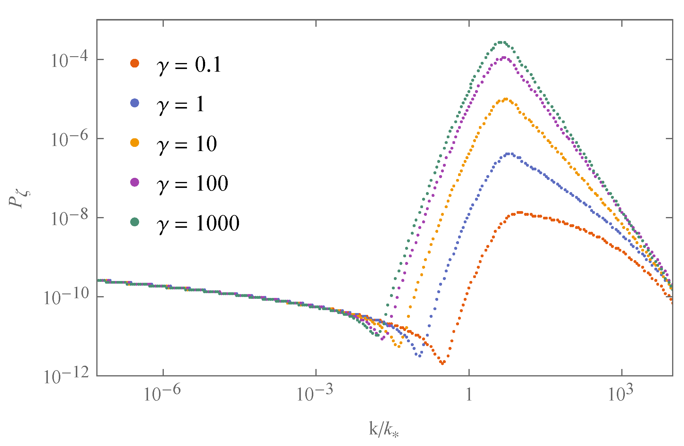
| 1 | 10 | 100 | 1000 | ||
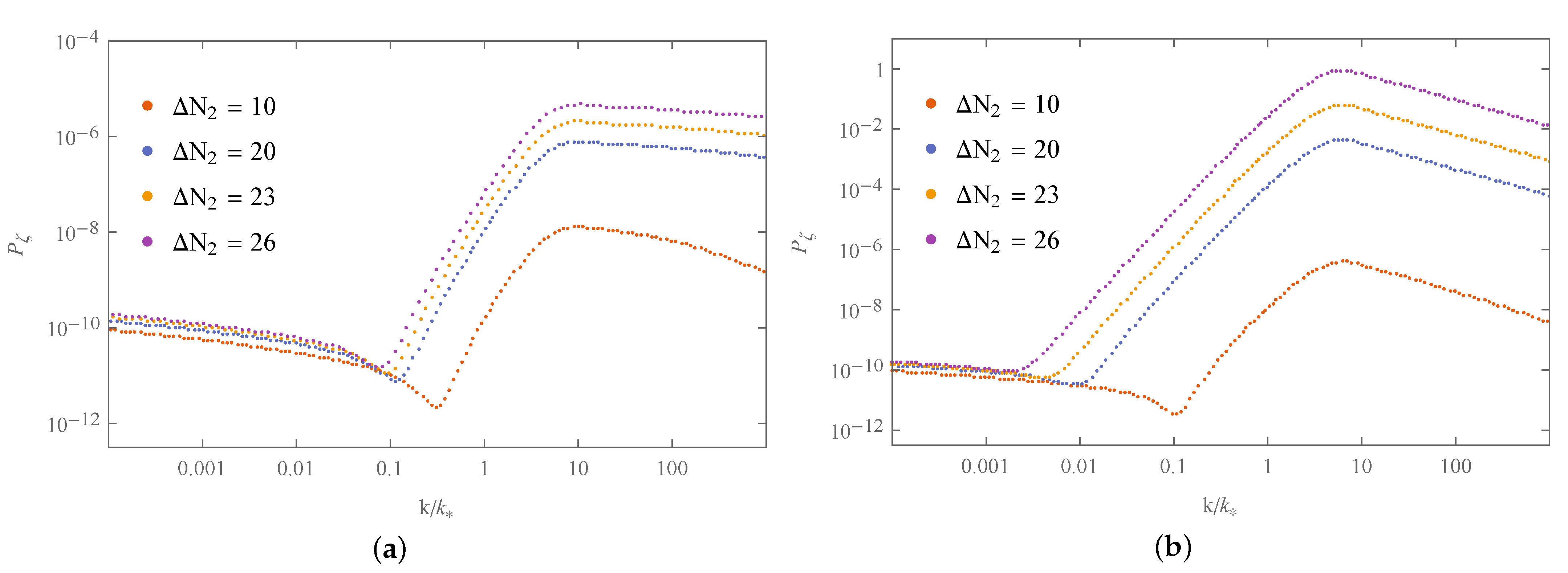
| 10 | 20 | 23 | 26 | |
|---|---|---|---|---|
| 10 | 20 | 23 | 26 | |
|---|---|---|---|---|
| , g | ||||
| 10 | 20 | 23 | 26 | 10 | 20 | 23 | 26 | |
|---|---|---|---|---|---|---|---|---|
| , g | ||||||||
| r | ||||||
|---|---|---|---|---|---|---|
| Case I | 0 | 20 | ||||
| Case II | 0 | 19 | ||||
| Case III | 0 | 20 |
Publisher’s Note: MDPI stays neutral with regard to jurisdictional claims in published maps and institutional affiliations. |
© 2021 by the author. Licensee MDPI, Basel, Switzerland. This article is an open access article distributed under the terms and conditions of the Creative Commons Attribution (CC BY) license (https://creativecommons.org/licenses/by/4.0/).
Share and Cite
Ketov, S.V. Multi-Field versus Single-Field in the Supergravity Models of Inflation and Primordial Black Holes. Universe 2021, 7, 115. https://doi.org/10.3390/universe7050115
Ketov SV. Multi-Field versus Single-Field in the Supergravity Models of Inflation and Primordial Black Holes. Universe. 2021; 7(5):115. https://doi.org/10.3390/universe7050115
Chicago/Turabian StyleKetov, Sergei V. 2021. "Multi-Field versus Single-Field in the Supergravity Models of Inflation and Primordial Black Holes" Universe 7, no. 5: 115. https://doi.org/10.3390/universe7050115
APA StyleKetov, S. V. (2021). Multi-Field versus Single-Field in the Supergravity Models of Inflation and Primordial Black Holes. Universe, 7(5), 115. https://doi.org/10.3390/universe7050115