Abstract
We study the size frequency distribution of the blocks located in the deeply fractured, geologically active Enceladus South Polar Terrain with the aim to suggest their formative mechanisms. Through the Cassini ISS images, we identify ~17,000 blocks with sizes ranging from ~25 m to 366 m, and located at different distances from the Damascus, Baghdad and Cairo Sulci. On all counts and for both Damascus and Baghdad cases, the power-law fitting curve has an index that is similar to the one obtained on the deeply fractured, actively sublimating Hathor cliff on comet 67P/Churyumov-Gerasimenko, where several non-dislodged blocks are observed. This suggests that as for 67P, sublimation and surface stresses favor similar fractures development in the Enceladus icy matrix, hence resulting in comparable block disaggregation. A steeper power-law index for Cairo counts may suggest a higher degree of fragmentation, which could be the result of localized, stronger tectonic disruption of lithospheric ice. Eventually, we show that the smallest blocks identified are located from tens of m to 20–25 km from the Sulci fissures, while the largest blocks are found closer to the tiger stripes. This result supports the ejection hypothesis mechanism as the possible source of blocks.
1. Introduction
Enceladus is a ~500 km-size icy moon of Saturn [1], orbiting at a distance of 3.94 Saturn radii from the planet. Its surface is dominated by pure water ice [2], heavily cratered in the northern latitudes as well as in its trailing and leading mid-latitude hemispheres. Through Voyager 1 and 2 km-scale images [3,4], it was assessed that Enceladus is characterized by different geological units, documenting a complex origin and evolution.
In 2005, the Cassini Imaging Science Subsystem—Narrow Angle Camera (ISS-NAC, [5]) acquired high-resolution images of the moon’s surface [6], revealing an almost craterless, fracture-dominated and geologically active province surrounding the South Pole of Enceladus, called the South Polar Terrain (SPT). Inside this unit (called csp, i.e., central south polar, surrounded by the southern curvilinear unit, called cl3, [7]), both cryovolcanic and tectonic activities are evident [7,8,9], with icy geysers emanating water vapor plumes from four, 100 km-long equally-spaced tension fractures [6], called “tiger stripes” (hereafter named TS), Figure 1.
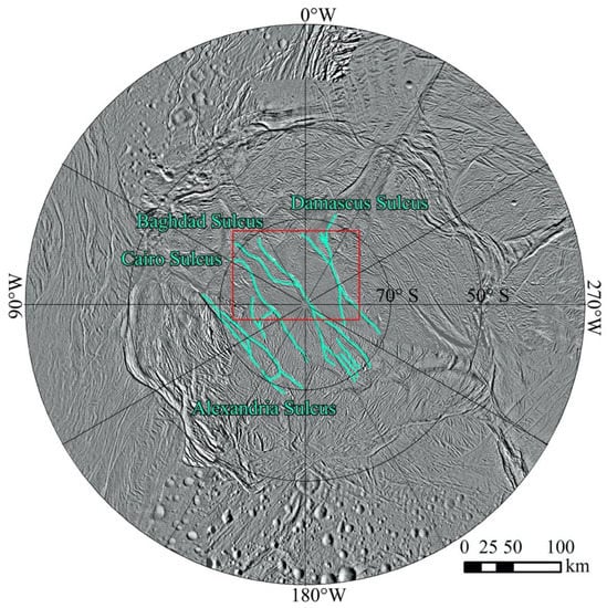
Figure 1.
Polar stereographic map of Enceladus southern hemisphere. The four main TS Damascus, Baghdad, Cairo and Alexandria Sulci are highlighted in light blue, following Crow-Willard and Pappalardo [7]. The red rectangle shows the location of our study area, presented in Figure 2.
Porco et al. [10] evidenced that the origin of such jets is strictly related to normal tensile stresses that open vertical pathways inside the TS (the fractures open and close from apocenter to pericenter, [11]), reaching the ocean that is located between 5 to 40 km underneath [12,13,14,15]. Through these conduits water vapor and liquid can reach the surface, hence depositing the latent heat they have [16,17].
In order to have higher-resolution views of the geyser vents and to study the TS rugged floors and their closest surroundings, three Enceladus close flybys have been performed by Cassini in the August-October 2008 timeframe, and in November 2009. The returned m-scale images have been unprecedented and led to the identification that the spacing of geysers is uniform along the three most active tiger stripes (Damascus, Bagdad and Cairo Sulci, [18]). In addition, the orientation of the observed jets is strongly correlated with the directions of the TS, crosscutting fractures or the orientation of local tectonic features [18].
The meter-to-decameter scale ISS-NAC images revealed also the presence of positive-relief icy blocks located in the SPT (hereafter called blocks), situated in close proximity to the TS. Martens et al. [1] focused on the spatial density of such features, showing that the variations in number density can be substantial over short spatial scale. Since impact cratering cannot be considered as the source of the SPT blocks, nor seismic disturbance or mass wasting, Martens et al. [1] suggested that sublimation processes, ballistic emplacement through geysers eruption and/or tectonic disruption of lithospheric ice can be the source of the blocks.
Besides the blocks spatial density, it is well established that the identification of the size-frequency distribution (SFD) of blocks/boulders and the corresponding curve fitting is a pivotal technique that can provide important hints to the formative and/or degradation processes of such features, as showed on the Moon [19,20,21,22], Mars [23,24,25,26,27], as well as on asteroids [28,29,30,31,32] and comets [33,34,35,36]. For this reason, we decided to expand the Martens et al. [1] work analyzing the size-distance relation between the blocks and the fractured Sulci, and obtaining the SFD of the identifiable blocks in the TS area (Figure 1), hence suggesting their generation processes.
The paper is structured as follows: after identifying and counting the blocks located in the Damascus-Baghdad-Cairo Sulci area, we study their SFD, applying a statistical method to evaluate if the data can be fitted by power-law curves. We then discuss the reliability of this approach and study in more detail the block SFD of the three TS, separately. We then discuss our results in the light of similar studies accomplished on other icy studied bodies.
2. Dataset and Methodology
In order to identify the icy blocks located in the Enceladus SPT, we downloaded the full Cassini ISS-NAC [5] imagery dataset presented in Table 1 of Martens et al. [1], and publicly available through the Planetary Data System (PDS) Archive (https://pds-rings.seti.org/saturn/, accessed on 20 June 2020). Out of the twenty images, we decided to focus on seven (Table 1). This choice was dictated by the fact that such images (i) are not dominated by large shadowed areas that commonly cover more than half of the observed surface, (ii) present a comparable spatial scale, hence favoring the identification of similar block sizes and (iii) cover the widest, almost contiguous area located inside the SPT (Figure 2). This aspect is of great importance since it allows to identify if there are any block SFD differences among the most active TS terrains. In addition to this dataset, we added the ISS-NAC image N1604167158 (indicated in italic in Table 1) that is not present in Martens et al. [1]. This was done to complement the N1597182533 coverage of Damascus Sulcus to the easternmost side. Despite the slightly lower resolution (31.9 m for N1604167158 vs. 25.3 m on N1597182533), this choice allowed a wider block identification, favored by similar illumination conditions.

Table 1.
Image ID, acquisition date and spatial scale of the Cassini ISS-NAC images used in this analysis.
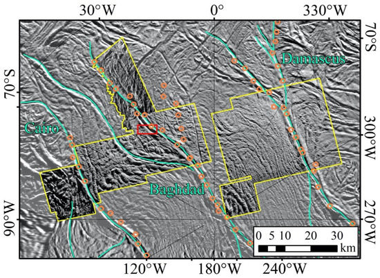
Figure 2.
The eight projected ISS-NAC images covering the region of interest between Damascus, Baghdad and Cairo Sulci (highlighted in light blue, following Crow-Willard and Pappalardo [7]). The yellow outline shows the full area covered by the dataset. On the left side of the saw-tooth yellow boundary, a bad signal-to-noise part of the image has been eliminated. The red rectangle shows the location of Figure 3, while the orange circles show the jets’ sources identified by Porco et al. [10].
As detailed in Martens et al. [1], we used the Integrated Software for Imagers and Spectrometers (ISIS) in order to convert the raw images into ISIS-readable data cubes, hence attaching all the required Navigation and Ancillary Information Facility (NAIF) SPICE kernels [37] information (mutual position of the target and the spacecraft, camera pointing, as well as spacecraft timing). This was accomplished to map all images into a polar stereographic projection, ready to be imported into the Environmental Systems Research Institute ArcGIS 10.5 software (hereafter ArcGIS).
Through ArcGIS, we then identified the blocks that are located on, or in close proximity to, the TS thanks to the presence of a nearby elongated shadow (Figure 3A). As commonly done by similar analyses performed on other bodies of the Solar System [26,38,39], once such features have been manually identified, we measured their position on the surface, assumed their shapes to be circumcircles (the maximum resolution of the images does not allow to outline them as polygons) and then calculated their diameter [40], Figure 3B. Finally, to derive the cumulative blocks SFD per km2, we computed the corresponding area of the studied surface.
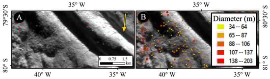
Figure 3.
Methodology used to identify the blocks located on Enceladus tiger stripes. (A) Subframe of the ISS-NAC N1597182500 image. The yellow arrow shows the direction of the solar irradiation. (B) The identified blocks are grouped in size (m).
Afterwards, it is possible to evaluate if the resulting SFD is fitted by a power-law or not [41,42]. To do that, we made use of the Clauset et al. [43] method to validate the existence of the power-law fitting model, which is characterized by the scaling parameter called . We highlight that the power-law index of the cumulative distribution we herafter refer to as “”, is related to the scaling parameter through the following equation: . The Clauset et al. [43] method also allows the identification of the completeness limit xmin, which is the threshold value above which the power-law exists. The estimation of xmin is done through the Kolmogorov-Smirnoff (KS) statistic and allows to find the value minimizing it. Afterwards, the parameter is determined through the maximum likelihood estimator (MLE). The uncertainty for both and xmin is then derived through a non-parametric bootstrap procedure that generates a large number of synthetic datasets from a power-law random generator and performs a number of KS tests to verify if the generated and observed data come from the same distribution. This technique returns a p-value that can be used to quantify the plausibility of the hypothesis. Considering the significance level of 0.10 [43], if the p-value is 0.1, then it is possible to conclude that any difference between the empirical data and the model can be explained with statistical fluctuations. On the contrary, if the p-value is <0.1, then the data set does not come from a power-law distribution, but instead, from a different one.
3. Results
Over the full study area (yellow outline in Figure 2) we identified 17,070 blocks (Figure 4). The resulting histogram of all counts is presented in Figure 5A. The diameter range of the counted blocks spans between ~25–30 m and 366 m, with the biggest block identified ~4000 m far from the Damascus Sulcus. As already presented in multiple works, e.g., [22,32], block sizes are only reasonably reliable for sizes larger than 3–4 pixels. Given that the lowest spatial scale of the full dataset is ~31 m, only the right tail of the distribution (with diameters larger than 125 m) can be considered meaningful to compute the main statistical properties. The mode of the resulting frequency distribution for diameters larger than 125 m is 133.8 m, the median is 145.3 m with a median absolute deviation (mad) of 21.7 m, while the mean value is 156.4 m, with a standard deviation of 34.9 m. The total considered area is 3296.1 km2 wide: we can therefore plot the unbinned cumulative number of blocks per km2 (Figure 5B) deriving values that span from 410−3/km2 at a diameter of 300 m, up to 510−1/km2 for sizes ~125 m.
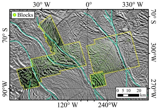
Figure 4.
The 17,070 blocks identified in the SPT between Damascus, Baghdad and Cairo Sulci.
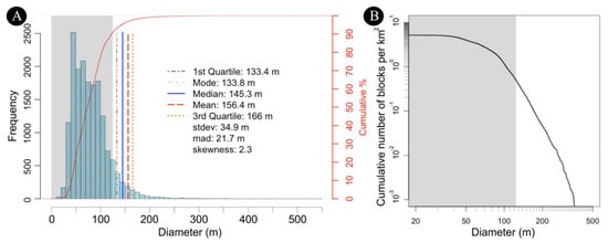
Figure 5.
(A) Frequency histogram of all blocks identified in the yellow area of Figure 4. The grey shadowed area shows the blocks that have been identified, but their diameter is smaller than 4 pixels. The main statistical properties of the right-skewed distribution are computed only for values 125 m. (B) Log-log plot showing the cumulative unbinned number of blocks per km2. As for A, the grey shadowed area shows all blocks <125 m.
By using the above mentioned Clauset et al. [43] methodology, we decided to test if the cumulative distribution function (CDF) can be fitted by a power-law or not. Through the KS statistic we identified that the completeness limit xmin for all counts is 149.8 m (with a total number of 688 blocks larger than xmin), while the value of the power-law index is −5.4 (Figure 6A). To evaluate the uncertainty for xmin and we generated 5000 synthetic datasets using the non-parametric bootstrap procedure. The scatter-plot of xmin against is presented in Figure 6B in order to evaluate how a change in xmin results in a different value for , while the frequency histograms of xmin and are indicated in Figure 6C,D. The resulting error of xmin is 16.2 m, while the one for is 0.37. As indicated in Figure 6A, the p-value obtained is 0.185. Since this value is 0.1, it is possible to affirm that (i) any difference between the empirical data and the model can be explained with statistical fluctuations, (ii) we cannot reject the power-law model for these data, and (iii) the data are consistent with a power-law.
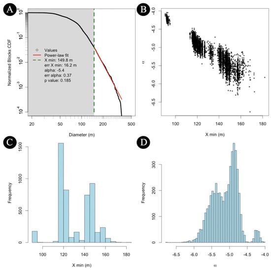
Figure 6.
(A) Normalized cumulative distribution function showing the obtained sizes, the power-law fitting curve and the xmin limit (the grey shadowed area is not considered by the fit). The total number of blocks larger than xmin and used for the fit is 688. (B) Scatter-plot of xmin against resulting from 5000 synthetic datasets. (C) Frequency histogram of xmin. (D) Frequency histogram of the power-law index .
In order to evaluate if there are any possible differences in cumulative size frequency distribution per km2 or power-law indices, we decided to split the full dataset of blocks into three main groups (Figure 7): (i) one belonging to the Damascus Sulcus, (ii) one characterized by the blocks situated in close proximity to the Baghdad Sulcus, while (iii) the last one surrounding the Cairo Sulcus. Even if the Baghdad Sulcus branches out in two parts on the studied area, we decided to consider the corresponding blocks as belonging to the same group since the tiger stripe has the same origin.
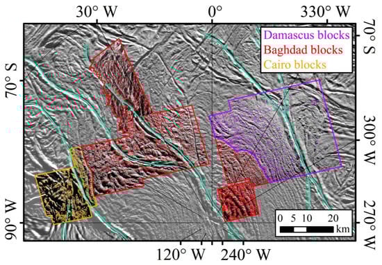
Figure 7.
The division of the study area into three different groups: the Damascus, Baghdad and Cairo blocks.
As done for the full dataset (Figure 5A), we plotted the histograms of the Damascus, Baghdad and Cairo Sulci blocks (Figure 8A,C,E), while we plotted the corresponding cumulative number of blocks per km2 in Figure 8B,D,F. The Damascus area (1208 km2) has a total number of 1838 counted blocks (the lowest spatial scale of the images used for the Damascus block identification is 31.9 m/pixel) and it is the one that shows the largest diameter range, between ~40 and 366 m (Figure 8A). The mode of the skewed distribution for all blocks 127 m (4 pixels) lies at 132.4 m, the median at 150.7 m (with a mad of 23.5 m), the mean is 162.0 m, and the standard deviation is 38.2 m. The cumulative number of blocks per km2 ranges from a minimum of 8.310−4/km2 at a size of 366 m to 5.110−1/km2 at 127 m (Figure 8B).
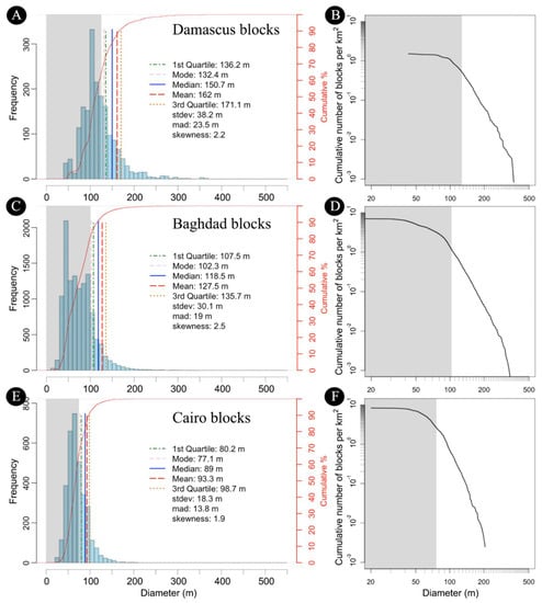
Figure 8.
(A,C,E) Frequency histogram of the sizes identified in the Damascus, Baghdad and Cairo areas. The grey shadowed area shows the blocks that have been identified, but their diameter is smaller than 4 pixels. The main statistical properties of the right-skewed distributions are computed only for values 4 pixels. (B,D,F) Log-log plots showing the cumulative unbinned number of blocks per km2 for the Damascus, Baghdad and Cairo area, respectively. As for (A,C,E), the grey shadowed area shows all blocks smaller than 127 m (Damascus), 101 m (Baghdad) and 74 m (Cairo).
Among the three considered areas, the Baghdad one is the widest with a total surface of 1685.1 km2. Out of the 11,883 blocks counted (the lowest spatial scale of the images used for the Baghdad block identification is 25.3 m/pixel), the largest one has a diameter of 343 m and it is located 1150 m far from the Baghdad left branch. The mode of the distribution of blocks 101 m is 102.3 m (Figure 8C), the median is 118.5 m with a mad of 19 m, while the mean lies at 127.5 m, with a standard deviation of 30.1 m. The cumulative number of blocks per km2 at the maximum identified size (~340 m) is 6.010−4/km2 and it is comparable to the Damascus one, while at 101 m size the cumulative number of blocks per km2 is 1.30/km2 (Figure 8D).
The third area, called Cairo, is 403 km2 wide and the total number of counted blocks is 3349 (the lowest spatial scale of the images used for the Cairo block identification is 18.4 m/pixel). The biggest block here identified has a diameter of 206 m (Figure 8E). The mode of the distribution of blocks larger than 4 pixels (~74 m) lies at 77.1 m, the median at 89.0 m (with a mad of 13.8 m), while the mean is 93.3 m, and the standard deviation is 18.3 m. The cumulative number of blocks per km2 is 2.510−3/km2 at the size of 206 m while it is 2.9/km2 at 74 m (Figure 8F).
In order to test if the cumulative distribution functions can be fitted by a power-law or not, we decided to apply the Clauset et al. [43] methodology also to the Damascus, Baghdad and Cairo separate counts. As done for the total counts’ analysis, we then evaluated the uncertainty for xmin and generating 5000 synthetic datasets using the non-parametric bootstrap procedure. The results are presented in Figure 9, Figure 10 and Figure 11, outlined with the same fashion of Figure 6.
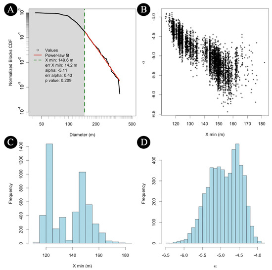
Figure 9.
The Damascus case study. (A) Normalized cumulative distribution function showing the obtained sizes, the power-law fitting curve and the xmin limit (the grey shadowed area is not considered by the fit). The total number of blocks larger than xmin and used for the fit is 327. (B) Scatter-plot of xmin against resulting from 5000 synthetic datasets. (C) Frequency histogram of xmin. (D) Frequency histogram of the power-law index .
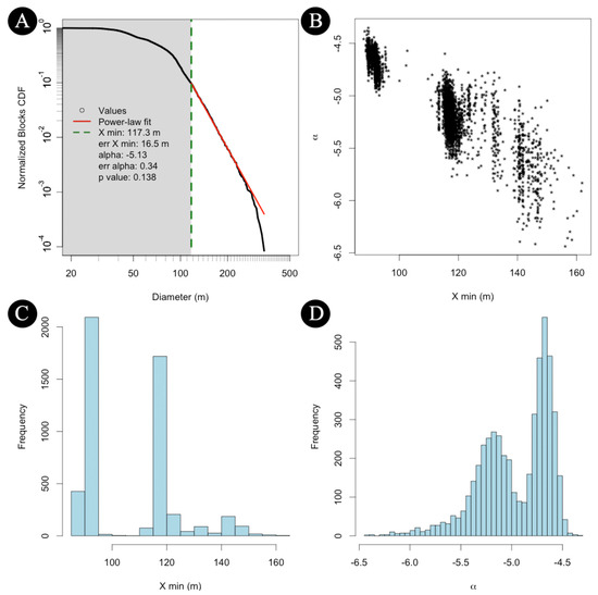
Figure 10.
The Baghdad case study. (A) Normalized cumulative distribution function showing the obtained sizes, the power-law fitting curve and the xmin limit (the grey shadowed area is not considered by the fit). The total number of blocks larger than xmin and used for the fit is 1156. (B) Scatter-plot of xmin against resulting from 5000 synthetic datasets. (C) Frequency histogram of xmin. (D) Frequency histogram of the power-law index .
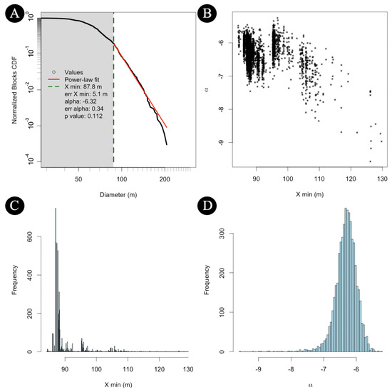
Figure 11.
The Cairo case study. (A) Normalized cumulative distribution function showing the obtained sizes, the power-law fitting curve and the xmin limit (the grey shadowed area is not considered by the fit). The total number of blocks larger than xmin and used for the fit is 659. (B) Scatter-plot of xmin against resulting from 5000 synthetic datasets. (C) Frequency histogram of xmin. (D) Frequency histogram of the power-law index .
For the Damascus case we obtained a xmin value of 149.6 14.2 m and a power-law index of −5.11 0.43. The resulting p-value is 0.21. The Clauset et al. [43] methodology applied on the Baghdad counts, instead, returned a xmin value of 117.3 16.5 m, a power-law index of −5.13 0.34 and a p-value of 0.14. Finally, for the Cairo case we obtained a xmin value of 87.8 5.1 m, a value of −6.32 0.34, and a p-value of 0.11.
We highlight that for all three cases the p-values obtained are 0.1, hence we can affirm that the use of the power-law curve fitting is meaningful for Damascus, Baghdad and Cairo counts, and any difference between the empirical data and the models are purely explainable with statistical fluctuations.
4. Discussion
Given the extremely complex geological setting of the SPT [7] and the ongoing multiple processes (cryovolcanic, tectonic, tidal and thermal) that are occurring in the TS area [6,7,8,9,11,17,18], no single formative process can be invoked to explain the formation, degradation and replenishment of the blocks observed on Enceladus south pole. Nevertheless, before describing which are the blocks’ originating processes that can be supported by our analysis, it is worth mentioning which are the ones that can be ruled out. As Martens et al. [1] extensively highlighted, impact cratering cannot be the considered as the driving mechanism originating such blocks, since almost no crater has been found in the SPT. Seismic disturbance or mass wasting events cannot be invoked either, because they would foresee disproportionately high concentrations of blocks in topographic lows, but the observed icy features appear on top of ridges, slopes and inside valleys (Figure 4 and Figure 7).
On the contrary, by taking into account the vapor density, the drag force, as well as the gravitational acceleration at the surface of Enceladus (0.11 m/s2), Martens et al. [1] evidenced that the ejection process occurring during cryovolcanic eruptions from the TS could be a supported block formative mechanism. It is difficult to conceive that wide enough cracks could let ~100 m size blocks pass, since to form such large nozzles both high stresses and strain rates would be needed [44]. However, Hansen et al. [45] indicated that Enceladus collimated jets could reach speeds of 1 km/s or higher, and assuming plume temperatures higher than 296 K, blocks with sizes ~100 m could be lifted and ejected [1].
To test the cryovolcanic eruptions as a possible block formation mechanism, for each of our identified blocks we measured the corresponding distance from the nearby TS (Figure 7). In this way we can therefore investigate if there is any block diameter versus TS distance trend, and whether the largest blocks appear closer to the ejection fissures. As presented in Figure 12, when the blocks with sizes smaller than the four pixels identification limit are excluded, it becomes evident that as distance from the TS fissure increases, the blocks’ sizes get smaller. Indeed, the smallest blocks (75 m to 130 m size) are present at different TS distance, from tens of m to maximum distances of 20–25 km. On the contrary, the largest blocks (100 s m wide) are generally found at much closer range. This result quantitively supports the ejection hypothesis previously advanced by Martens et al. [1], i.e., where larger blocks usually land closer to the ejection point.
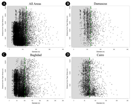
Figure 12.
Diameter versus TS distance plots obtained for all counts (A), for the Damascus blocks (B), for the Baghdad counts (C) and for the Cairo blocks (D). The vertical green dashed lines are the four pixels limit derived for each case, see Figure 5 and Figure 8. On all plots, the counts located inside the grey shadowed area are not considered because they are below the four pixels identification limit.
Since the blocks’ formation cannot be attributed to a single formative process, another mechanism that needs to be considered is the sublimation of ice in the SPT. Indeed, by modelling the ice sublimation in the 170–240 K temperature range (obtained in the TS area through CIRS data, [46]), Goguen et al. [47] evidenced that sublimation can erode m-scale layers of ice within weeks. Such process is particularly strong close to the geyser vents, i.e., where thermal emissions are concentrated, thermal gradients are larger and hence sublimation rates are higher, but it can still act on the full SPT over longer periods of time, disaggregating blocks from exposed, fractured ice. For this reason, the sublimation process can largely contribute to the evolution of blocks located on SPT. Such phenomenon has not been solely hypothesized on Enceladus [1], but also on another icy body, yet characterized by different size (4 km versus 500 km) and sublimation source (rapidly changing solar insolation versus tidal stress), such as comet 67P/Churyumov-Gerasimenko, herafter 67P.
Thanks to the high-resolution images acquired by the OSIRIS camera [48] onboard the ESA/Rosetta spacecraft, comet 67P is the only case of an icy surface where several boulders/blocks’ fields located on different morphological settings have been identified and analyzed. For instance, Pajola et al. [33] studied the cometary protruding blocks located in the heavily fractured, highly sublimating [49,50] Hathor cliff, which is a 900-m high, 1.8 km2 wide scarp located in 67P small lobe [51]. Besides gravity and tidal stresses, this location can be considered somehow geologically similar to the Enceladus SPT due to its ubiquitous fracture pattern and the active jets, hence allowing the comparison between the two bodies. By studying the Hathor non-dislodged blocks SFD in the 7–40 size range, Pajola et al. [33] derived a power-law index of −5.2 + 0.5/−0.6 (see Figure 11 and Figure 12 of Pajola et al. [33]), which has been attributed to both sublimation and fracturing processes. This value is similar to the one we obtained for the SPT full counts (Figure 6, = −5.4 0.4), as well as for the Damascus (Figure 9, = −5.1 0.4) and Baghdad case (Figure 10, = −5.1 0.3). Despite a larger block size range for Enceladus, similar power-law indices may suggest that sublimation and surface stresses favor similar fractures development in the icy matrix, hence resulting in comparable block disaggregation.
Instead, the Cairo blocks SFD is characterized by a steeper power-law index ( = −6.3 0.3) when compared to the Damascus and Baghdad case. As evidenced in Schröder et al. [32], even for several hundreds of boulders, a difference of 1 in the power-law index may arise simply by chance. This means that the Cairo SFD could still be comparable to the Damascus and Baghdad ones, in particular because the error bars are not small enough to argue this forcefully. Nevertheless, if the Cairo SFD is different from the other two, such steep power-law index could be indicative of a high degree of fragmentation [33]. A similar power-law index has been obtained on locations different from Hathor on comet 67P, and it is related to ceiling breakdown, rapid escape of high-pressure volatiles and consequent pit formation, with a resulting blocks’ field at its bottom [52,53]. Through the current imaging resolution, we have not identified an unusually higher density of pits inside Cairo, nor it appears to show more erupting vents, or jets (Figure 2, [10]), therefore we cannot invoke such formative mechanism for Cairo’s blocks. Such steep SFD may be alternatively related to a locally higher degree of tectonic disruption of lithospheric ice [1] that could be favored by thermal anomalies and ice crust thickness differences that appear to be prominent both inside the Sulci area, as well as at 30–50 km distance from the active SPT location [54]. The large localized thermal gradients may then result in a larger presence of smaller size blocks (hence affecting the steepness of the SFD), when compared to the largest ones. Nevertheless, since Cairo’s morphological setting shows no specific peculiarities with respect to Damascus or Baghdad TS (with the present resolution imagery dataset), this point remains to be justified.
Our results suggest that the comparison between Enceladus TS area and Hathor on 67P is intriguing, since it supports the hypothesis that at different size scales, the icy blocks observed on the two bodies could be the result of the coupled fracturing and sublimation activity. This analysis has been made possible because for both cases we have high enough resolution images to identify and measure the sizes of blocks/boulders on their surfaces, hence allowing to advance hypotheses on their formation.
5. Conclusions
Through the Cassini/ISS-NAC high-resolution images of the Enceladus Damascus-Baghdad-Cairo TS area, we have identified 17,070 blocks with sizes ranging from ~25–30 m to 366 m. Then, we identified the blocks SFD and its curve fitting to provide new insights into the formation and/or degradation processes characterizing these features. By using the Clauset et al. [43] methodology we derived that the TS blocks SFD can be fitted by a power-law curve, with a power-law of −5.4 0.4. The same methodology applied on the three TS separately studied returned a power-law index of −5.1 0.4 for the Damascus case, −5.1 0.3 for Baghdad TS, while a power-law index of −6.3 0.3 for the Cairo area. We explained these results considering that different processes concur in the formation and evolution of such blocks, in particular sublimation and cryovolcanic ejection mechanisms, as previously hypothesized by Martens et al. [1].
To support our findings, we compared our TS SFDs with comet 67P, the only other case of an icy surface where several boulders’ fields located on different morphological settings have been identified so far. In particular, the 67P Hathor cliff, where a ubiquitous fracture pattern with several departing jets have been observed, presents a similar SFD (−5.2 + 0.5/−0.6) to the Damascus and Baghdad ones. The sublimation and fracturing processes explaining the Hathor SFD can be applied also to the TS blocks’ SFD, suggesting that such mechanisms may favor similar fractures development in the icy matrix, resulting in comparable block disaggregation. For the Cairo case, the steeper power-law index may be indicative of a high degree of fragmentation that could be instead related to a locally higher degree of tectonic disruption of lithospheric ice favored by thermal anomalies and ice crust thickness differences [1], resulting in a larger presence of smaller size blocks. Nevertheless, since Cairo’s morphological setting shows no specific peculiarities with respect to Damascus or Baghdad TS, this different power-law index requires further investigation.
Afterwards, we also investigated the block diameter versus TS distance trend in order to test if the cryovolcanic ejection mechanism suggested by Martens et al. [1] can be a possible block formation process. From our counts, we identified that the smallest blocks (75 m to 130 m size) are present from tens of m to maximum distances of 20–25 km from the TS fissures, while the largest blocks (100s m wide) are generally found at much closer range. This result positively supports the vent eruption hypothesis, which foresees that larger blocks usually land closer to the ejection point.
Our findings support that sublimation and cryovolcanic eruptions could explain the formation and evolution of blocks located in the Enceladus SPT, but further higher-resolution data are required to test if such mechanisms could be invoked also for smaller sizes. Indeed, m- or cm-scale images are pivotal to largely advance our knowledge of the icy block/boulder SFD formation, as already done in the last decades [20,24,29,32] on different rocky bodies.
In this context, future space missions dedicated to icy worlds will be fundamental; in particular, the images that will be acquired by the JANUS camera [55] onboard the ESA/JUICE mission [56] and the EIS camera [57] of the NASA/Europa Clipper mission [58] will allow to compare and expand the presented study also to the icy surfaces of Europa, Ganymede and Callisto.
Author Contributions
Conceptualization, M.P.; methodology, M.P. and A.L.; software, M.P. and A.L.; validation, A.L., L.S. and G.C.; formal analysis, M.P., A.L. and L.S.; investigation, M.P., A.L. and L.S.; writing—original draft preparation, M.P., A.L. and G.C.; writing—review and editing, A.L., L.S., G.C.; visualization, M.P.; funding acquisition, G.C. and A.L. All authors have read and agreed to the published version of the manuscript.
Funding
This activity has been realized under the ASI-INAF contract 2018-25-HH.0.
Data Availability Statement
The blocks statistics presented in this paper are available upon request sent to the email address: maurizio.pajola@inaf.it.
Acknowledgments
This work is dedicated to all the victims of the COVID-19 and to the doctors who gave and are still giving their energy, time and lives during the ongoing pandemic. We thank Stefan Schröder, the two anonymous Referees and the Academic Editor for important and constructive comments that lead to a great improvement of the paper. We made use of the ArcGIS 10.5, R and Matlab softwares to perform the presented analysis. We also thank the Andraz-Livinnallongo del Col di Lana (Belluno-Italy) and the Casale (Vicenza-Italy) communities for providing us access to their wide Saturn and Jupiter icy satellites library.
Conflicts of Interest
The authors declare no conflict of interest.
References
- Martens, H.R.; Ingersoll, A.P.; Ewald, S.P.; Helfenstein, P.; Giese, B. Spatial distribution of ice blocks on Enceladus and implications for their origin and emplacement. Icarus 2015, 245, 162–176. [Google Scholar] [CrossRef]
- Verbiscer, A.J.; Peterson, D.E.; Skrutskie, M.F.; Cushing, M.; Helfenstein, P.; Nelson, M.J.; Smith, J.; Wilson, J.C. Near-infrared spectra of the leading and trailing hemispheres of Enceladus. Icarus 2006, 182, 211–223. [Google Scholar] [CrossRef]
- Smith, B.A.; Soderblom, L.; Beebe, R.; Boyce, J.; Briggs, G.; Bunker, A.; Collins, S.A.; Hansen, C.J.; Johnson, T.V.; Mitchell, J.L.; et al. Encounter with Saturn: Voyager 1 Imaging Science Results. Science 1981, 212, 163–191. [Google Scholar] [CrossRef]
- Smith, B.A.; Soderblom, L.; Batson, R.; Bridges, P.; Inge, J.; Masursky, H.; Shoemaker, E.; Beebe, R.; Boyce, J.; Briggs, G.; et al. A New Look at the Saturn System: The Voyager 2 Images. Science 1982, 215, 504–537. [Google Scholar] [CrossRef]
- Porco, C.C.; West, R.A.; Squyres, S.; McEwen, A.; Thomas, P.; Murray, C.D.; DelGenio, A.; Ingersoll, A.P.; Johnson, T.V.; Neukum, G.; et al. Cassini Imaging Science: Instrument Characteristics and Anticipated Scientific Investigations At Saturn. Space Sci. Rev. 2004, 115, 363–497. [Google Scholar] [CrossRef]
- Porco, C.C.; Helfenstein, P.; Thomas, P.C.; Ingersoll, A.P.; Wisdom, J.; West, R.; Neukum, G.; Denk, T.; Wagner, R.; Roatsch, T.; et al. Cassini Observes the Active South Pole of Enceladus. Science 2006, 311, 1393–1401. [Google Scholar] [CrossRef] [PubMed]
- Crow-Willard, E.N.; Pappalardo, R.T. Structural mapping of Enceladus and implications for formation of tectonized regions. J. Geophys. Res. Planets 2015, 120, 928–950. [Google Scholar] [CrossRef]
- Yin, A.; Pappalardo, R.T. Gravitational spreading, bookshelf faulting, and tectonic evolution of the South Polar Terrain of Saturn’s moon Enceladus. Icarus 2015, 260, 409–439. [Google Scholar] [CrossRef]
- Rossi, C.; Cianfarra, P.; Salvini, F.; Bourgeois, O.; Tobie, G. Tectonics of Enceladus’ South Pole: Block Rotation of the Tiger Stripes. J. Geophys. Res. Planets 2020, 125, 006471. [Google Scholar] [CrossRef]
- Porco, C.C.; DiNino, D.; Nimmo, F. How the geysers, tidal stresses, and thermal emission across the south polar terrain of enceladus are related. Astron. J. 2014, 148. [Google Scholar] [CrossRef]
- Hedman, M.M.; Gosmeyer, C.M.; Nicholson, P.D.; Sotin, C.; Brown, R.H.; Clark, R.N.; Baines, K.H.; Buratti, B.J.; Showalter, M.R. An observed correlation between plume activity and tidal stresses on Enceladus. Nat. Cell Biol. 2013, 500, 182–184. [Google Scholar] [CrossRef]
- Iess, L.; Stevenson, D.J.; Parisi, M.; Hemingway, D.; Jacobson, R.A.; Lunine, J.I.; Nimmo, F.; Armstrong, J.W.; Asmar, S.W.; Ducci, M.; et al. The Gravity Field and Interior Structure of Enceladus. Science 2014, 344, 78–80. [Google Scholar] [CrossRef]
- Čadek, O.; Tobie, G.; Van Hoolst, T.; Massé, M.; Choblet, G.; Lefèvre, A.; Mitri, G.; Baland, R.-M.; Běhounková, M.; Bourgeois, O.; et al. Enceladus’s internal ocean and ice shell constrained from Cassini gravity, shape, and libration data. Geophys. Res. Lett. 2016, 43, 5653–5660. [Google Scholar] [CrossRef]
- Lucchetti, A.; Pozzobon, R.; Mazzarini, F.; Cremonese, G.; Massironi, M. Brittle ice shell thickness of Enceladus from fracture distribution analysis. Icarus 2017, 297, 252–264. [Google Scholar] [CrossRef]
- Hemingway, D.; Iess, L.; Tadjeddine, R.; Tobie, G. The Interior of Enceladus. In Enceladus and the Icy Moons of Saturn; University of Arizona: Tucson, AZ, USA, 2018; pp. 57–77. [Google Scholar]
- Spencer, J.R. Cassini Encounters Enceladus: Background and the Discovery of a South Polar Hot Spot. Science 2006, 311, 1401–1405. [Google Scholar] [CrossRef]
- Spitale, J.N.; Porco, C.C. Association of the jets of Enceladus with the warmest regions on its south-polar fractures. Nat. Cell Biol. 2007, 449, 695–697. [Google Scholar] [CrossRef] [PubMed]
- Helfenstein, P.; Porco, C.C. Enceladus’ geysers: Relation to geological features. Astron. J. 2015, 150. [Google Scholar] [CrossRef]
- Cintala, M.J.; McBride, K.M. Block Distributions on the Lunar Surface: A Comparison between Measurements Obtained from Surface and Orbital Photography. In NASA Technical Memorandum 104804. 1995. Available online: https://www.lpi.usra.edu/lunar/documents/NASA_TM_104804_Lunar_blocks.pdf (accessed on 13 July 2020).
- Bart, G.D.; Melosh, H. Distributions of boulders ejected from lunar craters. Icarus 2010, 209, 337–357. [Google Scholar] [CrossRef]
- Krishna, N.; Kumar, P.S. Impact spallation processes on the Moon: A case study from the size and shape analysis of ejecta boulders and secondary craters of Censorinus crater. Icarus 2016, 264, 274–299. [Google Scholar] [CrossRef]
- Pajola, M.; Pozzobon, R.; Lucchetti, A.; Rossato, S.; Baratti, E.; Galluzzi, V.; Cremonese, G. Abundance and size-frequency distribution of boulders in Linné crater’s ejecta (Moon). Planet. Space Sci. 2019, 165, 99–109. [Google Scholar] [CrossRef]
- Garvin, J.B.; Mouginis-Mark, P.J.; Head, J.W. Characterization of rock populations on planetary surfaces: Techniques and a preliminary analysis of Mars and Venus. Earth Moon Planets 1981, 24, 355–387. [Google Scholar] [CrossRef]
- Grant, J.A.; Wilson, S.A.; Ruff, S.W.; Golombek, M.P.; Koestler, D.L. Distribution of rocks on the Gusev Plains and on Husband Hill, Mars. Geophys. Res. Lett. 2006, 33, 16202. [Google Scholar] [CrossRef]
- Golombek, M.P.; Huertas, A.; Marlow, J.; McGrane, B.; Klein, C.; Martinez, M.; Arvidson, R.E.; Heet, T.; Barry, L.; Seelos, K.; et al. Size-frequency distributions of rocks on the northern plains of Mars with special reference to Phoenix landing surfaces. J. Geophys. Res. Space Phys. 2008, 113. [Google Scholar] [CrossRef]
- Pajola, M.; Rossato, S.; Baratti, E.; Pozzobon, R.; Quantin, C.; Carter, J.; Thollot, P. Boulder abundances and size-frequency distributions on Oxia Planum-Mars: Scientific implications for the 2020 ESA ExoMars rover. Icarus 2017, 296, 73–90. [Google Scholar] [CrossRef]
- Mastropietro, M.; Pajola, M.; Cremonese, G.; Munaretto, G.; Lucchetti, A. Boulder Analysis on the Oxia Planum ExoMars 2022 Rover Landing Site: Scientific and Engineering Perspectives. Sol. Syst. Res. 2020, 54, 504–519. [Google Scholar] [CrossRef]
- Geissler, P.; Petit, J.-M.; Durda, D.D.; Greenberg, R.; Bottke, W.; Nolan, M.; Moore, J. Erosion and Ejecta Reaccretion on 243 Ida and Its Moon. Icarus 1996, 120, 140–157. [Google Scholar] [CrossRef]
- Thomas, P.C.; Veverka, J.; Robinson, M.S.; Murchie, S. Shoemaker crater as the source of most ejecta blocks on the asteroid 433 Eros. Nat. Cell Biol. 2001, 413, 394–396. [Google Scholar] [CrossRef]
- Mazrouei, S.; Daly, M.; Barnouin, O.; Ernst, C.; DeSouza, I. Block distributions on Itokawa. Icarus 2014, 229, 181–189. [Google Scholar] [CrossRef]
- DellaGiustina, D.N.; The OSIRIS-REx Team; Emery, J.P.; Golish, D.R.; Rozitis, B.; Bennett, C.A.; Burke, K.N.; Ballouz, R.-L.; Becker, K.J.; Christensen, P.R.; et al. Properties of rubble-pile asteroid (101955) Bennu from OSIRIS-REx imaging and thermal analysis. Nat. Astron. 2019, 3, 341–351. [Google Scholar] [CrossRef]
- Schröder, S.E.; Carsenty, U.; Hauber, E.; Schulzeck, F.; Raymond, C.A.; Russell, C.T. The Boulder Population of Asteroid 4 Vesta: Size-Frequency Distribution and Survival Time. Earth Space Sci. 2021, 8, 000941. [Google Scholar] [CrossRef]
- Pajola, M.; Vincent, J.-B.; Güttler, C.; Lee, J.-C.; Bertini, I.; Massironi, M.; Simioni, E.; Marzari, F.; Giacomini, L.; Lucchetti, A.; et al. Size-frequency distribution of boulders ≥7 m on comet 67P/Churyumov-Gerasimenko. Astron. Astrophys. 2015, 583, A37. [Google Scholar] [CrossRef]
- Mottola, S.; Arnold, G.; Grothues, H.-G.; Jaumann, R.; Michaelis, H.; Neukum, G.; Bibring, J.-P.; Schroder, S.E.; Hamm, M.; Otto, K.A.; et al. The structure of the regolith on 67P/Churyumov-Gerasimenko from ROLIS descent imaging. Science 2015, 349, aab0232. [Google Scholar] [CrossRef] [PubMed]
- Pajola, M.; Lucchetti, A.; Vincent, J.; Oklay, N.; El-Maarry, M.; Bertini, I.; Naletto, G.; Lazzarin, M.; Massironi, M.; Sierks, H. The southern hemisphere of 67P/Churyumov-Gerasimenko: Analysis of the pre-perihelion size-frequency distribution of boulders >7 m. Astron. Astrophys. 2016, 592, 2. [Google Scholar] [CrossRef][Green Version]
- Pajola, M.; Lucchetti, A.; Bertini, I.; Marzari, F.; A’Hearn, M.F.; La Forgia, F.; Lazzarin, M.; Naletto, G.; Barbieri, C. Size-frequency distribution of boulders ≥10 m on comet 103P/Hartley 2. Astron. Astrophys. 2015, 585, A85. [Google Scholar] [CrossRef]
- Acton, C.H. Ancillary data services of NASA’s Navigation and Ancillary Information Facility. Planet. Space Sci. 1996, 44, 65–70. [Google Scholar] [CrossRef]
- Michikami, T.; Nakamura, A.M.; Hirata, N.; Gaskell, R.W.; Nakamura, R.; Honda, T.; Honda, C.; Hiraoka, K.; Saito, J.; Demura, H.; et al. Size-frequency statistics of boulders on global surface of asteroid 25143 Itokawa. Earth Planets Space 2008, 60, 13–20. [Google Scholar] [CrossRef]
- Küppers, M.; Moissl, R.; Vincent, J.-B.; Besse, S.; Hviid, S.F.; Carry, B.; Grieger, B.; Sierks, H.; Keller, H.U.; Marchi, S. Boulders on Lutetia. Planet. Space Sci. 2012, 66, 71–78. [Google Scholar] [CrossRef]
- Pajola, M.; Höfner, S.; Vincent, J.-B.; Oklay, N.; Scholten, F.; Preusker, F.; Mottola, S.; Naletto, G.; Fornasier, S.; Lowry, S.; et al. The pristine interior of comet 67P revealed by the combined Aswan outburst and cliff collapse. Nat. Astron. 2017, 1, 0092. [Google Scholar] [CrossRef]
- Mohajeri, N.; Gudmundsson, A. Entropies and Scaling Exponents of Street and Fracture Networks. Entropy 2012, 14, 800–833. [Google Scholar] [CrossRef]
- Lucchetti, A.; Rossi, C.; Mazzarini, F.; Pajola, M.; Pozzobon, R.; Massironi, M.; Cremonese, G. Equatorial grooves distribution on Ganymede: Length and self-similar clustering analysis. Planet. Space Sci. 2021, 195, 105140. [Google Scholar] [CrossRef]
- Clauset, A.; Shalizi, C.R.; Newman, M.E.J. Power-Law Distributions in Empirical Data. SIAM Rev. 2009, 51, 661–703. [Google Scholar] [CrossRef]
- Crawford, G.D.; Stevenson, D.J. Gas-driven water volcanism and the resurfacing of Europa. Icarus 1988, 73, 66–79. [Google Scholar] [CrossRef]
- Hansen, C.J.; Shemansky, D.E.; Esposito, L.W.; Stewart, A.I.F.; Lewis, B.R.; Colwell, J.E.; Hendrix, A.R.; West, R.A.; Waite, J.H.; Teolis, B.; et al. The composition and structure of the Enceladus plume. Geophys. Res. Lett. 2011, 38. [Google Scholar] [CrossRef]
- Abramov, O.; Spencer, J. Endogenic heat from Enceladus’ south polar fractures: New observations, and models of conductive surface heating. Icarus 2009, 199, 189–196. [Google Scholar] [CrossRef]
- Goguen, J.D.; Buratti, B.J.; Brown, R.H.; Clark, R.N.; Nicholson, P.D.; Hedman, M.M.; Howell, R.R.; Sotin, C.; Cruikshank, D.P.; Baines, K.H.; et al. The temperature and width of an active fissure on Enceladus measured with Cassini VIMS during the 14 April 2012 South Pole flyover. Icarus 2013, 226, 1128–1137. [Google Scholar] [CrossRef]
- Keller, H.U.; Barbieri, C.; Lamy, P.; Rickman, H.; Rodrigo, R.; Wenzel, K.-P.; Sierks, H.; A’Hearn, M.F.; Angrilli, F.; Angulo, M.; et al. OSIRIS—The Scientific Camera System Onboard Rosetta. Space Sci. Rev. 2007, 128, 433–506. [Google Scholar] [CrossRef]
- Sierks, H.; Barbieri, C.; Lamy, P.L.; Rodrigo, R.; Koschny, D.; Rickman, H.; Keller, H.U.; Agarwal, J.; A’Hearn, M.F.; Angrilli, F.; et al. On the nucleus structure and activity of comet 67P/Churyumov-Gerasimenko. Science 2015, 347, aaa1044. [Google Scholar] [CrossRef]
- Alí-Lagoa, V.; Delbo, M.; Libourel, G. Rapid temperature changes and the early activity on comet 67P/Churyumov–Gerasimenko. Astrophys. J. 2015, 810, L22. [Google Scholar] [CrossRef]
- Thomas, N.; Sierks, H.; Barbieri, C.; Lamy, P.L.; Rodrigo, R.; Rickman, H.; Koschny, D.; Keller, H.U.; Agarwal, J.; A’Hearn, M.F.; et al. The morphological diversity of comet 67P/Churyumov-Gerasimenko. Science 2015, 347, aaa0440. [Google Scholar] [CrossRef]
- Pajola, M.; Oklay, N.; La Forgia, F.; Giacomini, L.; Massironi, M.; Bertini, I.; El-Maarry, M.R.; Marzari, F.; Preusker, F.; Scholten, F.; et al. Aswan site on comet 67P/Churyumov-Gerasimenko: Morphology, boulder evolution, and spectrophotometry. Astron. Astrophys. 2016, 592, A69. [Google Scholar] [CrossRef]
- Pajola, M.; Lee, J.-C.; Oklay, N.; Hviid, S.F.; Penasa, L.; Mottola, S.; Shi, X.; Fornasier, S.; Davidsson, B.; Giacomini, L.; et al. Multidisciplinary analysis of the Hapi region located on Comet 67P/Churyumov–Gerasimenko. Mon. Not. R. Astron. Soc. 2019, 485, 2139–2154. [Google Scholar] [CrossRef]
- Le Gall, A.; Leyrat, C.; Janssen, M.A.; Choblet, G.; Tobie, G.; Bourgeois, O.; Lucas, A.; Sotin, C.; Howett, C.; Kirk, R.; et al. Thermally anomalous features in the subsurface of Enceladus’s south polar terrain. Nat. Astron. 2017, 1, 0063. [Google Scholar] [CrossRef]
- Palumbo, P.; Jaumann, R.; Cremonese, G.; Hoffmann, H.; Debei, S.; Della Corte, V.; Holland, A.; Lara, L.M.; Castro, J.M.; Herranz, M.; et al. JANUS: The Visible Camera Onboard the ESA JUICE Mission to the Jovian System. 45th LPSC Meeting. Abstract #2094. 2014. Available online: https://elib.dlr.de/90175/1/2094.pdf (accessed on 4 January 2021).
- Grasset, O.; Dougherty, M.; Coustenis, A.; Bunce, E.; Erd, C.; Titov, D.; Blanc, M.; Coates, A.; Drossart, P.; Fletcher, L.; et al. JUpiter ICy moons Explorer (JUICE): An ESA mission to orbit Ganymede and to characterise the Jupiter system. Planet. Space Sci. 2013, 78, 1–21. [Google Scholar] [CrossRef]
- Turtle, E.P.; McEwen, A.S.; Bland, M.; Collins, G.C.; Daubar, I.J.; Ernst, C.M.; Fletcher, L.; Hansen, C.J.; Hawkins, S.E.; Hayes, A.G.; et al. The Europa Imaging System (EIS): High-Resolution, 3-D Insight into Europa’s Geology, Ice Shell, and Potential for Current Activity. EPSC-DPS Joint Meeting 2019. Volume 13, EPSC-DPS2019–832-2. 2019. Available online: https://meetingorganizer.copernicus.org/EPSC-DPS2019/EPSC-DPS2019-832-2.pdf (accessed on 4 January 2021).
- Pappalardo, R.T.; Senske, D.; Korth, H.; Klima, R.; Vance, S.; Craft, K. The Europa Clipper Mission: Exploring the Habitability of a Unique Icy World. EPSC 2017 Abstracts. 2017, Volume 11–304. 2017. Available online: https://meetingorganizer.copernicus.org/EPSC2017/EPSC2017-304.pdf (accessed on 4 January 2021).


Publisher’s Note: MDPI stays neutral with regard to jurisdictional claims in published maps and institutional affiliations. |
© 2021 by the authors. Licensee MDPI, Basel, Switzerland. This article is an open access article distributed under the terms and conditions of the Creative Commons Attribution (CC BY) license (https://creativecommons.org/licenses/by/4.0/).