Nonperturbative Quantization Approach for QED on the Hopf Bundle  ^†

Abstract

We consider the Dirac equation and Maxwell’s electrodynamics in $\mathbb{R}\times S^3$ spacetime, where a three-dimensional sphere is the Hopf bundle $S^3\to S^2$. In both cases, discrete spectra of classical solutions are obtained. Based on the solutions obtained, the quantization of free, noninteracting Dirac and Maxwell fields is carried out. The method of nonperturbative quantization of interacting Dirac and Maxwell fields is suggested. The corresponding operator equations and the infinite set of the Schwinger–Dyson equations for Green’s functions is written down. We write a simplified set of equations describing some physical situations to illustrate the suggested scheme of nonperturbative quantization. Additionally, we discuss the properties of quantum states and operators of interacting fields.

1. Introduction

Quantum electrodynamics (QED) and the electroweak theory are very successful in explaining quantum phenomena for electromagnetic and weak interactions. Their predictions agree with experimental data to great precision. This progress was achieved, despite the fact that the calculations are perturbative and one needs to involve, for example, a renormalization procedure. R. Feynman called this procedure “sweeping the garbage under the rug”. L. Landau et al. [1] wrote on this subject: “Although at present there exist methods to remove these singularities (regularization), which clearly lead to correct results, such method of action has the artificial nature. The singularities arise in the theory due to the pointlike interaction described by delta functions (operators of interacting fields are taken at one point)”. In References [2,3,4], he and his co-authors study this question trying to remove such singularities in QED.

Attempts to use this technique for strong interactions do not lead to a full success and, in gravity, they are unsuccessful. This suggests that, at present, we do not clearly understand the nature of quantization. It is reasonable to assume that there should exist some well-defined mathematical procedure of quantization that can be applied to any field theory. This cannot be a perturbative technique used, for instance, in QED, since it leads to nonrenormalizable theories. This suggests that the aforementioned procedure of quantization, applicable to any field theory, must be nonperturbative. It should be pointed out here that the nonperturbative quantization technique was perhaps first suggested by W. Heisenberg in Reference [5], where he proposed an idea that an electron can be described by a nonperturbatively quantized nonlinear spinor field.

Taking all of this into account, it is of great interest to construct nonperturbative QED for some simple case in order to compare perturbative and nonperturbative QED. It would allow for one to understand the physical essence of such phenomena, like the renormalization, convergence of the Feynman integral, etc. One can assume that such a possibility may arise in constructing QED on some compact manifold, since, in this case, the spectra of eigenvalues of the Dirac and Maxwell equations will presumably be discrete. This would permit one to replace the Fourier integral in a general solution by a summation over quantum numbers that give the number of the eigenvalues. In doing so, Dirac delta functions would be replaced by the Kronecker symbols, and all of the calculations would be simplified; this would presumably permit one to construct nonperturbative QED. Simultaneously, it would be possible to construct perturbative QED according to conventional methods, but taking into account the compactness of three-dimensional space. After that, there would appear the possibility of comparison of perturbative and nonperturbative quantum theories.

In the present paper, we find a discrete spectrum of classical solutions describing noninteracting Dirac and Maxwell fields in a spacetime with a spatial cross-section in the form of the Hopf bundle. Subsequently, we use the spectra obtained to quantize the Dirac equation and Maxwell’s electrodynamics. Finally, we suggest a scheme of nonperturbative quantization of coupled Dirac and Maxwell fields.

The paper is organized, as follows. In Section 2, we give the Lagrangian, field equations, and $\mathfrak{Ansatze}$ for the Dirac and Maxwell equations on the Hopf bundle. Using them, we obtain classical solutions to the Dirac (Section 3) and Maxwell (Section 4) equations separately. In Section 5, we quantize free, noninteracting fields and obtain expressions for the corresponding propagators. In Section 6, we carry out the nonperturbative quantization on the Hopf bundle. Finally, in Section 7, we discuss the results that were obtained and list the important problems in nonperturbative quantum field theory.

2. Classical Electrodynamics Plus the Dirac Equation

In this section, we consider classical electrodynamics coupled to spinors obeying the Dirac equation in $\mathbb{R}\times S^3$ spacetime with a spatial cross-section in the form of the Hopf bundle $S^3\to S^2$. One can say that a relativistic quantum theory of an electron interacting with an electromagnetic field and living on the the Hopf bundle is under consideration.

Here, we closely follow Reference [6]. Consider Dirac–Maxwell theory with the source of electromagnetic field taken in the form of a massless Dirac field. The corresponding Lagrangian can be chosen in the form (hereafter, we work in units where $\hslash =c=1$)

$$L=\frac{i}{2}\left(\overline{\psi }{\gamma }^{\mu }{\psi }_{;\mu }-{\overline{\psi }}_{;\mu }{\gamma }^{\mu }\psi \right)-\frac{1}{4}{F}_{\mu \nu }{F}^{\mu \nu }$$

(1)

with the covariant derivative ${\psi }_{;\mu }\equiv \left[{\partial }_{\mu }+1/8{\omega }_{ab\mu }\left({\gamma }^a{\gamma }^b-{\gamma }^b{\gamma }^a\right)-ie{A}_{\mu }\right]\psi$, where ${\gamma }^a$ are the Dirac matrices in flat space (below, we use the spinor representation of the matrices); $a,b$ and $\mu ,\nu$ are tetrad and spacetime indices, respectively; $F_{\mu \nu }={\partial }_{\mu }{A}_{\nu }-{\partial }_{\nu }{A}_{\mu }$ is the electromagnetic field tensor; $A_{\mu }$ are four-potentials of the electromagnetic field; and, e is a charge in Maxwell theory. In turn, the Dirac matrices in curved space, ${\gamma }^{\mu }=e_a^{\phantom{a}\mu }{\gamma }^a$, are derived while using the tetrad $e_a^{\phantom{a}\mu }$, and ${\omega }_{ab\mu }$ is the spin connection [for its definition, see Reference [7], formula (7.135)].

Varying the corresponding action with the Lagrangian (1), one can derive the following set of equations:

$$\begin{array}{cc}\hfill i{\gamma }^{\mu }{\psi }_{;\mu }=& 0,\hfill \end{array}$$

(2)

$$\begin{array}{cc}\hfill \frac{1}{\sqrt{-g}}\frac{\partial }{\partial x^{\nu }}\left(\sqrt{-g}{F}^{\mu \nu }\right)=& -4\pi j^{\mu },\hfill \end{array}$$

(3)

where g is the determinant of the metric tensor and $j^{\mu }=e\overline{\psi }{\gamma }^{\mu }\psi$ is the four-current.

The above equations will be solved in $\mathbb{R}\times S^3$ spacetime with the Hopf coordinates $\chi ,\theta ,\phi$ on a sphere $S^3$ with the metric

$$d{s}^2=d{t}^2-\frac{r^2}{4}\left[{\left(d\chi -cos\theta d\phi \right)}^2+d{\theta }^2+{sin}^2\theta d{\phi }^2\right]=d{t}^2-r^{2}d{S}_3^2,$$

(4)

where $d{S}_3^2$ is the Hopf metric on the unit $S^3$ sphere; r is a constant; amd. $0\le \chi ,\phi \le 2\pi$ and $0\le \theta \le \pi$.

To solve Equations (2) and (3), we employ the following $\mathfrak{Ansatze}$ for the spinor and electromagnetic fields:

$$\begin{array}{cc}\hfill {\psi }_{nm}& =e^{-i{\Omega }t}{e}^{in\chi }{e}^{im\phi }\left(\begin{array}{c}{{\Theta }}_1\left(\theta \right)\\ {{\Theta }}_2\left(\theta \right)\\ 0\\ 0\end{array}\right),\hfill \end{array}$$

(5)

$$\begin{array}{cc}\hfill A_{\mu }& =\left\{\varphi \left(\theta \right),r\rho \left(\theta \right),0,r\lambda \left(\theta \right)\right\},\hfill \end{array}$$

(6)

where m and n are integers. The spinor can transform under a rotation through an angle $2\pi$ as

$${\psi }_{mn}(\chi +2\pi ,\theta ,\phi +2\pi )={\psi }_{mn}(\chi ,\theta ,\phi ).$$

Subsequently, because of the presence of the factors $e^{in\chi }$ and $e^{im\phi }$ in Equation (5), the spinors ${\psi }_{mn}$ and ${\psi }_{pq}$ with different pairs of indices $(m,n)$ and $(p,q)$ are orthogonal.

To solve the equations, we use the tetrad

$$e_{\phantom{a}\mu }^a=\left(\begin{array}{cccc}1& 0& 0& 0\\ 0& \frac{r}{2}& 0& -\frac{r}{2}cos\theta \\ 0& 0& \frac{r}{2}& 0\\ 0& 0& 0& \frac{r}{2}sin\theta \end{array}\right)$$

coming from the metric (4).

On substitution of the $\mathfrak{Ansatze}$ (5) and (6) in Equations (2) and (3), we have

$$\begin{array}{cc}\hfill & {{\Theta }}_1^{\prime }+{{\Theta }}_1\left(\frac{cot\theta }{2}+n+er\rho \right)+\hfill \end{array}$$

$$\begin{array}{cc}\hfill & {{\Theta }}_2\left(\frac{1}{4}-\frac{r{\Omega }}{2}-ncot\theta -\frac{m}{sin\theta }-er\rho cot\theta -\frac{er\lambda }{sin\theta }+\frac{er}{2}\varphi \right)=0,\hfill \\ \hfill & {{\Theta }}_2^{\prime }+{{\Theta }}_2\left(\frac{cot\theta }{2}-n-er\rho \right)+\hfill \end{array}$$

(7)

$$\begin{array}{cc}\hfill & {{\Theta }}_1\left(-\frac{1}{4}+\frac{r{\Omega }}{2}-ncot\theta -\frac{m}{sin\theta }-er\rho cot\theta -\frac{er\lambda }{sin\theta }-\frac{er}{2}\varphi \right)=0,\hfill \end{array}$$

(8)

$$\begin{array}{cc}\hfill & \frac{1}{sin\theta }{\left(sin\theta {\varphi }^{\prime }\right)}^{\prime }={\varphi }^{″}+cot\theta {\varphi }^{\prime }=-\frac{e{r}^2}{4}\left({{\Theta }}_1^2+{{\Theta }}_2^2\right),\hfill \\ \hfill & {\left(\frac{{\rho }^{\prime }}{sin\theta }\right)}^{\prime }+{\left(cot\theta {\lambda }^{\prime }\right)}^{\prime }=\frac{{\rho }^{\prime \prime }}{sin\theta }-\frac{cot\theta }{sin\theta }{\rho }^{\prime }+cot\theta {\lambda }^{″}-\frac{{\lambda }^{\prime }}{{sin}^2\theta }=\hfill \end{array}$$

(9)

$$\begin{array}{cc}\hfill & \frac{e{r}^2}{8}\left[cos\theta \left({{\Theta }}_1^2-{{\Theta }}_2^2\right)+2sin\theta {{\Theta }}_1{{\Theta }}_2\right],\hfill \end{array}$$

(10)

$$\begin{array}{cc}\hfill & {\left(\frac{{\lambda }^{\prime }}{sin\theta }\right)}^{\prime }+{\left(cot\theta {\rho }^{\prime }\right)}^{\prime }=\frac{{\lambda }^{\prime \prime }}{sin\theta }-\frac{cot\theta }{sin\theta }{\lambda }^{\prime }+cot\theta {\rho }^{″}-\frac{{\rho }^{\prime }}{{sin}^2\theta }=\frac{e{r}^2}{8}\left({{\Theta }}_1^2-{{\Theta }}_2^2\right),\hfill \end{array}$$

(11)

where the prime denotes differentiation with respect to $\theta$. Notice that the set of Equations (7)–(11) must be solved as an eigenvalue problem for ${\Omega }$ with the eigenfunctions ${{\Theta }}_{1,2}$.

3. Classical Vacuum Solutions to the Dirac Equation

In this section we consider the case of "frozen” electric and magnetic fields with zero scalar and vector potentials, $\varphi =\rho =\lambda =0$. In this case, the parent Dirac Equations (7) and (8) take the form

$$\begin{array}{cc}\hfill {{\Theta }}_1^{\prime }+{{\Theta }}_1\left(\frac{cot\theta }{2}+n\right)+{{\Theta }}_2\left(\tilde{{\Omega }}-ncot\theta -\frac{m}{sin\theta }\right)& =0,\hfill \end{array}$$

(12)

$$\begin{array}{cc}\hfill {{\Theta }}_2^{\prime }+{{\Theta }}_2\left(\frac{cot\theta }{2}-n\right)+{{\Theta }}_1\left(-\tilde{{\Omega }}-ncot\theta -\frac{m}{sin\theta }\right)& =0,\hfill \end{array}$$

(13)

where $\tilde{{\Omega }}=\frac{1}{4}-\frac{r{\Omega }}{2}$. These equations are symmetric under the replacements ${{\Theta }}_1\to {{\Theta }}_2,{{\Theta }}_2\to -{{\Theta }}_1,n\to -n,m\to -m$. Introducing new functions

$${{\Sigma }}_1=\frac{{{\Theta }}_1+{{\Theta }}_2}{2},{{\Sigma }}_2=\frac{{{\Theta }}_1-{{\Theta }}_2}{2},$$

(14)

Equations (12) and (13) can be rewritten as

$$\begin{array}{cc}\hfill {{\Sigma }}_1^{\prime }+{{\Sigma }}_1\left(\frac{1}{2}cot\theta -ncot\theta -\frac{m}{sin\theta }\right)+{{\Sigma }}_2\left(n-\tilde{{\Omega }}\right)& =0,\hfill \end{array}$$

(15)

$$\begin{array}{cc}\hfill {{\Sigma }}_2^{\prime }+{{\Sigma }}_2\left(\frac{1}{2}cot\theta +ncot\theta +\frac{m}{sin\theta }\right)+{{\Sigma }}_1\left(n+\tilde{{\Omega }}\right)& =0,\hfill \end{array}$$

(16)

which are, in turn, symmetric under the replacements ${{\Sigma }}_2\to -{{\Sigma }}_1,{{\Sigma }}_1\to {{\Sigma }}_2,n\to -n,m\to -m.$ Upon finding ${{\Sigma }}_2$ from Equation (15),

$${{\Sigma }}_2=-\frac{{{\Sigma }}_1^{\prime }+{{\Sigma }}_1\left(\frac{1}{2}cot\theta -ncot\theta -\frac{m}{sin\theta }\right)}{n-\tilde{{\Omega }}},$$

(17)

and substituting it in (16), we get a second-order differential equation for the function ${{\Sigma }}_1$,

$${{\Sigma }}_1^{″}+cot\theta {{\Sigma }}_1^{\prime }-{{\Sigma }}_1\frac{\frac{1}{4}+n^2+m^2-n+\left(2mn-m\right)cos\theta +\frac{1-4{\tilde{{\Omega }}}^2}{4}{sin}^2\theta }{{sin}^2\theta }=0.$$

(18)

Similarly, for the function ${{\Sigma }}_2$, one can obtain the following equation:

$${{\Sigma }}_2^{″}+cot\theta {{\Sigma }}_2^{\prime }-{{\Sigma }}_2\frac{\frac{1}{4}+n^2+m^2+n+\left(2mn+m\right)cos\theta +\frac{1-4{\tilde{{\Omega }}}^2}{4}{sin}^2\theta }{{sin}^2\theta }=0.$$

(19)

Here, it should be noted that Equation (19) can be obtained from Equation (18) on simply replacing $m,n\to -m,-n$.

Equation (18) must be regarded as an eigenvalue problem for the parameter $\tilde{{\Omega }}$. This equation has the following general solution containing two linearly independent solutions:

$$\begin{array}{cc}\hfill {{\Sigma }}_1=& c_1{\left(1-cos\theta \right)}^{\alpha /2}{\left(1+cos\theta \right)}^{\beta /2}{}_2{F}_1\left(n-\tilde{{\Omega }},n+\tilde{{\Omega }};n+m+\frac{1}{2};\frac{1-cos\theta }{2}\right)\hfill \\ \hfill & +c_2{\left(1-cos\theta \right)}^{-\alpha /2}{\left(1+cos\theta \right)}^{\beta /2}\hfill \\ \hfill & {}_2{F}_1\left(-m-\tilde{{\Omega }}+\frac{1}{2},-m+\tilde{{\Omega }}+\frac{1}{2};-n-m+\frac{3}{2};\frac{1-cos\theta }{2}\right)\hfill \end{array}$$

(20)

with

$$\alpha =n+m-\frac{1}{2},\beta =n-m-\frac{1}{2}.$$

(21)

Substituting Equation (20) in Equation (17), we have

$$\begin{array}{cc}\hfill {{\Sigma }}_2=& -c_1\frac{n+\tilde{{\Omega }}}{2n+2m+1}{\left(1-cos\theta \right)}^{(\alpha +1)/2}{\left(1+cos\theta \right)}^{(\beta +1)/2}\hfill \\ \hfill & {}_2{F}_1\left(n+1-\tilde{{\Omega }},n+1+\tilde{{\Omega }};n+m+\frac{3}{2};\frac{1-cos\theta }{2}\right)\hfill \\ \hfill & +c_2\left\{\frac{{(m-\frac{1}{2})}^2-{\tilde{{\Omega }}}^2}{(2m+2n-3)(n-\tilde{{\Omega }})}{\left(1-cos\theta \right)}^{(1-\alpha )/2}{\left(1+cos\theta \right)}^{(\beta +1)/2}\right.\hfill \\ \hfill & \times {}_2{F}_1\left(-m-\tilde{{\Omega }}+\frac{3}{2},-m+\tilde{{\Omega }}+\frac{3}{2};-m-n+\frac{5}{2};\frac{1-cos\theta }{2}\right)\hfill \\ \hfill & +\frac{n+m-1/2}{(n-\tilde{{\Omega }})}{\left(1-cos\theta \right)}^{-\alpha /2}{\left(1+cos\theta \right)}^{1+\beta /2}\hfill \\ \hfill & \left.{}_2{F}_1\left(-m-\tilde{{\Omega }}+\frac{1}{2},-m+\tilde{{\Omega }}+\frac{1}{2};-m-n+\frac{3}{2};\frac{1-cos\theta }{2}\right)\right\}.\hfill \end{array}$$

(22)

It is known that the hypergeometric function ${}_2{F}_1(a,b;c;x)$ is regular at the points $x=0,1$ if either a or b is a negative integer. In our case, this has the result that, for the first independent solution in Equations (20) and (22), we have the quantization condition for the parameter $\tilde{{\Omega }}$,

$${\tilde{{\Omega }}}_{nl}=\pm (n+l),\mathrm{where}l=0,1,\dots$$

(23)

In this case, the hypergeometric function ${}_2{F}_1(a,b;c;x)={}_2{F}_1(b,a;c;x)$ is equal to the Jacobi polynomials

$$P_l^{\left(\gamma ,\delta \right)}\left(x\right)=\frac{{\left(\gamma +1\right)}_l}{l!}{}_2{F}_1\left(-l,1+\gamma +\delta +l;\gamma +1;\frac{1-x}{2}\right),$$

(24)

where ${\left(\gamma +1\right)}_l$ is the Pochhammer symbol. In our case, this gives the following values of the parameters $\gamma ,\delta$ and the variable x:

$$x=cos\theta ,\gamma =\alpha =n+m-\frac{1}{2},\delta =\beta =n-m-\frac{1}{2},l=-n\mp \tilde{{\Omega }}.$$

Thus, the first independent solution can be recast in the form

$$\begin{array}{cc}\hfill {{\Sigma }}_{1,nml}=& c_1\frac{l!}{{\left(\alpha +1\right)}_l}{\left(1-cos\theta \right)}^{\alpha /2}{\left(1+cos\theta \right)}^{\beta /2}{P}_l^{\left(\alpha ,\beta \right)}\left(cos\theta \right),\hfill \\ \hfill {{\Sigma }}_{2,nml}=& -c_1\frac{n+\tilde{{\Omega }}}{2n+2m+1}\frac{l!}{{\left(\alpha +1\right)}_l}{\left(1-cos\theta \right)}^{(\alpha +1)/2}{\left(1+cos\theta \right)}^{(\beta +1)/2}\hfill \end{array}$$

(25)

$$\begin{array}{cc}\hfill & P_{l-1}^{\left(\alpha +1,\beta +1\right)}\left(cos\theta \right),\hfill \end{array}$$

(26)

where the parameters $\alpha$ and $\beta$ are given by the expressions Equation (21). In order to ensure the regularity of the factors ${\left(1-cos\theta \right)}^{\alpha /2}$ and ${\left(1+cos\theta \right)}^{\beta /2}$, it is necessary that $\alpha ⩾0,\beta ⩾0$; this results in the following restrictions being imposed upon the integers n and m:

$$n⩾1,\left|m\right|⩽n-\frac{1}{2}.$$

(27)

The functions ${{\Sigma }}_{1,nmp}$ with different p and the functions ${{\Sigma }}_{2,nmp}$ are orthogonal:

$$\begin{gathered} \begin{array}{cc}\hfill \underset{0}{\overset{\pi }{\int }}sin\theta {{\Sigma }}_{1,nmp}{{\Sigma }}_{1,nmq}d\theta & =-c_1^2{\left[\frac{1}{{\left(\alpha +1\right)}_p}\frac{2^{\alpha +\beta +1}}{2p+\alpha +\beta +1}\frac{{\Gamma }(p+\alpha +1){\Gamma }(p+\beta +1)}{{\Gamma }(p+\alpha +\beta +1)}\right]}^2{\delta }_{pq}\hfill \\ \\ \hfill & =A_{nmp}{\delta }_{pq},\hfill \end{array} \end{gathered}$$

(28)

$$\begin{gathered} \begin{array}{cc}\hfill \underset{0}{\overset{\pi }{\int }}sin\theta {{\Sigma }}_{2,nmp}{{\Sigma }}_{2,nmq}d\theta & =-c_1^2{\left[\frac{1}{{\left(\alpha +2\right)}_p}\frac{2^{\alpha +\beta +3}}{2p+\alpha +\beta +3}\frac{{\Gamma }(p+\alpha +2){\Gamma }(p+\beta +2)}{{\Gamma }(p+\alpha +\beta +3)}\right]}^2{\delta }_{pq}\hfill \\ \\ \hfill \\ \hfill & =B_{nmp}{\delta }_{pq}.\hfill \end{array} \end{gathered}$$

(29)

Their orthogonality follows from the orthogonality condition for the Jacobi polynomials,

$$\underset{-1}{\overset{1}{\int }}{\left(1-x\right)}^{\rho }{\left(1+x\right)}^{\sigma }{P}_p^{\left(\rho ,\sigma \right)}\left(x\right)P_q^{\left(\rho ,\sigma \right)}\left(x\right)dx={\delta }_{pq},$$

where $\rho =\beta ,\sigma =\alpha$ for Equation (28) or $\rho =(\beta +1),\sigma =(\alpha +1)$ for Equation (29) and $x=-cos\theta$. The functions ${{\Sigma }}_{1,nmp}$ and ${{\Sigma }}_{2,nmp}$ are not orthogonal to each other.

Using the solutions (25) and (26), one can obtain the functions

$$\begin{array}{cc}\hfill {{\Theta }}_{1,nml}=& c_1\frac{l!}{{\left(\alpha +1\right)}_l}{\left(1-cos\theta \right)}^{\alpha /2}{\left(1+cos\theta \right)}^{\beta /2}\hfill \end{array}$$

$$\begin{array}{cc}\hfill & \left[P_l^{\left(\alpha ,\beta \right)}\left(cos\theta \right)-\frac{n+{\tilde{{\Omega }}}_{nl}}{2n+2m+1}sin\theta P_{l-1}^{\left(\alpha +1,\beta +1\right)}\left(cos\theta \right)\right],\hfill \\ \hfill {{\Theta }}_{2,nml}=& c_1\frac{l!}{{\left(\alpha +1\right)}_l}{\left(1-cos\theta \right)}^{\alpha /2}{\left(1+cos\theta \right)}^{\beta /2}\hfill \end{array}$$

(30)

$$\begin{array}{cc}\hfill & \left[P_l^{\left(\alpha ,\beta \right)}\left(cos\theta \right)+\frac{n+{\tilde{{\Omega }}}_{nl}}{2n+2m+1}sin\theta P_{l-1}^{\left(\alpha +1,\beta +1\right)}\left(cos\theta \right)\right]\hfill \end{array}$$

(31)

Consider the orthogonality of the corresponding spinors,

$${\psi }_{nml}=e^{-i{{\Omega }}_{nl}t}{e}^{in\chi }{e}^{im\phi }\left(\begin{array}{c}{{\Theta }}_{1,nml}\\ {{\Theta }}_{2,nml}\end{array}\right)={\psi }_{+1/2,nml}+{\psi }_{-1/2,nml},$$

(32)

where ${\psi }_{\pm ,nml}$ are:

$$\begin{array}{cc}\hfill {\psi }_{+,nml}=& {\tilde{c}}_1{e}^{-i{{\Omega }}_{nl}t}{e}^{in\chi }{e}^{im\phi }{\left(1-cos\theta \right)}^{\alpha /2}{\left(1+cos\theta \right)}^{\beta /2}{P}_l^{\left(\alpha ,\beta \right)}\left(cos\theta \right)\left(\begin{array}{c}1\\ 1\end{array}\right),\hfill \\ \hfill {\psi }_{-,nml}=& {\tilde{c}}_1\frac{n+{\tilde{{\Omega }}}_{nl}}{2n+2m+1}{e}^{-i{{\Omega }}_{nl}t}{e}^{in\chi }{e}^{im\phi }{\left(1-cos\theta \right)}^{(\alpha +1)/2}{\left(1+cos\theta \right)}^{(\beta +1)/2}\hfill \end{array}$$

(33)

$$\begin{array}{cc}\hfill & P_{l-1}^{\left(\alpha +1,\beta +1\right)}\left(cos\theta \right)\left(\begin{array}{c}-1\\ 1\end{array}\right).\hfill \end{array}$$

(34)

According to the remarks made after Equations (13) and (16), the following spinor is also the solution:

$${\tilde{\psi }}_{nml}=e^{-i{{\Omega }}_{-nl}t}{e}^{-in\chi }{e}^{-im\phi }\left(\begin{array}{c}{{\Theta }}_{2,nml}\\ -{{\Theta }}_{1,nml}\end{array}\right).$$

(35)

Notice that, in Reference [8], the solutions to the Dirac equation have also been found, but using the standard coordinates on a three-dimensional sphere. The results obtained here correspond to the results of Reference [8] in the sense that, in both cases, the energy levels are discrete; correspondingly, the solutions form a discrete spectrum.

Hereafter, we drop for brevity the zeroth components of the spinor, i.e., we consider Weyl spinors. The orthogonality condition is

$$\begin{array}{cc}\hfill 〈{\psi }_{nml},{\psi }_{pqr}〉=& \int \sqrt{\gamma }{\psi }_{nml}^{†}{\psi }_{pqr}dV=4{\pi }^2{\delta }_{np}{\delta }_{mq}\underset{0}{\overset{\pi }{\int }}sin\theta \left({{\Theta }}_{1,nml}{{\Theta }}_{1,pqr}+{{\Theta }}_{2,pqr}{{\Theta }}_{2,pqr}\right)d\theta \hfill \\ \hfill & =8{\pi }^2\left(A_{nml}+B_{nml}\right){\delta }_{np}{\delta }_{mq}{\delta }_{lq}=1,\hfill \end{array}$$

where $dV=sin\theta d\theta d\chi d\phi$ and we took the orthogonality of both the functions $e^{in\chi }$ with different integers n and of the functions $e^{im\chi }$ with different integers m into account; the normalization constant $c_1$ is chosen from this condition using the values of $A_{nml}$ and $B_{nml}$ from Equations (28) and (29).

Thus, the spinors (32) and (35) form the complete basis set on a three-dimensional sphere in the Hopf coordinates. It is important that this basis is numbered by integers, in contrast to Minkowski space, where the complete basis set is created by plain waves and it is numbered by real numbers. This essential distinction follows directly from the fact that a three-dimensional sphere $S^3$ is a compact space, in contrast to Minkowski space, which, in turn, is a noncompact space.

4. Classical Vacuum Solutions to the Maxwell Equations

In this section, we consider classical solutions with the “frozen” spinor field $\psi =0$. The four-potential $A_{\mu }$ for the Maxwell Equations (3) can be written in the form

$$A_{\mu }=e^{i\left(\frac{\omega }{r}t+p\chi +q\phi \right)}\left\{\varphi \left(\theta \right),r\rho \left(\theta \right),0,r\lambda \left(\theta \right)\right\},$$

(36)

where we have chosen the gauge $A_{\theta }=0$, and $p,q$ are integers. Using this potential, the Maxwell equations yield

$$\begin{array}{ccc}\hfill & {\varphi }^{″}+cot\theta {\varphi }^{\prime }-\frac{p^2+q^2+2pqcos\theta }{{sin}^2\theta }\varphi +\lambda \omega \frac{pcos\theta +q}{{sin}^2\theta }\hfill & +\rho \omega \frac{p+qcos\theta }{{sin}^2\theta }=0,\hfill \end{array}$$

(37)

$$\begin{array}{ccc}\hfill & {\rho }^{″}-cot\theta {\rho }^{\prime }+cos\theta {\lambda }^{″}-\frac{{\lambda }^{\prime }}{sin\theta }+\rho \left(\frac{{\omega }^2}{4}-q^2\right)+\lambda \left(\frac{1}{4}{\omega }^{2}cos\theta +pq\right)\hfill & -\varphi \frac{\omega \left(p+qcos\theta \right)}{4}=0,\hfill \end{array}$$

(38)

$$\begin{array}{cc}\hfill & \frac{1}{4}\omega {sin}^2\theta {\varphi }^{\prime }-{\lambda }^{\prime }\left(pcos\theta +q\right)-{\rho }^{\prime }\left(p+qcos\theta \right)=0,\hfill \end{array}$$

(39)

$$\begin{array}{ccc}\hfill & {\lambda }^{″}-cot\theta {\lambda }^{\prime }+cos\theta {\rho }^{″}-\frac{{\rho }^{\prime }}{sin\theta }+\lambda \left(\frac{{\omega }^2}{4}-p^2\right)+\rho \left(\frac{1}{4}{\omega }^{2}cos\theta +pq\right)\hfill & -\varphi \frac{\omega \left(q+pcos\theta \right)}{4}=0.\hfill \end{array}$$

(40)

This set of equations must be regarded as an eigenvalue problem with the eigenfunctions ${\varphi }_{pqn},{\rho }_{pqn},{\lambda }_{pqn}$ and the eigenvalue ${\omega }_{pqn}$, where the integer n numbers the eigenvalues of $\omega$ for the fixed values of the integers p and q.

This set of equations has the following discrete symmetries:

$$\begin{array}{cc}\hfill {\varphi }_{pqn}& ={\varphi }_{qpn},{\lambda }_{pqn}={\rho }_{qpn},{\rho }_{pqn}={\lambda }_{qpn},\hfill \end{array}$$

(41)

$$\begin{array}{cc}\hfill p& \to -p,q\to -q,\omega \to -\omega .\hfill \end{array}$$

(42)

Below, we consider regular solutions, as well as singular solutions that are supported by a pointlike charge and a current located at the points $\theta =0,\pi$.

4.1. Regular Solutions

Deriving an analytic solution to the set of Equations (37)–(40) runs into great difficulty. Therefore, in this subsection, we first find numerical solutions and then show that there are analytic solutions for some particular values of the numbers $p,q$ and of the functions $\varphi ,\rho$, and $\lambda$.

4.1.1. Numerical Solutions

It is necessary to assign the values of the functions and their derivatives at the point $\theta \ll 1$ in order to perform numerical computations. To do this, let us seek a solution in the form

$$\varphi ={\varphi }_0{\theta }^{\alpha }+\cdots ,\lambda ={\lambda }_0{\theta }^{\beta }+\cdots ,{\rho }_0={\rho }_0{\theta }^{\beta }+\cdots .$$

Subsequently, Equation (39) yields the following restriction on the parameters ${\varphi }_0,{\lambda }_0$, and ${\rho }_0$:

$${\varphi }_0=\frac{4(2+\alpha )}{\omega }\left({\lambda }_0+{\rho }_0\right)$$

with $\alpha =p+q$ and $\beta =2+\alpha$.

Figure 1 and Figure 2 show the results of numerical calculations of Equations (37)–(40) for the case of $p=0$ and $q=1$. These solutions are of interest, because they are vacuum, since Equations (37)–(40) do not contain the electric charge and current densities. Nevertheless, nontrivial (i.e., nonzero) solutions are present. This is because, in the case under consideration, the electric and magnetic fields live on a compact space, which enables the nontrivial fields to exist in vacuum.

The numerical solutions that were obtained for different p and q permit us to assume that solutions also apparently exist for all pairs of p and q, and they are regular for $p+q⩾0$. Thus, we can conclude that the set of Equations (37)–(40) apparently has a discrete spectrum of solutions

$${\left(A_{\mu }\right)}_{pqn}=e^{i\left(\frac{{\omega }_{pqn}}{r}t+p\chi +q\phi \right)}\left\{{\varphi }_{pqn},r{\rho }_{pqn},0,r{\lambda }_{pqn}\right\}=e^{i\left(\frac{{\omega }_{pqn}}{r}t+p\chi +q\phi \right)}{\left({\tilde{A}}_{\mu }\right)}_{pqn}.$$

(43)

According to the property of symmetry (42), there also exists the solution

$${\left(A_{\mu }\right)}_{pqn}=e^{-i\left(\frac{{\omega }_{pqn}}{r}t+p\chi +q\phi \right)}{\left({\tilde{A}}_{\mu }\right)}_{pqn}.$$

4.1.2. The Case of $p=q=\varphi =0,\rho =\lambda$

Here, it is possible to find an analytic solution. In this case, the Maxwell Equations (37)–(40) reduce to one equation

$${\lambda }^{″}-\frac{{\lambda }^{\prime }}{sin\theta }+\frac{{\omega }^2}{4}\lambda =0,$$

whose solution is

$$\lambda =\frac{c_1}{2}\left(cos\theta -1\right){}_2{F}_1\left(1-\frac{\omega }{2},1+\frac{\omega }{2};2;\frac{1-cos\theta }{2}\right),$$

where ${}_2{F}_1$ is the hypergeometric function. This solution is regular for the following eigenvalues of $\omega$:

$${\omega }_n=\pm 2n,$$

where n is integer.

4.1.3. The Case of $p=q$

Making use of the substitution $(\rho ,\lambda )\to \frac{\omega }{8p}(\tilde{\rho },\tilde{\lambda })$, Equations (37)–(40) can be rewritten as

$$\begin{array}{cc}\hfill & {\varphi }^{″}+cot\theta {\varphi }^{\prime }-\frac{p^2+q^2+2pqcos\theta }{{sin}^2\theta }\varphi +\tilde{\lambda }\frac{{\omega }^2}{8}\frac{cos\theta +\frac{q}{p}}{{sin}^2\theta }+\tilde{\rho }\frac{{\omega }^2}{8}\frac{1+\frac{q}{p}cos\theta }{{sin}^2\theta }=0,\hfill \\ \hfill & {\tilde{\rho }}^{″}-cot\theta {\tilde{\rho }}^{\prime }+cos\theta {\tilde{\lambda }}^{″}-\frac{{\tilde{\lambda }}^{\prime }}{sin\theta }+\tilde{\rho }\left(\frac{{\omega }^2}{4}-q^2\right)+\tilde{\lambda }\left(\frac{1}{4}{\omega }^{2}cos\theta +pq\right)\hfill \\ \hfill & -2\varphi p^2\left(1+\frac{q}{p}cos\theta \right)=0,\hfill \\ \hfill & {sin}^2\theta {\varphi }^{\prime }-{\tilde{\lambda }}^{\prime }\frac{cos\theta +\frac{q}{p}}{2}-{\tilde{\rho }}^{\prime }\frac{1+\frac{q}{p}cos\theta }{2}=0,\hfill \\ \hfill & {\tilde{\lambda }}^{″}-cot\theta {\tilde{\lambda }}^{\prime }+cos\theta {\tilde{\rho }}^{″}-\frac{{\tilde{\rho }}^{\prime }}{sin\theta }+\tilde{\lambda }\left(\frac{{\omega }^2}{4}-p^2\right)+\tilde{\rho }\left(\frac{1}{4}{\omega }^{2}cos\theta +pq\right)\hfill \\ \hfill & -2\varphi p^2\left(cos\theta +\frac{q}{p}\right)=0.\hfill \end{array}$$

Consider the particular case of $q=p$. In this case $\tilde{\lambda }\left(\theta \right)=\tilde{\rho }\left(\theta \right)$, and the Maxwell equations take the form

$$\begin{array}{cc}\hfill {\varphi }^{″}+cot\theta {\varphi }^{\prime }-p^2\frac{\varphi }{{sin}^2\left(\frac{\theta }{2}\right)}+\frac{{\omega }^2}{8}\frac{\tilde{\rho }}{{sin}^2\left(\frac{\theta }{2}\right)}& =0,\hfill \end{array}$$

(44)

$$\begin{array}{cc}\hfill {\tilde{\rho }}^{″}-\frac{{\tilde{\rho }}^{\prime }}{sin\theta }+\frac{{\omega }^2}{4}\tilde{\rho }-2p^2\varphi & =0,\hfill \end{array}$$

(45)

$$\begin{array}{cc}\hfill {\tilde{\rho }}^{\prime }+(cos\theta -1){\varphi }^{\prime }& =0.\hfill \end{array}$$

(46)

Expressing from Equation (45)

$$\varphi =\frac{{\tilde{\rho }}^{\prime \prime }-\frac{{\tilde{\rho }}^{\prime }}{sin\theta }+\frac{{\omega }^2}{4}\tilde{\rho }}{2p^2}$$

(47)

and substituting it in Equation (46), we have

$${sin}^2\theta {\tilde{\rho }}^{‴}-sin\theta {\tilde{\rho }}^{″}+{\tilde{\rho }}^{\prime }\left[\frac{{\omega }^2}{4}{sin}^2\theta +\left(1-2p^2\right)cos\theta -2p^2\right]=0.$$

Its solution for ${\tilde{\rho }}^{\prime }$ gives

$$\begin{array}{cc}\hfill {\tilde{\rho }}^{\prime }=& c_1{(1-cos\theta )}^{p+\frac{1}{2}}{(1+cos\theta )}^{-\frac{1}{2}}{}_2{F}_1\left(p-\frac{\omega }{2},p+\frac{\omega }{2};1+2p;\frac{1-cos\theta }{2}\right)\hfill \\ \hfill & +c_2{(1-cos\theta )}^{-p+\frac{1}{2}}{(1+cos\theta )}^{-\frac{1}{2}}{}_2{F}_1\left(-p-\frac{\omega }{2},-p+\frac{\omega }{2};1-2p;\frac{1-cos\theta }{2}\right).\hfill \end{array}$$

Thus, we have two linearly independent solutions, and the second solution can be obtained from the first one on simply replacing $p\to -p$. Therefore, it is sufficient to only consider the first solution.

According to Equation (46), we have the expression

$$\begin{array}{cc}\hfill & {\varphi }^{\prime }=c_1{(1-cos\theta )}^{p-\frac{1}{2}}{(1+cos\theta )}^{-\frac{1}{2}}{}_2{F}_1\left(p-\frac{\omega }{2},p+\frac{\omega }{2};1+2p;\frac{1-cos\theta }{2}\right)\hfill \\ \hfill & +c_2{(1-cos\theta )}^{-p-\frac{1}{2}}{(1+cos\theta )}^{-\frac{1}{2}}{}_2{F}_1\left(-p-\frac{\omega }{2},-p+\frac{\omega }{2};1-2p;\frac{1-cos\theta }{2}\right).\hfill \end{array}$$

(48)

As was already pointed out above, the hypergeometric function in (48) is regular when

$$\omega =\pm 2(p+l),$$

where l is an integer. In this case,

$${}_2{F}_1\left(p-\frac{\omega }{2},p+\frac{\omega }{2};1+2p;\frac{1-cos\theta }{2}\right)=\frac{l!}{{\left(1+2p\right)}_l}{P}_l^{\left(2p,-1\right)}\left(cos\theta \right).$$

Thus, for the first independent solution, we have the following expressions:

$$\begin{array}{cc}\hfill {\tilde{\rho }}^{\prime }=& c_1\frac{l!}{{\left(1+2p\right)}_l}{(1-cos\theta )}^{p+\frac{1}{2}}{(1+cos\theta )}^{-\frac{1}{2}}{P}_l^{\left(2p,-1\right)}(cos\theta ),\hfill \end{array}$$

(49)

$$\begin{array}{cc}\hfill {\varphi }^{\prime }=& c_1\frac{l!}{{\left(1+2p\right)}_l}{(1-cos\theta )}^{p-\frac{1}{2}}{(1+cos\theta )}^{-\frac{1}{2}}{P}_l^{\left(2p,-1\right)}(cos\theta ),\hfill \end{array}$$

(50)

$$\begin{array}{cc}\hfill \tilde{\rho }=& c_1\frac{l!}{{\left(1+2p\right)}_l}\int {(1-cos\theta )}^{p+\frac{1}{2}}{(1+cos\theta )}^{-\frac{1}{2}}{P}_l^{\left(2p,-1\right)}(cos\theta )d\theta ,\hfill \end{array}$$

(51)

$$\begin{array}{cc}\hfill \varphi =& c_1\frac{l!}{{\left(1+2p\right)}_l}\int {(1-cos\theta )}^{p-\frac{1}{2}}{(1+cos\theta )}^{-\frac{1}{2}}{P}_l^{\left(2p,-1\right)}(cos\theta )d\theta .\hfill \end{array}$$

(52)

Taking into account that the Jacobi polynomials can be recast in the form

$$P_n^{(\alpha ,\beta )}\left(x\right)=\frac{{\Gamma }(\alpha +n+1)}{n!{\Gamma }(\alpha +\beta +n+1)}\sum _{m=0}^n\left(\genfrac{}{}{0pt}{}{n}{k}\right)\frac{{\Gamma }(\alpha +\beta +n+m+1)}{{\Gamma }(\alpha +m+1)}{\left(\frac{x-1}{2}\right)}^m,$$

we may integrate the expression in Equation (51):

$$\begin{array}{cc}\hfill {\tilde{\rho }}_{ppl}=& -c_1\frac{l!}{{\left(1+2p\right)}_l}\int {(1-x)}^p{(1+x)}^{-1}{P}_l^{\left(2p,-1\right)}\left(x\right)dx\hfill \\ \hfill =& c_1\frac{l!}{{\left(1+2p\right)}_l}\frac{{\Gamma }(2p+l+1)}{l!{\Gamma }(2p+l)}\sum _{m=0}^l{(-1)}^m\left(\genfrac{}{}{0pt}{}{l}{k}\right)\frac{{\Gamma }(2p+l+m)}{{\Gamma }(2p+m+1)}\frac{1}{2^{m+1}(1+m+p)}\hfill \\ \hfill & \times {(1-x)}^{1+p+m}{}_2{F}_1\left(1,1+m+p;2+m+p;\frac{1-x}{2}\right),\hfill \end{array}$$

where $p,q=p,l$ are quantum numbers. When substituting ${\tilde{\rho }}^{\prime }$ from Equations (49) in (45), one can find a relation between ${\tilde{\rho }}_{ppl}$ and ${\varphi }_{ppl}$,

$$\begin{array}{cc}\hfill & \frac{{\omega }^2}{4}{\tilde{\rho }}_{ppl}-2p^2{\varphi }_{ppl}=c_1\frac{l!}{{\left(1+2p\right)}_l}{(1-x)}^{p+1}\hfill \\ \hfill & \left\{\frac{{\Gamma }(2p+l+1)}{2{\Gamma }(2p+l)}{P}_{l-1}^{(2p+1,0)}\left(x\right)+\left[\frac{p}{1-x}+\frac{1}{1+x}-(1+x)\right]P_l^{(2p,-1)}\left(x\right)\right\},\hfill \end{array}$$

which does not already involve derivatives.

4.1.4. Another $\mathfrak{Ansatz}$

The parent Maxwell equations can be simplified by choosing another $\mathfrak{Ansatz}$ for the electromagnetic field potentials (which is distinct from that given by Equation (36)):

$$\begin{array}{cc}\hfill A_{\mu }=e^{-i{\Omega }t}{e}^{in\chi }{e}^{im\phi }\{\varphi ,& r\left[\rho -\lambda cos\theta +\varphi \frac{cos\theta \left(pcos\theta +q\right)+p+qcos\theta }{\omega {sin}^2\theta }\right],0,\hfill \\ \hfill & \left.r\left[\rho -\lambda cos\theta +\varphi \frac{cos\theta \left(pcos\theta +q\right)+p+qcos\theta }{\omega {sin}^2\theta }\right]\right\}.\hfill \end{array}$$

This $\mathfrak{Ansatz}$ is chosen, so as to maximally simplify the contravariant electromagnetic field tensor $F^{\mu \nu }$. In this case, the Maxwell equations will be

$${\varphi }^{″}+cot\theta {\varphi }^{\prime }+p\omega \rho +q\omega \lambda =0,$$

(53)

$$\begin{array}{c}{\rho }^{″}+\frac{p+qcos\theta }{\omega {sin}^2\theta }{\varphi }^{″}-\frac{pcos\theta +q}{\omega {sin}^3\theta }{\varphi }^{\prime }+\frac{{\lambda }^{\prime }}{sin\theta }+2cot\theta {\rho }^{\prime }-\rho \frac{q^2+pqcos\theta -\left(\frac{{\omega }^2}{4}-1\right){sin}^2\theta }{{sin}^2\theta }\hfill \\ +q\lambda \frac{p+qcos\theta }{{sin}^2\theta }=0,\hfill \end{array}$$

(54)

$$\frac{p^2+q^2+2pqcos\theta -\frac{{\omega }^2}{4}{sin}^2\theta }{\omega {sin}^2\theta }{\varphi }^{\prime }+p{\rho }^{\prime }+q{\lambda }^{\prime }+\lambda \frac{p+qcos\theta }{sin\theta }+\rho \frac{pcos\theta +q}{sin\theta }=0,$$

(55)

$$\begin{array}{c}{\lambda }^{″}+\frac{pcos\theta +q}{\omega {sin}^2\theta }{\varphi }^{″}-\frac{p+qcos\theta }{\omega {sin}^3\theta }{\varphi }^{\prime }+2cot\theta {\lambda }^{\prime }+\frac{{\rho }^{\prime }}{sin\theta }-\lambda \frac{p^2+pqcos\theta -\left(\frac{{\omega }^2}{4}-1\right){sin}^2\theta }{{sin}^2\theta }\hfill \\ +p\rho \frac{pcos\theta +q}{{sin}^2\theta }=0.\hfill \end{array}$$

(56)

One can find ${\varphi }^{″}$ from Equation (53) and substitute it into Equations (54) and (56) to yield

$$\begin{gathered} \begin{array}{c}{\rho }^{″}-\frac{4pcos\theta +q\left(cos2\theta +3\right)}{2\omega {sin}^3\theta }{\varphi }^{\prime }+\frac{{\lambda }^{\prime }}{sin\theta }+2cot\theta {\rho }^{\prime }\hfill \end{array} \\ -\rho \frac{p^2+2pqcos\theta +q^2-\left(\frac{{\omega }^2}{4}-1\right){sin}^2\theta }{{sin}^2\theta }=0, \end{gathered}$$

(57)

$$\begin{gathered} \begin{array}{c}{\lambda }^{″}-\frac{4qcos\theta +p\left(cos2\theta +3\right)}{2\omega {sin}^3\theta }{\varphi }^{\prime }+2cot\theta {\lambda }^{\prime }+\frac{{\rho }^{\prime }}{sin\theta }\hfill \end{array} \\ -\lambda \frac{p^2+2pqcos\theta +q^2-\left(\frac{{\omega }^2}{4}-1\right){sin}^2\theta }{{sin}^2\theta }=0, \end{gathered}$$

(58)

where ${\varphi }^{\prime }$ is determined from Equation (55) as

$${\varphi }^{\prime }=-\omega sin\theta \frac{sin\theta \left(p{\rho }^{\prime }+q{\lambda }^{\prime }\right)+\lambda (p+qcos\theta )+\rho (pcos\theta +q)}{\left(p^2+q^2\right)+2pqcos\theta -\frac{{\omega }^2}{4}{sin}^2\theta }.$$

Equations (57) and (58) can be approximately solved for the case of large p and q while assuming that the eigenvalue $\omega$ has the same order as that of the quantum numbers p and q:

$$\omega \approx (p,q),\left(p,q,\omega \right)\gg 1.$$

(59)

We also assume that

$${\rho }^{\prime }\approx (p,q,\omega )\rho ,{\lambda }^{\prime }\approx (p,q,\omega )\lambda ,{\varphi }^{\prime }\approx \left({\rho }^{\prime },{\lambda }^{\prime }\right),\mathrm{and}\left({\rho }^{″},{\lambda }^{″}\right)\approx \left(p^2,q^2,{\omega }^2\right)\left(\rho ,\lambda \right).$$

In this case, it is possible to neglect the second, third, and fourth terms in the left-hand sides of Equations (57) and (58). As a result, we have the same equation for $\lambda$ and $\rho$,

$${\rho }^{″}-\rho \frac{p^2+2pqcos\theta +q^2-\frac{{\omega }^2}{4}{sin}^2\theta }{{sin}^2\theta }=0.$$

This equation can be approximately solved, subject to the conditions (59), to yield

$$\begin{array}{cc}\hfill \left(\rho ,\lambda \right)\approx & c_1{\left(1-cos\theta \right)}^{\frac{p+q}{2}}{\left(1+cos\theta \right)}^{\frac{p-q}{2}}{}_2{F}_1\left(p-\frac{\omega }{2},p+\frac{\omega }{2};p+q;\frac{1-cos\theta }{2}\right)\hfill \\ \hfill +& c_2{\left(1-cos\theta \right)}^{-\frac{p+q}{2}}{\left(1+cos\theta \right)}^{\frac{p-q}{2}}{}_2{F}_1\left(-q-\frac{\omega }{2},-q+\frac{\omega }{2};-p-q;\frac{1-cos\theta }{2}\right).\hfill \end{array}$$

Here, we have two linearly independent solutions, and the second solution can be obtained from the first one using the replacements $p\to -q,q\to -p$; for this reason, we further consider only the first independent solution.

As in the cases considered above, the hypergeometric function will be regular at the points $\theta =0,\pi$ if

$$\omega =\pm 2\left(p+l\right).$$

In this case, the hypergeometric function is the Jacobi polynomial that is defined according to (24):

$$\left({\rho }_{pql},{\lambda }_{pql}\right)\approx {\tilde{c}}_1{\left(1-cos\theta \right)}^{\frac{p+q}{2}}{\left(1+cos\theta \right)}^{\frac{p-q}{2}}{P}_l^{(p+q-1,p-q+l)}\left(cos\theta \right).$$

4.1.5. Singular Solutions

Singular solutions are supported by a pointlike charge and a pointlike current and, for them, $p=q=\omega =0$. In this case, the Maxwell Equations (37)–(40) take the form

$$\begin{array}{cc}\hfill \frac{1}{sin\theta }{\left(sin\theta {\varphi }^{\prime }\right)}^{\prime }& =0,\hfill \\ \hfill {\left(\frac{{\rho }^{\prime }}{sin\theta }\right)}^{\prime }+{\left(cot\theta {\lambda }^{\prime }\right)}^{\prime }& =0,\hfill \\ \hfill {\left(\frac{{\lambda }^{\prime }}{sin\theta }\right)}^{\prime }+{\left(cot\theta {\rho }^{\prime }\right)}^{\prime }& =0\hfill \end{array}$$

with the solutions

$$\begin{array}{cc}\hfill \varphi & =a_1-a_{2}arctanh(cos\theta )=a_1+a_{2}lnsin\left(\frac{\theta }{2}\right)-a_{2}lncos\left(\frac{\theta }{2}\right),\hfill \end{array}$$

(60)

$$\begin{array}{cc}\hfill \lambda & =c_3-\left(c_1-c_2\right)ln\left[sin\left(\frac{\theta }{2}\right)\right]-\left(c_1+c_2\right)ln\left[cos\left(\frac{\theta }{2}\right)\right],\hfill \end{array}$$

(61)

$$\begin{array}{cc}\hfill \rho & =c_4+\left(c_1-c_2\right)ln\left[sin\left(\frac{\theta }{2}\right)\right]-\left(c_1+c_2\right)ln\left[cos\left(\frac{\theta }{2}\right)\right],\hfill \end{array}$$

(62)

where $a_i$ and $c_j$ are integration constants. In the above expressions, the terms with $ln\left[sin\left(\frac{\theta }{2}\right)\right]$ describe the electric and magnetic fields that are created by the pointlike charge and current located at the point $\theta =0$ where the potentials diverge. Similarly, one can regard the terms with $ln\left[cos\left(\frac{\theta }{2}\right)\right]$ as describing the electric and magnetic fields that are created by the pointlike charge and current located at the point $\theta =\pi$.

The components of the electric, $E_{\theta }=-{\partial }_{\theta }\varphi$, and magnetic, $H_{\chi ,\phi }$, fields are

$$\begin{array}{cc}\hfill E_{\theta }& =-\frac{q}{2}tan\left(\frac{\theta }{2}\right)-\frac{q}{2}cot\left(\frac{\theta }{2}\right),\hfill \end{array}$$

(63)

$$\begin{array}{cc}\hfill H_{\chi }& =2\frac{{\lambda }^{\prime }+cos\theta {\rho }^{\prime }}{sin\theta }=2c_2,\hfill \end{array}$$

(64)

$$\begin{array}{cc}\hfill H_{\phi }& =2\frac{{\rho }^{\prime }+cos\theta {\lambda }^{\prime }}{sin\theta }=2c_1.\hfill \end{array}$$

(65)

The first term in the right-hand side of Equation (63) describes the electric field that is created by the pointlike charge q located at the point $\theta =\pi$, and the second term—the field created by the pointlike charge q located at the point $\theta =0$. Thus, the solutions (60)–(62) and (63)–(65) describe the scalar/vector potentials and electric/magnetic fields that were created by two pointlike charges and currents located at the points $\theta =0,\pi$.

Summarizing the results obtained in this section, we have studied some particular cases for Equations (37)–(40), and have shown that, in these cases, regular classical solutions to the Maxwell equations on the Hopf bundle are determined by three quantum numbers. This enables us to suppose that a general solution to the Maxwell equations on a three-dimensional sphere is also determined by three quantum numbers. The fact that the spectrum of the solutions on a three-dimensional sphere is discrete and it is numbered by three integers has the natural explanation that the sphere is a compact space (this gives rise to the discreteness of the spectrum), and the dimension of the sphere equal to three gives rise to three numbers that are related to the spectrum of the solutions. Note that Reference [9] also considers solutions in Maxwell electrodynamics that contain “knotted” structures for the electric and magnetic fields characterized by Hopf or winding number invariants of the field structures. Reference [10] considers a similar problem of finding solutions to the Maxwell equations on a three-dimensional sphere $S^3$, but using a cyclic time coordinate $S^1$ and the standard coordinates on a three-dimensional sphere. As a result, it is shown that the solutions obtained form a discrete spectrum; this agrees with the assertion that the solutions must have a discrete spectrum on a compact space.

5. Quantization of Linear Fields

In this section, we consider the quantization of the Dirac field and Maxwell’s electrodynamics in $\mathbb{R}\times S^3$ spacetime where a spatial cross-section $S^3$ is the Hopf bundle $S^3\to S^2$.

The distinctive feature of the field theories under consideration on the Hopf bundle is that a three-dimensional sphere $S^3$ is a compact space. This results in the fact that the noninteracting field systems in question (spinor Dirac field and Maxwell’s electrodynamics) have discrete spectra of solutions; in both cases, this enables us to write a general solution as a discrete sum over the corresponding eigenvalues. This is the principle difference when compared to Minkowski space, where a general solution is given by the Fourier integral. The replacement of the integral by the sum should lead to a considerable simplification of the quantization process.

5.1. Quantization of the Dirac Field

In Minkowski space, there are physically different solutions possessing positive/ne-gative energies and different spin projections. That is, there are four physically different solutions that describe four different particles: particles/antiparticles with different projections of the spin on a chosen direction. According to this remark, in this subsection we take the first independent solution (32) and (35) with positive and negative energies to be quantized.

Consistent with the discrete spectrum of the solutions (32), a general solution to the Dirac equation in the classical case can be represented as a sum of these solutions that are numbered by the integers $m,n$, and l. Subsequently, the field operators $\widehat{\psi }$ and ${\widehat{\psi }}^{†}$ can be written in the form

$$\begin{array}{cc}\hfill \widehat{\psi }& =\sum _i\sum _n\sum _{\left|m\right|⩽n}\sum _l\left[{\widehat{b}}_{inml}{e}^{-i{{\Omega }}_{nl}t}{{\Xi }}_{inml}\left(\chi ,\phi ,\theta \right)+{\left({\widehat{c}}_{inml}\right)}^{†}{e}^{i{{\Omega }}_{nl}t}{{\Xi }}_{inml}^{*}\left(\chi ,\phi ,\theta \right)\right],\hfill \\ \hfill {\widehat{\psi }}^{†}& =\sum _i\sum _n\sum _{\left|m\right|⩽n}\sum _l\left[{\left({\widehat{b}}_{inml}\right)}^{†}{e}^{i{{\Omega }}_{nl}t}{{\Xi }}_{inml}^{*}\left(\chi ,\phi ,\theta \right)+{\widehat{c}}_{inml}{e}^{-i{{\Omega }}_{nl}t}{{\Xi }}_{inml}\left(\chi ,\phi ,\theta \right)\right],\hfill \end{array}$$

where the spinors ${{\Xi }}_{1nml}$ and ${{\Xi }}_{2nml}$ are

$$\begin{array}{cc}\hfill & {{\Xi }}_{1nml}(\chi ,\phi ,\theta )=e^{in\chi }{e}^{im\phi }\left(\begin{array}{c}{{\Theta }}_{1,nml}\\ {{\Theta }}_{2,nml}\end{array}\right)=e^{in\chi }{e}^{im\phi }{{{\rm Y}}}_{nml}\left(\theta \right),\hfill \\ \hfill & {{\Xi }}_{2nml}(\chi ,\phi ,\theta )=e^{-in\chi }{e}^{-im\phi }\left(\begin{array}{c}{{\Theta }}_{2,nml}\\ -{{\Theta }}_{1,nml}\end{array}\right)=e^{in\chi }{e}^{im\phi }{\widetilde{{{\rm Y}}}}_{nml}\left(\theta \right),\hfill \end{array}$$

and they are defined according to Equations (30), (31), and (35). The energy that is given by Equation (23) is

$${\tilde{{\Omega }}}_{nl}=\pm (n+l),\mathrm{where}l=0,1,\dots \mathrm{and}\left|n\right|⩾1,\left|m\right|⩽\left|n\right|.$$

The operator ${\widehat{b}}_{inml}$ describes the annihilation of a particle with the energy $r{{\Omega }}_{nl}=n+l$ and the quantum numbers $n,m,l$. Correspondingly, the operator ${\left({\widehat{b}}_{inml}\right)}^{†}$ describes the creation of such a particle. Similarly, the operator ${\widehat{c}}_{inml}$ describes the annihilation of a particle with the energy $r{{\Omega }}_{nl}=-(n+l)$ and the quantum numbers $n,m,l$, and the operator ${\left({\widehat{c}}_{inml}\right)}^{†}$ describes the creation of such a particle.

We impose the following anticommutation relations on these operators:

$$\left\{{\widehat{b}}_{inml},{\left({\widehat{b}}_{jpqr}\right)}^{†}\right\}=f_{nml}{\delta }_{ij}{\delta }_{mp}{\delta }_{nq}{\delta }_{lr},$$

(66)

$${\widehat{c}}_{inml},{\left({\widehat{c}}_{jpqr}\right)}^{†}=f_{nml}{\delta }_{ij}{\delta }_{mp}{\delta }_{nq}{\delta }_{lr},$$

(67)

$$\begin{array}{c}\left\{{\widehat{b}}_{inml},{\widehat{b}}_{jpqr}\right\}=\left\{{\widehat{c}}_{inml},{\widehat{c}}_{jpqr}\right\}=\left\{{\left({\widehat{b}}_{inml}\right)}^{†},{\left({\widehat{b}}_{jpqr}\right)}^{†}\right\}=\left\{{\left({\widehat{c}}_{inml}\right)}^{†},{\left({\widehat{c}}_{jpqr}\right)}^{†}\right\}=\hfill \end{array}\cdots =0,$$

(68)

where $f_{nml}$ is a numerical factor possibly depending on n, m, and l, and this factor is chosen, such that the infinite sum over n and l in the propagator (69) would be convergent.

The fermion propagator is defined, as usual, by the expression

$$\begin{array}{cc}\hfill i{S}_{\alpha \beta }& \left(t-t^{\prime },\chi -{\chi }^{\prime },\theta ,{\theta }^{\prime },\phi -{\phi }^{\prime }\right)=\left\{{\widehat{\psi }}_{\alpha }\left(t,\chi ,\theta ,\phi \right),{\widehat{\overline{\psi }}}_{\beta }\left(t^{\prime },{\chi }^{\prime },{\theta }^{\prime },{\phi }^{\prime }\right)\right\}\hfill \\ \hfill & =\sum _i\sum _j\sum _n\sum _p\sum _{\left|m\right|⩽n}\sum _{\left|q\right|⩽p}\sum _l\sum _r\hfill \\ \hfill & [\left\{{\widehat{b}}_{inml},{\left({\widehat{b}}_{jpqr}\right)}^{†}\right\}{e}^{i\left(-{{\Omega }}_{nl}t+{{\Omega }}_{pr}{t}^{\prime }\right)}{\left[{{\Xi }}_{inml}\left(\chi ,\phi ,\theta \right)\right]}_{\alpha }{\left[{{\Xi }}_{jpqr}^{*}\left({\chi }^{\prime },{\phi }^{\prime },{\theta }^{\prime }\right)\right]}_{\beta }\hfill \\ \hfill & +\left\{{\left({\widehat{c}}_{inml}\right)}^{†},{\widehat{c}}_{jpqr}\right\}{e}^{i\left({{\Omega }}_{nl}t-{{\Omega }}_{pr}{t}^{\prime }\right)}{\left[{{\Xi }}_{inml}^{*}\left(\chi ,\phi ,\theta \right)\right]}_{\alpha }{\left[{{\Xi }}_{jpqt}\left({\chi }^{\prime },{\phi }^{\prime },{\theta }^{\prime }\right)\right]}_{\beta }]\hfill \\ \hfill & =\sum _i\sum _n\sum _{\left|m\right|⩽n}\sum _l{f}_{nml}\left\{e^{-i{{\Omega }}_{nl}(t-t^{\prime })}{\left[{{\Xi }}_{inml}\left(\chi ,\phi ,\theta \right)\right]}_{\alpha }{\left[{{\Xi }}_{inml}^{*}\left({\chi }^{\prime },{\phi }^{\prime },{\theta }^{\prime }\right)\right]}_{\beta }+\right.\hfill \\ \hfill & \left.e^{i{{\Omega }}_{nl}(t-t^{\prime })}{\left[{{\Xi }}_{inml}^{*}\left(\chi ,\phi ,\theta \right)\right]}_{\alpha }{\left({{\Xi }}_{inml}\left({\chi }^{\prime },{\phi }^{\prime },{\theta }^{\prime }\right)\right]}_{\beta }\right\}\hfill \\ \hfill & =2\sum _n\sum _{\left|m\right|⩽n}\sum _l{f}_{nml}\left\{cos\left[-{{\Omega }}_{nl}(t-t^{\prime })+n(\chi -{\chi }^{\prime })+m(\phi -{\phi }^{\prime })\right]\right.\hfill \\ \hfill & \left.{\tilde{S}}_{\alpha \beta ;nml}\left(cos\theta ,cos{\theta }^{\prime }\right)\right\},\hfill \end{array}$$

(69)

where

$$\begin{array}{cc}\hfill {\tilde{S}}_{\alpha \beta ;nml}\left(cos\theta ,cos{\theta }^{\prime }\right)& ={\left({{{\rm Y}}}_{nml}\left(\theta \right)\right)}_{\alpha }{\left({{{\rm Y}}}_{nml}\left({\theta }^{\prime }\right)\right)}_{\beta }+{\left({\widetilde{{{\rm Y}}}}_{nml}\left(\theta \right)\right)}_{\alpha }{\left({\widetilde{{{\rm Y}}}}_{nml}\left({\theta }^{\prime }\right)\right)}_{\beta }\hfill \\ & =\left({{\Theta }}_{1,nml}^2+{{\Theta }}_{2,nml}^2\right)\left(\begin{array}{cc}1& 0\\ 0& 1\end{array}\right)\hfill \end{array}$$

(70)

is a matrix. Note that the propagator (69) is not translationally invariant, because it contains the product ${{\Theta }}_{i,nml}\left(cos\theta \right){{\Theta }}_{j,nml}\left(cos{\theta }^{\prime }\right)$ with $i,j=1,2$.

The analytic study of the convergence of the series in calculating the propagator is a complicated problem; therefore, we have numerically examined the convergence of this series for $t=t^{\prime },\chi ={\chi }^{\prime },\theta ={\theta }^{\prime }$, and $\phi ={\phi }^{\prime }$. The numerical study indicates that, to ensure the convergence, we need only to take $f_{nml}$ in the form $f_{nml}\approx n^{\alpha }$, and the convergence will take place for $\alpha >10$.

To calculate the Hamilton operator, let us write out its density

$$\mathcal{H}=\overline{\psi }\left(-i{\gamma }^k{\nabla }_k\psi \right).$$

Subsequently, after standard calculations, we arrive at the following expression:

$$H=\sum _s\sum _n\sum _{\left|m\right|⩽n}\sum _l{{\Omega }}_{nl}\left[{\left({\widehat{b}}_{nml}^s\right)}^{†}{\widehat{b}}_{nml}^s-{\left({\widehat{c}}_{nml}^s\right)}^{†}{\widehat{c}}_{nml}^s-1\right].$$

The question of whether the last term in the square brackets leads to the divergence or does not require a special study, since ${{\Omega }}_n$ can be both positive and negative.

5.2. Quantization of Maxwell’s Electrodynamics

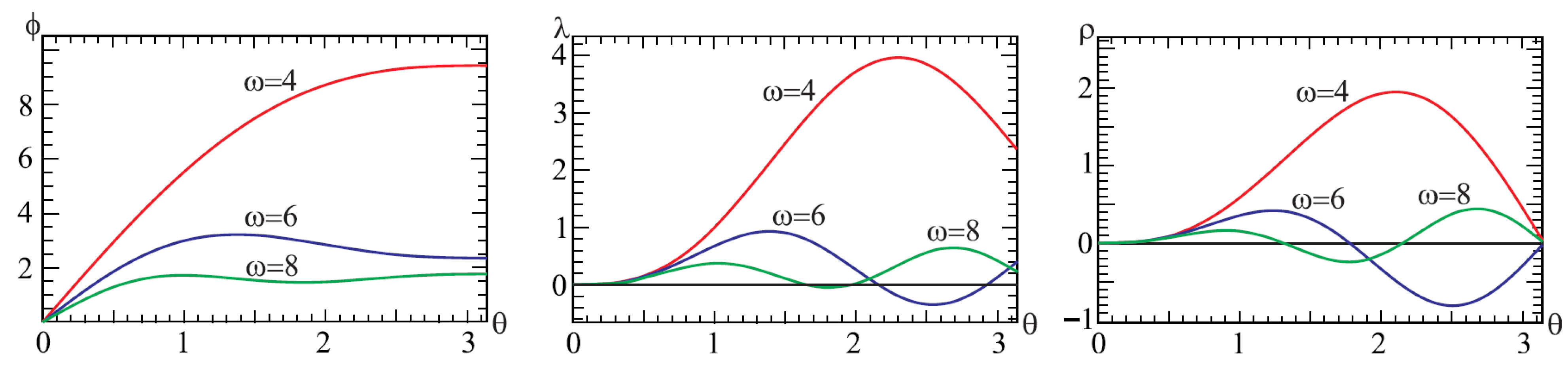
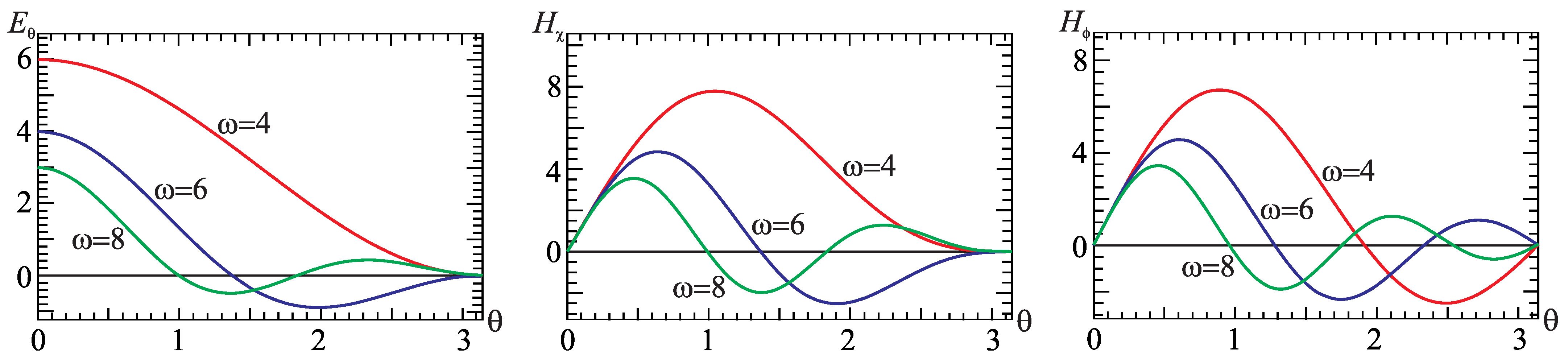
In Section 4.1, the numerical study of solutions within classical electrodynamics has been carried out, and we gave arguments to claim that these solutions form a discrete spectrum. The same situation also takes place for the Dirac equation. The reason for that is that a three-dimensional sphere on the Hopf bundle $S^3\to S^2$ is a compact space; as a result, the spectra of solutions of the Dirac and Maxwell equations are discrete.

For such a case, the operator of the electromagnetic field four-potential can be written in the form

$$\begin{array}{lll}{\widehat{A}}_{\mu }\hfill & =& \sum _{p,q,n}\left[{\widehat{a}}_{pqn}{e}^{i\left(\frac{{\omega }_{pqn}}{r}t+p\chi +q\phi \right)}{\left({\tilde{A}}_{\mu }\right)}_{pqn}\left(\theta \right)+{\left({\widehat{a}}_{pqn}\right)}^{†}{e}^{-i\left(\frac{{\omega }_{pqn}}{r}t+p\chi +q\phi \right)}{\left({\tilde{A}}_{\mu }\right)}_{pqn}\left(\theta \right)\right]\\ & =& {\widehat{A}}_{\mu }^{(+)}+{\widehat{A}}_{\mu }^{(-)}\end{array}$$

(71)

with the following standard commutation relations for the creation, ${\left({\widehat{a}}_{pqn}\right)}^{†}$, and annihilation, ${\widehat{a}}_{pqn}$, operators of the quantum state $\left|pqn\right.〉$:

$$\left[{\widehat{a}}_{pqn},{\left({\widehat{a}}_{rsm}\right)}^{†}\right]=f_{pqn}{\delta }_{pr}{\delta }_{qs}{\delta }_{nm}(\mathrm{all}\mathrm{other}\mathrm{commutators}\mathrm{are}\mathrm{zero}).$$

As for the anticommutation relations (66) and (67), here we have introduced the numerical factor $f_{pqn}$, which will possibly be needed to ensure the finiteness of the sum over the quantum states $pqn$. The momentum operators conjugate to the potential $A_{\mu }$ are defined as

$$\begin{array}{cc}\hfill {\widehat{\pi }}^0& =0,\hfill \\ \hfill {\widehat{\pi }}^{\chi }=-{\widehat{F}}^{0\chi }={\widehat{E}}^{\chi }=& \frac{-4i}{r^2}\sum _{p,q,n}\left[{\widehat{a}}_{pqn}{e}^{i\left(\frac{{\omega }_{pqn}}{r}t+p\chi +q\phi \right)}+{\left({\widehat{a}}_{pqn}\right)}^{†}{e}^{-i\left(\frac{{\omega }_{pqn}}{r}t+p\chi +q\phi \right)}\right]\hfill \\ \hfill \times & \frac{\omega \left({\lambda }_{pqn}cos\theta +{\rho }_{pqn}\right)-{\varphi }_{pqn}\left(p+qcos\theta \right)}{{sin}^2\theta },\hfill \\ \hfill {\widehat{\pi }}^{\theta }=-{\widehat{F}}^{0\theta }={\widehat{E}}^{\theta }=& \frac{4}{r^2}\sum _{p,q,n}\left[{\widehat{a}}_{pqn}{e}^{i\left(\frac{{\omega }_{pqn}}{r}t+p\chi +q\phi \right)}+{\left({\widehat{a}}_{pqn}\right)}^{†}{e}^{-i\left(\frac{{\omega }_{pqn}}{r}t+p\chi +q\phi \right)}\right]{\varphi }^{\prime },\hfill \\ \hfill {\widehat{\pi }}^{\phi }=-{\widehat{F}}^{0\phi }={\widehat{E}}^{\phi }=& \frac{-4i}{r^2}\sum _{p,q,n}\left[{\widehat{a}}_{pqn}{e}^{i\left(\frac{{\omega }_{pqn}}{r}t+p\chi +q\phi \right)}+{\left({\widehat{a}}_{pqn}\right)}^{†}{e}^{-i\left(\frac{{\omega }_{pqn}}{r}t+p\chi +q\phi \right)}\right]\hfill \\ \hfill \times & \frac{\omega \left({\lambda }_{pqn}+{\rho }_{pqn}cos\theta \right)-{\varphi }_{pqn}\left(p+qcos\theta \right)}{{sin}^2\theta }.\hfill \end{array}$$

Let us now calculate the commutators:

$$\begin{array}{cc}\hfill \left[{\widehat{A}}_{\mu }^{(+)}\left(t,\chi ,\theta ,\phi \right),{\widehat{A}}_{\nu }^{(-)}\left(t^{\prime },{\chi }^{\prime },{\theta }^{\prime },{\phi }^{\prime }\right)\right]=& \sum _{p,q,n}{e}^{i\left[\frac{{\omega }_{pqn}}{r}\left(t-t^{\prime }\right)+p\left(\chi -{\chi }^{\prime }\right)+q\left(\phi -{\phi }^{\prime }\right)\right]}\hfill \\ \hfill =& {\left({\tilde{A}}_{\mu }\right)}_{pqn}\left(\theta \right){\left({\tilde{A}}_{\nu }\right)}_{pqn}\left({\theta }^{\prime }\right)\hfill \\ \hfill =& -i{G}_{\mu \nu }^{(+)}\left(t-t^{\prime },\chi -{\chi }^{\prime },\theta ,{\theta }^{\prime },\phi -{\phi }^{\prime }\right),\hfill \\ \hfill \left[{\widehat{A}}_{\mu }^{(-)}\left(t,\chi ,\theta ,\phi \right),{\widehat{A}}_{\nu }^{(+)}\left(t^{\prime },{\chi }^{\prime },{\theta }^{\prime },{\phi }^{\prime }\right)\right]=& -\left[{\widehat{A}}_{\mu }^{(+)}\left(t,\chi ,\theta ,\phi \right),{\widehat{A}}_{\nu }^{(-)}\left(t^{\prime },{\chi }^{\prime },{\theta }^{\prime },{\phi }^{\prime }\right)\right]\hfill \\ \hfill =& -i{G}_{\mu \nu }^{(-)}\left(t-t^{\prime },\chi -{\chi }^{\prime },\theta ,{\theta }^{\prime },\phi -{\phi }^{\prime }\right).\hfill \end{array}$$

Here it must be mentioned that the Green functions $G_{\mu \nu }^{(\pm )}$ are not translationally invariant, since they contain the product ${\left({\tilde{A}}_{\mu }\right)}_{pqn}\left(\theta \right){\left({\tilde{A}}_{\nu }\right)}_{pqn}\left({\theta }^{\prime }\right)$. These expressions permit us to calculate the Feynman Green’s function

$$\begin{array}{cc}\hfill G_{F,\mu \nu }=& -{\Theta }\left(t-t^{\prime }\right)G_{\mu \nu }^{(+)}\left(t-t^{\prime },\chi -{\chi }^{\prime },\theta ,{\theta }^{\prime },\phi -{\phi }^{\prime }\right)\hfill \\ \hfill & +{\Theta }\left(t^{\prime }-t\right)G_{\mu \nu }^{(-)}\left(t-t^{\prime },\chi -{\chi }^{\prime },\theta ,{\theta }^{\prime },\phi -{\phi }^{\prime }\right).\hfill \end{array}$$

(72)

The results that were obtained in this section concerning the quantization of free Dirac and Maxwell fields need to be compared with the usual quantization in a box in Minkowski spacetime. The main difference is that, in the box eigenfunctions, are plain waves (because the spacetime is locally flat). On a sphere, plain waves cannot be eigenfunctions of the Dirac equation, since the spacetime has a nonzero curvature. For this reason, the propagators are not translationally invariant; they are functions of $\theta ,{\theta }^{\prime }$, but not functions of their difference, $(\theta -{\theta }^{\prime })$.

6. Nonperturbative Quantization of Maxwell’s Electrodynamics Coupled to a Spinor Field

In this section, we suggest a method of nonperturbative quantization of Maxwell–Dirac theory on the Hopf bundle. As we saw in Section 5, a fact of compactness of a three-dimensional sphere $S^3$ very much simplifies the procedure of the quantization of free fields: when quantizing, no Dirac delta functions appear, since they are replaced by the Kronecker symbols. This would lead us to expect that the quantization of interacting fields on a sphere $S^3$ will also be considerably simplified. Additionally, notice that there appears to be a considerable difference in the behavior of quantum fields on a sphere $S^3$ and in Minkowski space: the propagators of free fields on the compact space are not translationally invariant.

According to Heisenberg [5], the process of nonperturbative quantization consists in that a set of equations describing interacting fields [ in our case, these are Equations (2) and (3)] written in the operator form

$$\begin{array}{cc}\hfill i{\gamma }^{\mu }{\widehat{\psi }}_{;\mu }=& 0,\hfill \end{array}$$

(73)

$$\begin{array}{cc}\hfill \frac{1}{\sqrt{-g}}\frac{\partial }{\partial x^{\nu }}\left(\sqrt{-g}{\widehat{F}}^{\mu \nu }\right)=& -4\pi {\widehat{j}}^{\mu },\hfill \end{array}$$

(74)

where the covariant derivative of the spinor field, the operators of the field strength and of the current are defined as ${\widehat{\psi }}_{;\mu }=\left[{\partial }_{\mu }+1/8{\omega }_{ab\mu }\left({\gamma }^a{\gamma }^b-{\gamma }^b{\gamma }^a\right)-ie{\widehat{A}}_{\mu }\right]\widehat{\psi },{\widehat{F}}_{\mu \nu }={\partial }_{\mu }{\widehat{A}}_{\nu }-{\partial }_{\nu }{\widehat{A}}_{\mu }$, and ${\widehat{j}}^{\mu }=e\widehat{\overline{\psi }}{\gamma }^{\mu }\widehat{\psi }$, respectively.

It is worth pointing out that the above equations involve the operators of the interacting fields $\widehat{\psi }$ and ${\widehat{A}}_{\mu }$, whose properties differ from those of free, noninteracting fields considered in the previous section. Notice also the presence of the nonlinear quantities ${\widehat{A}}_{\mu }\widehat{\psi }$ and $\widehat{\overline{\psi }}{\gamma }^{\mu }\widehat{\psi }$. The former describes the interaction between the fields, and the latter is the source of the electromagnetic field. These nonlinear quantities do not allow for quantizing the fields $\psi$ and $A_{\mu }$, as was done in Section 5. For free fields, we have discrete spectra of solutions, a linear combination of which permits one to find any solution to the Maxwell or Dirac equations. With such spectra in hand, one can quantize the fields by writing the operators $\widehat{\psi }$ and ${\widehat{A}}_{\mu }$ as a superposition of solutions of the discrete spectrum and by introducing the creation and annihilation operators of the corresponding quantum states, which are the coefficients before each such solution. In Minkowski space, such operators are called the creation/annihilation operators for particles. However, in our case, we cannot speak of particles, since the functions (32) and (43) do not correspond to plane waves.

When quantizing free fields, we saw that the propagators (69) and (72) are ordinary (not distribution) functions. These propagators do not involve Dirac delta functions and, therefore, the product of two operators at one point is well defined. This was demonstrated for the propagator $S_{\alpha \beta }(0,0,\theta ,\theta ,0)$ in Section 5.1. It is reasonable to expect that this property also persists for the operators of interacting fields. Hence, the products of the interacting operators ${\widehat{A}}_{\mu }\widehat{\psi }$ and $\widehat{\overline{\psi }}{\gamma }^{\mu }\widehat{\psi }$ for the discrete spectrum on the Hopf bundle are well defined, in contrast to the same product of operators of free fields in the case of perturbative quantization in Minkowski space.

According to Reference [5], the main idea of nonperturbative quantization consists in that the operator Equations (73) and (74) are replaced by an infinite system for all Green’s functions. The first equations are the quantum average of Equations (73) and (74). They contain the Green functions $G(A_{\mu }\left(x\right),\psi \left(y\right))=〈{\widehat{A}}_{\mu }\left(x\right)\widehat{\psi }\left(y\right)〉$ and $G(\overline{\psi }\left(x\right),\psi \left(y\right))=〈\widehat{\overline{\psi }}\left(x\right)\widehat{\psi }\left(y\right)〉$. It is necessary to derive equations for these Green functions in order to close the set of equations. To do this, the operator Equations (73) and (74) are multiplied by the corresponding operators and they are averaged; this is done an infinite number of times. As a result, one arrives at the following infinite set of equations:

$$\begin{array}{cc}\hfill i{\gamma }^{\mu }〈{\widehat{\psi }}_{;\mu }〉=& 0,\hfill \end{array}$$

(75)

$$\begin{array}{cc}\hfill \frac{1}{\sqrt{-g}}\frac{\partial }{\partial x^{\nu }}\left(\sqrt{-g}〈{\widehat{F}}^{\mu \nu }〉\right)=& -4\pi 〈{\widehat{j}}^{\mu }〉,\hfill \end{array}$$

(76)

$$\begin{array}{cc}\hfill i{\gamma }^{\mu }〈\widehat{\overline{\psi }}{\widehat{\psi }}_{;\mu }〉=& 0,\hfill \end{array}$$

(77)

$$\begin{array}{cc}\hfill i{\gamma }^{\mu }〈{\widehat{A}}_{\nu }{\widehat{\psi }}_{;\mu }〉=& 0,\hfill \end{array}$$

(78)

$$\begin{array}{cc}\hfill \frac{1}{\sqrt{-g}}\frac{\partial }{\partial x^{\nu }}\left(\sqrt{-g}〈{\widehat{F}}^{\mu \nu }\widehat{\psi }〉\right)=& -4\pi 〈{\widehat{j}}^{\mu }\widehat{\psi }〉,\hfill \end{array}$$

(79)

$$\begin{array}{c}\hfill \dots \end{array}$$

(80)

Note that the Green function $G(A_{\mu }\left(x\right),\psi \left(y\right))$ is a function of two variables and, for its definition, we need two Equations (78) and (79). After adding the Equations (77)–(79), there appear new Green’s functions $〈\widehat{\overline{\psi }}{\widehat{A}}_{\mu }\widehat{\psi }〉$, $〈{\widehat{A}}_{\nu }{\widehat{A}}_{\mu }\widehat{\psi }〉$, and $〈\widehat{\overline{\psi }}\widehat{\psi }\widehat{\psi }〉$, for which one has to write out new equations, and so on an infinite number of times [this is denoted by Equation (80)].

It is evident that this infinite set of equations cannot be explicitly and analytically solved. Therefore, the question arises as to whether it is possible to find its approximate solution. The problem of how to cut off an infinite set of equations is called the closure problem, and it is well known in turbulence modeling (see, e.g., the textbook [11]). In that case, the Navier–Stokes equation is averaged, and it is known as the Reynolds-averaged Navier–Stokes equation. However, this equation contains an unknown quantity—the Reynolds-stress tensor, for which one has to have an extra equation, called the Reynolds-stress equation, which, in turn, contains more unknown functions, and so on.

For a better understanding of the situation, it is useful to consider some simple example illustrating this process. Consider the case where, to solve the set of Equations (75)–(80), one can employ the simplified $\mathfrak{Ansatze}$ (5) for the spinor field and (6) for the potential of the electromagnetic field:

$${{\Theta }}_2=\pm {{\Theta }}_1=\pm {\Theta },{\tilde{{\Omega }}}_{n0}=\frac{1}{4}-\frac{r{\Omega }}{2}=\pm n,\varphi =\mp 2\rho .$$

(81)

This case is a special case of the general $\mathfrak{Ansatze}$ (5), and it corresponds to the particular solution for $l=0$ found in Reference [12].

Replacing the functions by operators, we then have

$${\widehat{\psi }}_{nm0}=e^{-i{\Omega }t}{e}^{in\chi }{e}^{im\phi }{\widehat{{\Theta }}}_{nm0}\left(\theta \right)\left(\begin{array}{c}1\\ \pm 1\\ 0\\ 0\end{array}\right),{\widehat{A}}_{\mu }=\left\{\widehat{\varphi }\left(\theta \right),r\widehat{\rho }\left(\theta \right),0,r\widehat{\lambda }\left(\theta \right)\right\}.$$

(In what follows, we drop the indices $n,m,0$ by $\widehat{{\Theta }}$ for brevity.) In this case we obtain the following equations coming from the quantum Equations (75)–(80):

$$\begin{array}{cc}\hfill {\widehat{{\Theta }}}^{\prime }\mp \widehat{{\Theta }}\left[cot\theta \left(\mp \frac{1}{2}+n+er\widehat{\rho }\right)+\frac{1}{sin\theta }\left(m+er\widehat{\lambda }\right)\right]& =0,\hfill \end{array}$$

(82)

$$\begin{array}{cc}\hfill \frac{1}{sin\theta }{\left(sin\theta {\widehat{\varphi }}^{\prime }\right)}^{\prime }& =-e{r}^{3/2}\frac{{\widehat{{\Theta }}}^2}{2},\hfill \end{array}$$

(83)

$$\begin{array}{cc}\hfill \frac{1}{sin\theta }{\left(sin\theta {\widehat{\rho }}^{\prime }\right)}^{\prime }& =\pm e{r}^{3/2}\frac{{\widehat{{\Theta }}}^2}{4},\hfill \end{array}$$

(84)

$$\begin{array}{cc}\hfill {\widehat{\lambda }}^{\prime }& =-{\widehat{\rho }}^{\prime }cos\theta .\hfill \end{array}$$

(85)

After quantum averaging, the first Equation (82) will be the equation for $〈\widehat{{\Theta }}〉$, the second one—for $〈\widehat{\varphi }〉$, the third one— for $〈\widehat{\rho }〉$, and the fourth one— for $〈\widehat{\lambda }〉$. However, these equations contain the following new Green’s functions:

$$G_{{\Theta }\rho }({\theta }_1,{\theta }_2)=〈\widehat{{\Theta }}\left({\theta }_1\right)\widehat{\rho }\left({\theta }_2\right)〉,G_{{\Theta }\lambda }({\theta }_1,{\theta }_2)=〈\widehat{{\Theta }}\left({\theta }_1\right)\widehat{\lambda }\left({\theta }_2\right)〉,G_{{\Theta }{\Theta }}({\theta }_1,{\theta }_2)=〈\widehat{{\Theta }}\left({\theta }_1\right)\widehat{{\Theta }}\left({\theta }_2\right)〉,$$

for which one must have their own equations. The equation for the Green function $G_{{\Theta }\rho }(x,y)$ can be obtained by multiplying the operator Equation (82) on the right by $\widehat{\rho }$ and by performing the quantum averaging,

$$G_{\overline{{\Theta }}\rho }^{\prime }\mp G_{{\Theta }\rho }\left[cot\theta \left(\mp \frac{1}{2}+n\right)+\frac{m}{sin\theta }\right]\mp er〈\widehat{{\Theta }}{\widehat{\rho }}^2〉\mp er〈\widehat{{\Theta }}\widehat{\lambda }\widehat{\rho }〉=0,$$

where we have introduced the following notation:

$$G_{\overline{{\Theta }}\rho }^{\prime }(\theta ,\theta )={\left.\frac{d{G}_{{\Theta }\left(\theta \right)\rho \left({\theta }^{\prime }\right)}}{d\theta }\right|}_{{\theta }^{\prime }=\theta }.$$

Here, $\overline{{\Theta }}$ denotes that the derivative is taken with respect to the function ${\Theta }$ with the bar. The Green function $G_{{\Theta }\rho }({\theta }_1,{\theta }_2)$ is a function of two variables ${\theta }_1$ and ${\theta }_2$; hence, one has to have one more differential equation for the variable ${\theta }_2$. This equation can be obtained by multiplying the Equation (84) on the left by $\widehat{{\Theta }}$, and by performing the quantum averaging,

$$\frac{1}{sin\theta }{\left(sin\theta G_{{\Theta }\overline{\rho }}^{\prime }\right)}^{\prime }=\pm e{r}^{3/2}\frac{〈{\widehat{{\Theta }}}^3〉}{4}.$$

Similarly, one can obtain equations for the Green functions $G_{{\Theta }\lambda }({\theta }_1,{\theta }_2)$ and $G_{{\Theta }{\Theta }}({\theta }_1,{\theta }_2)$. As a result, we arrive at an infinite set of equations for an infinite number of Green’s functions

$$\begin{array}{cc}\hfill {〈\widehat{{\Theta }}〉}^{\prime }\mp 〈\widehat{{\Theta }}〉\left[cot\theta \left(\mp \frac{1}{2}+n\right)+\frac{m}{sin\theta }\right]\mp er{G}_{{\Theta }\rho }\mp er{G}_{{\Theta }\lambda }& =0,\hfill \end{array}$$

(86)

$$\begin{array}{cc}\hfill \frac{1}{sin\theta }{\left(sin\theta {〈\widehat{\varphi }〉}^{\prime }\right)}^{\prime }& =-e{r}^{3/2}\frac{G_{{\Theta }{\Theta }}}{2},\hfill \end{array}$$

(87)

$$\begin{array}{cc}\hfill \frac{1}{sin\theta }{\left(sin\theta {〈\widehat{\rho }〉}^{\prime }\right)}^{\prime }& =\pm e{r}^{3/2}\frac{G_{{\Theta }{\Theta }}}{4},\hfill \end{array}$$

(88)

$$\begin{array}{cc}\hfill {〈\widehat{\lambda }〉}^{\prime }& =-{〈\widehat{\rho }〉}^{\prime }cos\theta ,\hfill \end{array}$$

(89)

$$\begin{array}{cc}\hfill G_{\overline{{\Theta }}\rho }^{\prime }\mp G_{{\Theta }\rho }\left[cot\theta \left(\mp \frac{1}{2}+n\right)+\frac{m}{sin\theta }\right]\mp er〈\widehat{{\Theta }}{\widehat{\rho }}^2〉\mp er〈\widehat{{\Theta }}\widehat{\lambda }\widehat{\rho }〉& =0,\hfill \end{array}$$

(90)

$$\begin{array}{cc}\hfill \frac{1}{sin\theta }{\left(sin\theta G_{{\Theta }\overline{\rho }}^{\prime }\right)}^{\prime }& =\pm e{r}^{3/2}\frac{〈{\widehat{{\Theta }}}^3〉}{4},\hfill \end{array}$$

(91)

$$\begin{array}{cc}\hfill G_{\overline{{\Theta }}\lambda }^{\prime }\mp G_{{\Theta }\lambda }\left[cot\theta \left(\mp \frac{1}{2}+n\right)+\frac{m}{sin\theta }\right]\mp er〈\widehat{{\Theta }}\widehat{\rho }\widehat{\lambda }〉\mp er〈\widehat{{\Theta }}{\widehat{\lambda }}^2〉& =0,\hfill \end{array}$$

(92)

$$\begin{array}{cc}\hfill G_{{\Theta }\overline{\lambda }}^{\prime }& =-G_{{\Theta }\overline{\rho }}^{\prime }cos\theta ,\hfill \end{array}$$

(93)

$$\begin{array}{cc}\hfill G_{\overline{{\Theta }}{\Theta }}^{\prime }\mp G_{{\Theta }{\Theta }}\left[cot\theta \left(\mp \frac{1}{2}+n\right)+\frac{m}{sin\theta }\right]\mp er〈\widehat{{\Theta }}\widehat{\rho }\widehat{{\Theta }}〉\mp er〈\widehat{{\Theta }}\widehat{\lambda }\widehat{{\Theta }}〉& =0.\hfill \end{array}$$

(94)

$$\begin{array}{cc}\hfill \cdots & =\cdots \hfill \end{array}$$

(95)

As expected, Equations (90), (92), and (94) contain new three-point Green’s functions,

$$\begin{array}{c}\hfill \begin{array}{cc}\hfill G_{{\Theta }\rho \rho }\left({\theta }_1,{\theta }_2,{\theta }_3\right)& =〈\widehat{{\Theta }}\left({\theta }_1\right)\widehat{\rho }\left({\theta }_2\right)\widehat{\rho }\left({\theta }_3\right)〉,G_{{\Theta }\lambda \rho }\left({\theta }_1,{\theta }_2,{\theta }_3\right)=〈\widehat{{\Theta }}\left({\theta }_1\right)\widehat{\lambda }\left({\theta }_2\right)\widehat{\lambda }\left({\theta }_3\right)〉,\hfill \\ \hfill G_{{\Theta }{\Theta }{\Theta }}\left({\theta }_1,{\theta }_2,{\theta }_3\right)& =〈\widehat{{\Theta }}\left({\theta }_1\right)\widehat{{\Theta }}\left({\theta }_2\right)\widehat{{\Theta }}\left({\theta }_3\right)〉,G_{{\Theta }\rho \lambda }\left({\theta }_1,{\theta }_2,{\theta }_3\right)=〈\widehat{{\Theta }}\left({\theta }_1\right)\widehat{\rho }\left({\theta }_2\right)\widehat{\lambda }\left({\theta }_3\right)〉,\hfill \\ \hfill G_{{\Theta }\lambda \lambda }\left({\theta }_1,{\theta }_2,{\theta }_3\right)& =〈\widehat{{\Theta }}\left({\theta }_1\right)\widehat{\lambda }\left({\theta }_2\right)\widehat{\lambda }\left({\theta }_3\right)〉,G_{{\Theta }\rho {\Theta }}\left({\theta }_1,{\theta }_2,{\theta }_3\right)=〈\widehat{{\Theta }}\left({\theta }_1\right)\widehat{\rho }\left({\theta }_2\right)\widehat{{\Theta }}\left({\theta }_3\right)〉,\hfill \\ \hfill G_{{\Theta }\lambda {\Theta }}\left({\theta }_1,{\theta }_2,{\theta }_3\right)& =〈\widehat{{\Theta }}\left({\theta }_1\right)\widehat{\lambda }\left({\theta }_2\right)\widehat{{\Theta }}\left({\theta }_3\right)〉,\hfill \end{array}\end{array}$$

for which, in turn, one has to have differential equations that determine these Green’s functions. As a result of this process, we finally obtain an infinite set of differential equations describing all of Green’s functions of the operators $\widehat{{\Theta }},\widehat{\rho },\widehat{\varphi },$ and $\widehat{\lambda }$ appearing in the operator Equations (82)–(85).

As was mentioned above, the infinite set of equations obtained can scarcely be solved explicitly and, hence, the question of its approximate solving arises. Using the experience accumulated in turbulence modeling, one can assume that this can be done by cutting off the infinite set of equations to a finite one using some physical assumptions concerning higher-order Green’s functions. In doing so, one can involve the following suppositions:

• one can neglect $n-$th order Green’s functions compared with $(n-1)-$th order Green’s functions;
• $n-$th order Green’s functions are polylinear combinations of lower-order Green’s functions;
• one can use the energy conservation law together with some physically reasonable propositions concerning its separate components; and,
• so on…

7. Discussion and Conclusions

We have considered the Dirac equation and Maxwell’s electrodynamics in $\mathbb{R}\times S^3$ spacetime. The distinctive feature of these theories on the Hopf bundle is that they have discrete spectra of solutions both for the Dirac equation and for Maxwell’s electrodynamics. This is a consequence of the fact that a three-dimensional sphere $S^3$ is a compact space. For the Dirac equation, this was explicitly shown by finding discrete solutions in analytic form. For the Maxwell equations, we have obtained numerical solutions, as well as solutions for some particular cases, and the analysis of these solutions permits us to assume that a discrete spectrum of the solutions does exist.

The presence of the discrete spectrum allows for one to quantize the free, noninteracting Dirac and Maxwell fields on the Hopf bundle. For the Dirac equation, the quantization is suggested by introducing the creation and annihilation operators for the corresponding quantum states. The standard anticommutation relations are imposed on these operators, and an additional numerical factor in the right-hand side of the anticommutator is introduced. The propagator for the spinor field is calculated using these relations. The calculations indicate that this propagator is a sum over the discrete spectrum numbered by the quantum numbers $m,n$ and l. It is necessary that the aforementioned factor would possess a perfectly definite dependence on the quantum number $n,m,l$ in order to ensure the convergence of the sum.

For the free electromagnetic field, a similar scheme of quantization has been suggested.

The most important part of the present study is the procedure of nonperturbative quantization suggested for the interacting Dirac and Maxwell fields. Following Heisenberg [5], we have replaced the classical equations by equations for operators of the corresponding fields. Because the operator equation can scarcely be solved somehow, it is replaced by an infinite set of equations for Green’s functions. Such a set is known as the Schwinger–Dyson equations, but they are usually employed in perturbative quantum field theory.

We have considered some physical system possessing perfectly definite $\mathfrak{Ansatze}$ for the spinor and electromagnetic fields in order to illustrate the suggested scheme of nonperturbative quantization. This gives the much more simple set of equations, for which we have written out the first few equations for one- and two-point Green’s functions. For the equations describing two-point Green’s functions, we have explicitly written out three-point Green’s functions appearing in these equations.

The significance of examination of the scheme of nonperturbative quantization is that if, in nature, some fields are quantized, then apparently there should exist a mathematically well-defined quantization procedure for any field, including those that are not quantized due to the perturbative nonrenormalizibilty of the theory.

Let us note some features of the nonperturbative quantization.

• The properties of the operators of interacting fields can differ drastically from those of free fields. For example, in the quantum theory of strongly interacting fields, there can exist static field configurations that are similar to those that were described by soliton, monopole, instanton, etc. solutions in classical field theory.
• The properties of the operators of interacting fields cannot be assigned by their commutators/anticommutators. The algebra of these fields is much more complicated when compared with the algebra given only by commutators/anticommutators. These properties are determined by the infinite set of the Schwinger–Dyson equations as a whole.
• For strongly interacting quantum fields, it is impossible to introduce creation and annihilation operators, since the field operators cannot be represented as a superposition of plane waves with the coefficients that are creation and annihilation operators.
• Separate consideration of the notion of quantum state is required, since, in perturbative quantum field theory, quantum states are defined using creation and annihilation operators. According to what has been said in the previous item, such operators cannot be defined for strongly interacting fields, and, hence, the definition of quantum states requires special consideration.
• It is possible that the properties of the operators of interacting fields and of quantum states are related to the properties of the complete set of Green’s functions that are defined by the Schwinger–Dyson equations.

References

1. Landau, L.D.; Abrikosov, A.A.; Khalatnikov, I.M. The removal of infinities in quantum electrodynamics. Dokl. Akad. Nauk SSSR 1954, 95, 497–500. (In Russian) [Google Scholar]
2. Landau, L.D.; Abrikosov, A.A.; Khalatnikov, I.M. An asymptotic expression for the electron Green function in quantum electrodynamics. Dokl. Akad. Nauk SSSR 1954, 95, 773–776. (In Russian) [Google Scholar]
3. Landau, L.D.; Abrikosov, A.A.; Khalatnikov, I.M. An asymptotic expression for the photon Green function in quantum electrodynamics. Dokl. Akad. Nauk SSSR 1954, 95, 1177–1180. (In Russian) [Google Scholar]
4. Landau, L.D.; Abrikosov, A.A.; Khalatnikov, I.M. The electron mass in quantum electrodynamics. Dokl. Akad. Nauk SSSR 1954, 96, 261–265. (In Russian) [Google Scholar]
5. Heisenberg, W. Introduction to the Unified Field Theory of Elementary Particles; Interscience Publishers: London, UK, 1966; p. 239. [Google Scholar]
6. Dzhunushaliev, V.; Folomeev, V. Dirac/Rarita-Schwinger plus Maxwell theories in R × S 3 spacetime in the Hopf coordinates. Int. J. Geom. Meth. Mod. Phys. 2020, 17, 2050197. [Google Scholar] [CrossRef]
7. Lawrie, I. A Unified Grand Tour of Theoretical Physics; Institute of Physics Publishing: Bristol, UK, 2002. [Google Scholar]
8. Carmeli, M.; Malin, S. Field Theory on R × S3 Topology. 3. The Dirac Equation. Found. Phys. 1985, 15, 1019–1029. [Google Scholar] [CrossRef]
9. Alves, D.W.F.; Hoyos, C.; Nastase, H.; Sonnenschein, J. Knotted solutions for linear and nonlinear theories: Electromagnetism and fluid dynamics. Phys. Lett. B 2017, 773, 412–416. [Google Scholar] [CrossRef]
10. Busse, K. Eigenlösungen der Maxwellgleichung auf S1 × S3 und Konforme Symmetrie, Untersuchungen am U(2)-Programm. Ph.D. Thesis, Martin Luther University of Halle-Wittenberg, Halle, Germany. Available online: http://sundoc.bibliothek.uni-halle.de/diss-online/98/98H152/prom.pdf (accessed on 30 January 2021).
11. Wilcox, D.C. Turbulence Modeling for CFD; DCW Industries, Inc.: Acheson, AB, Canada, 1994; p. 217. [Google Scholar]
12. Dzhunushaliev, V.; Folomeev, V. Spinor field solutions in F(B2) modified Weyl gravity. Int. J. Mod. Phys. D 2020, 29, 2050094. [Google Scholar] [CrossRef]
Figure 1. The profiles of A t = ϕ ( θ ) , A φ = λ ( θ ) , and A χ = ρ ( θ ) for λ 0 = ρ 0 = 1 .
Universe 07 00065 g001
Figure 2. The profiles of the electric field E θ = ϕ ( θ ) and magnetic fields H χ = 2 λ + cos θ ρ sin θ and H φ = 2 ρ + cos θ λ sin θ . For all graphs λ 0 = ρ 0 = 1 .
Universe 07 00065 g002
Publisher’s Note: MDPI stays neutral with regard to jurisdictional claims in published maps and institutional affiliations.