Communication

Precision Measurement Noise Asymmetry and Its Annual Modulation as a Dark Matter Signature

by
Benjamin M. Roberts
1,2 and
Andrei Derevianko
2,*
1
School of Mathematics and Physics, The University of Queensland, Brisbane, QLD 4072, Australia
2
Department of Physics, University of Nevada, Reno, NV 89557, USA
*
Author to whom correspondence should be addressed.
Universe 2021, 7(3), 50; https://doi.org/10.3390/universe7030050
Submission received: 21 January 2021 / Revised: 15 February 2021 / Accepted: 24 February 2021 / Published: 28 February 2021
(This article belongs to the Special Issue Advances in Understanding Astrophysical and Atomic Phenomena)

Abstract

:
Dark matter may be composed of self-interacting ultralight quantum fields that form macroscopic objects. An example of which includes Q-balls, compact non-topological solitons predicted by a range of theories that are viable dark matter candidates. As the Earth moves through the galaxy, interactions with such objects may leave transient perturbations in terrestrial experiments. Here we propose a new dark matter signature: an asymmetry (and other non-Gaussianities) that may thereby be induced in the noise distributions of precision quantum sensors, such as atomic clocks, magnetometers, and interferometers. Further, we demonstrate that there would be a sizeable annual modulation in these signatures due to the annual variation of the Earth velocity with respect to dark matter halo. As an illustration of our formalism, we apply our method to 6 years of data from the atomic clocks on board GPS satellites and place constraints on couplings for macroscopic dark matter objects with radii R < 10 4 km , the region that is otherwise inaccessible using relatively sparse global networks.

1. Introduction

Multiple astrophysical observations suggest that the ordinary (luminous or baryonic) matter contributes only ∼5% to the total energy density budget of the universe. Exacting the microscopic nature of the two other constituents, dark matter (DM) and dark energy remains a grand challenge to modern physics and cosmology. DM is required for galaxy formations, while dark energy leads to the accelerated expansion of the universe. The distinction between DM and dark energy can be formalized by treating them as cosmological fluids: they have different equations of state, DM is being pressureless, while dark energy exerts negative pressure. For further details the reader is referred to the cosmology textbooks, e.g., Ref. [1] and reviews such as [2,3,4,5].
Exacting the microscopic nature of DM and its non-gravitational interaction with the standard model particles and fields is challenging. Indeed, all the evidence for DM (galactic rotation curves, gravitational lensing, peaks in the cosmic microwave background spectra, etc) comes from galactic scale (parsecs) observations. The challenge lies in extrapolating down from these scales to the laboratory scales and a large number of theoretical models can fit the observations. All the theoretical constructs are guided by the cold dark matter paradigm that describes the large-scale structure formation of the universe [6].
Despite composing the majority of matter in the universe, the microscopic nature of DM remains a mystery. Most of the particle physics experiments so far have focused on weakly-interacting massive particles (WIMPs) with ∼GeV – TeV masses. Despite the extensive effort, there is no solid evidence for WIMPs in such ambitious large-scale experiments [7,8,9]. Besides WIMPs, there are a multitude of other DM candidates with masses that span many orders of magnitude. Even if DM constituents are elementary particles, their masses can plausibly span 50 orders of magnitude: from 10 22 eV to 10 28 eV , with the lower bound coming from the requirements that their de Broglie wavelengths fit into dwarf galaxies, and the upper bound coming from the condition that they do not form black holes.
Considering a wide variety of DM models, here we focus on ultralight ( m ϕ < 10 eV ) scalar field candidates characterized by high mode occupation numbers (≫1); these can be described as classical fields. The question of microstructure of DM is an open question [10]. We simply split such fields into dichotomy of being either non-self-interacting or self-interacting. In the former case they are nearly uniformly distributed over the galaxies providing a uniform DM field background primarily oscillating at their Compton frequencies (“wavy” DM). Such candidates include pseudo-scalar axions and scalar dilatons/moduli. In the case of self-interacting DM fields, of interest to our paper, self-interactions can lead to formation of clumps. Then DM can be viewed as a gas-like collection of gravitationally interacting clumps. Encounters with such objects may leave transient signals in measurement device data [11,12]. Examples of “clumpy” DM models include Q-balls [13,14,15,16], Bose stars [17,18,19], topological defects [20,21,22], axion quark nuggets [23,24,25] and “dark blobs” [26].
A formation of DM clumps in the radiation era has been analyzed recently in Ref. [27]. The clump formation requires non-linear self-interactions of the scalar DM field. Non-linearities lead to cosmological fluid instability and the fluctuations of the scalar energy-density field lead to the formations of the clumps. Further, the clumps aggregate and afterwards follow the standard cold dark matter scenario. In this model, the gravitationally interacting clumps behave as the pre-requisite pressureless cosmological fluid. The scalar-field mass m ϕ can span a wide range from 10 17 eV to 10 GeV . The formed clumps span a wide range of scales and masses M, ranging from the size of atoms (∼angstroms) to that of galactic molecular clouds (∼parsec), and from a milligram to thousands of solar masses. For the considered range of parameters, the clumps do no collapse into black holes. The clump mass-radius relation follows a power law, M R n , where the power n = 3 , 4 , 5 depends on the details of the formation mechanisms and the self-interaction potential. Because of finite-size effects, these dark matter clumps are shown [27] to evade the microlensing constraints [28].
As we are interested in direct DM detection with laboratory instruments, local properties of DM are essential to interpreting such experiments. At the most basic level, our galaxy, the Milky Way, is embedded into a DM halo and rotates through the halo. Astrophysical simulations provide estimates of DM properties in the Solar system (see, e.g., [29]). The DM energy density in the vicinity of Solar system is estimated to be ρ DM 0.3 GeV / cm 3 , corresponding to ∼one hydrogen atoms per three cm 3 . Further, in the DM halo reference frame, the velocity distribution of DM objects is nearly Maxwellian with the dispersion of v vir 270 km / s (referred to as the virial velocity in the literature) and a sharp cut-off at the galactic escape velocity v esc 650 km / s . Further, the Milky Way is a spiral galaxy rotating through the DM halo. In particular, the Sun moves through the DM halo at galactic velocities v g 230 km / s . For terrestrial experiments, there is an additional velocity modulation arising due to the Earth’s orbital motion about the Sun, modulating the rate of encounters with DM objects. The period, phase, and amplitude of the modulation serve as unique DM signatures [30].
A general challenge with searching for transient signals is that they are difficult to distinguish from conventional noise. One approach [11,31] is to use a network of devices, and search for the correlated propagation of transients that sweep through the network at galactic velocities, v g 300 km / s (see also [24,32,33,34,35,36]). However, objects of spatial extent smaller than the network node separation would not produce such a signature. Then one has to rely on unique signatures of the interactions with a single sensor that may differentiate them from the conventional noise. Gravitational wave searches, for example, use both a correlated signal propagation across a network and a distinct signal pattern at each node [37].
If DM interacts with standard model particles, recurring encounters may cause perturbations in precision sensors. If this were to lead only to a shift in the mean of the data it would be unobservable, as DM is always present. Such interactions may, however, induce non-Gaussian signatures, such as an asymmetry in the data noise distribution, which are observable. Further, we show that there would be an appreciable annual modulation in these signatures, that arises due to the Earth’s orbital motion about the Sun, modulating the rate of encounters with DM objects.
Following these ideas, one may perform DM searches that are many orders of magnitude more sensitive than the existing constraints for certain models, and have discovery reach inaccessible by other means. Our proposal is complimentary to other ultralight DM searches, e.g., [36,38,39,40,41,42,43,44,45,46]. The technique proves particularly appealing for the parameter space of small clumps or high number density objects, where the expected encounter rate may be high. Moreover, such searches may be performed using existing quantum sensors, making this an inexpensive avenue for potential discovery. Finally, we note that while we focus on atomic clocks, the presented ideas apply also to other precision instruments, such as magnetometers [16,31], interferometers [47,48,49], gravimeters [50,51], optical cavities [45,52], and dipole moment searches [53,54,55,56].

2. Results

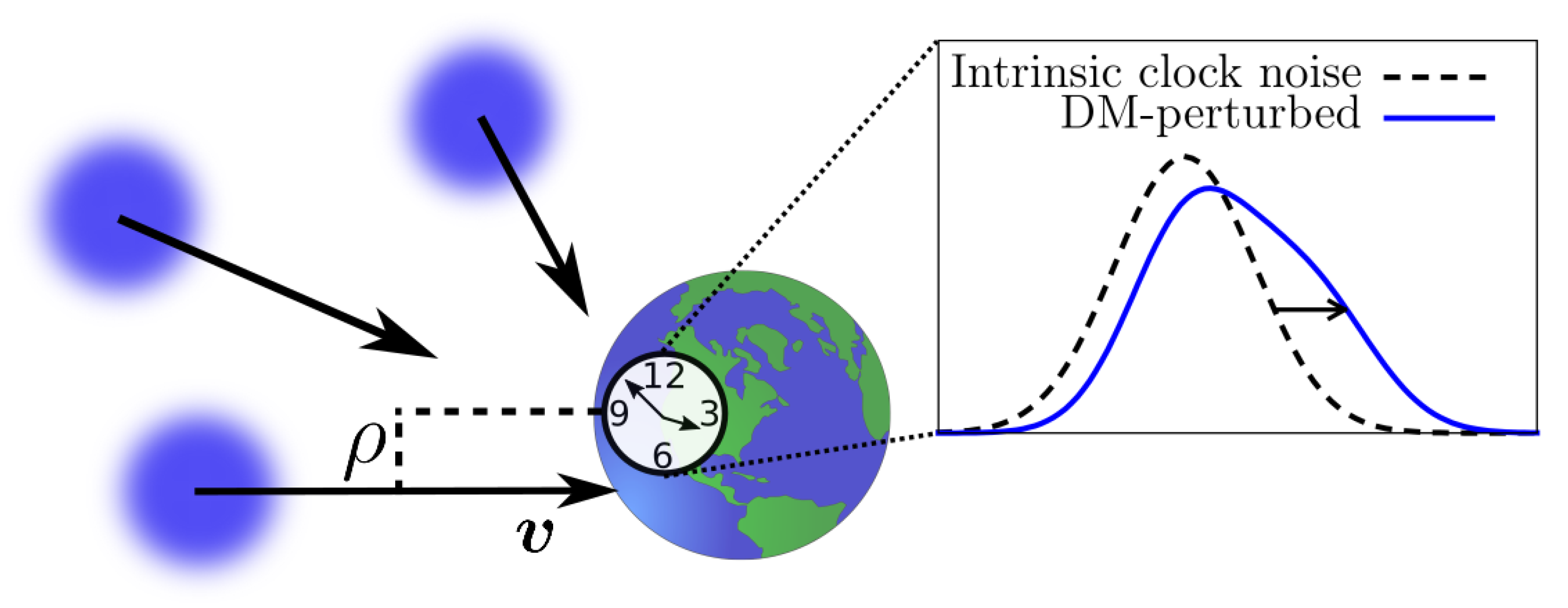
2.1. Dark Matter and Atomic Clocks

We consider interactions that lead to transient shifts in atomic transition frequencies of the form:
δ ν / ν c | ϕ ( r , t ) | 2 ,
where ν c is the unperturbed frequency, and ϕ is the DM field. The proportionality constant depends on the DM model and the sensor. As shown below, such interactions with macroscopic DM objects lead to an asymmetry in the noise distribution, as depicted in Figure 1.
The frequency excursion (1) leads to an additive term, χ , in the time (phase) as measured by the clock:
χ ( t j ) = t j τ 0 t j δ ν ( r , t ) ν c d t ,
where the phase differences (from one data sample to the next) are recorded for discrete values of elapsed time t j . Any DM encounter during the sampling interval will induce a shift in the measured phase.
Now we remark on some generic properties of macroscopic DM objects. We denote the radius of the objects as R, and the energy density inside each object as ρ ϕ . By assuming the objects make up some fraction of total galactic DM density, these can be linked to T , the mean time between consecutive encounters of a given point-like instrument with a DM object as:
T = 4 ρ ϕ R 3 ρ gal v g ,
where ρ gal is the total galactic energy density of the DM objects. For simplicity, we assume such objects make up all of the dark matter, i.e., ρ gal = ρ DM 0.4 GeV cm 3 [57]. In a specific DM model, there may further be a model-dependent relations between ρ ϕ , m ϕ , and R; here we treat them as independent parameters.
To accumulate sufficient statistics, we require a high encounter rate ( T 1 yr ). Then, Equation (3) leads to an upper bound on the mass of the objects. For roughly Earth-sized objects, R R E , this is M = ρ ϕ 4 3 π R 3 / c 2 10 25 M ( M is the solar mass). Bounds on massive DM objects from gravitational lensing constrain the mass to M < 10 16 M [58,59] (see also Ref. [16]). In this case, galactic structure formation would occur as per conventional cold dark matter theory [6,27].

2.2. DM-Induced Variation of Fundamental Constants

Now we specify the interactions of DM fields with the standard model. The requirement that the ϕ sector retains the U ( 1 ) symmetry naturally leads to portals quadratic in ϕ [16]. Those considered here can be expressed as
L int , X = Γ X ϕ ϕ * O X ,
L int , X = ( ħ c ) 2 Γ X ( μ ϕ ) ( μ ϕ * ) O X ,
where O X are various pieces of the standard model Lagrangian density, L SM = X O X . The coupling constants Γ X and Γ X have units of [ Energy ] 2 and [ Energy ] 4 , respectively.
Both classes of portals lead to transient variation in the effective values of certain fundamental constants. Those relevant to atomic clocks are the fine structure constant α , the electron-proton mass ratio m e / m p , and the ratio of the light quark mass to the QCD energy scale m q / Λ QCD . For concreteness, we focus on the quadratic portal (4); we will generalize the discussion to the derivative portal (5) in Section 3. Generically, for each such constant X, we may express its fractional variation (inside the DM object) as
δ X X = Γ X | ϕ | 2 = Γ X ϕ 0 2 ,
where | ϕ 0 | is the maximum of the field amplitude inside the DM object. In general this is model-dependent; e.g., for topological defects R ħ / ( m ϕ c ) , which coupled with Equation (3), leads to | ϕ 0 | 2 = ħ c ρ D M v g T R [11]. Such DM-induced variations in fundamental constants lead to transient shifts in atomic transition frequencies:
δ ν ( t ) ν c = X K X δ X ( t ) X = Γ eff ϕ ( t ) 2 .
Here, Γ eff X K X Γ X , and K X are sensitivity coefficients that quantify the response of the atomic transition to the variation in a given fundamental constant [60,61]. Equation (7) establishes the proportionality factor in Equation (1).

2.3. DM-Induced Asymmetry and Skewness

Now we consider the statistics and observable effects of DM encounters with atomic clocks. Not every encounter imparts the same signal magnitude, as the DM velocities and impact parameters differ. However, for the considered couplings the sign of the perturbation remains the same, since it is set only by the sign of Γ eff (7). This leads to an asymmetry in the observed data noise distribution. It may be possible to observe this asymmetry, even if individual events cannot be resolved or the perturbations are well below the noise.
The observed clock noise value at a given time is s = η + χ if there was a DM interaction during the sampling interval, and s = η otherwise. Here, η is the conventional physics noise. If p χ is the distribution for induced DM signals (in the absence of noise), the observed probability distribution for clock excursions reads
p s ( s ) = τ 0 T p η ( η ) p χ ( s η ) d η + ( 1 τ 0 T ) p η ( s ) ,
where p η is the intrinsic noise distribution, and τ 0 is the data sampling interval (averaging time). For p η , we assume Gaussian noise with standard deviation σ . Formally, this is the assumption of white frequency noise, which is typically dominant for atomic clocks. For clocks, σ is related to the Allan deviation as σ τ 0 σ y ( τ 0 ) . While other noise processes affect the clocks, we assume that p η is symmetric. Even if it were not the case, the annual modulation discussed below would remain an observable DM signature.
The skewness, defined as the third standard moment,
κ 3 ( x x ¯ ) 3 ( x x ¯ ) 2 3 / 2 ,
is a measure of the asymmetry in the distribution for random variable x. The uncertainty in the sample skewness is δ κ 3 = 6 / N , where N is the number of data points. The expected value of the DM-induced skewness can be calculated for a given model as
κ 3 = 1 σ s 3 s 3 p s ( s + s ¯ ) d s ,
where the mean s ¯ and variance σ s 2 are from p s (8). In addition to κ 3 , there are DM-induced contributions to other moments, such as kurtosis and variance.
To compute the expected DM-induced skewness, we first determine the DM signal distribution, p χ . The magnitude of each DM signal depends on the velocity, v, and impact parameter, ρ . We take the v distribution, f v , to be that of the standard halo model (see, e.g., Ref. [30]). The ρ distribution comes from geometric arguments: for ball-like (spherical) objects it is p ρ ( ρ ) = 2 ρ / R 2 .
For objects small enough that they traverse the clock within one sampling interval, i.e., R < v τ 0 , the DM signal per encounter contributes to just a single data point, and has magnitude:
χ = χ 0 v g v 1 ρ 2 / R 2
for ρ < R ( χ = 0 otherwise), where χ 0 Γ eff ϕ 0 2 R / v g . Without loss of generality, we take χ 0 > 0 from here on.
While it is not required for the further analysis, to connect with the particle physics DM searches, it is instructive to introduce a cross-section σ χ which has a meaning of accumulation rate of normalized (unit-less) DM signal χ / τ 0 due to interaction with a spatially uniform beam of DM blobs of velocity v. This involves averaging χ , Equation (11), over impact parameters with probability p ρ ( ρ ) ,
σ χ = 2 3 χ 0 τ 0 v g v π R 2 .
The cross-section is inversely proportional to velocity, reflecting the fact that the longer the DM blob bulk overlaps with the sensor, the larger the DM-induced frequency excursion (2) is.
Combining Equation (11) with the ρ and v probability distributions, the signal magnitude distribution is
p χ ( χ ) = 2 χ χ 0 2 v g 2 0 v g χ 0 χ v 2 f v ( v ) d v 2 χ χ 0 2 .
In order to extract simple analytic results we made an approximation here, noting that f v peaks at v g ; we have confirmed the adequacy of this simplification numerically [62]. We have also verified numerically that the approximate result in Equation (13) also holds adequately for other DM object profiles, such as Gaussian monopoles.
From the above, the DM-induced skewness can be found analytically (to leading order in τ 0 / T ):
κ 3 2 τ 0 χ 0 3 5 T σ 3 .
Requiring that κ 3 > δ κ 3 , and noting that the number of measurements N = T obs / τ 0 , where T obs is the total observation time, implies the smallest detectable signal satisfies
| χ 0 | 3 T 5 σ 3 2 6 T obs τ 0 .
This formula assumes that the uncertainty in the observed skewness is given by the statistical sample uncertainty, δ κ 3 = 6 / N . This is a reasonable assumption, though in actual experiments, the true uncertainty should be estimated (e.g., by calculating the skewness for multiple randomised subsets of the data). For the general case, if the maximum observed skewness is constrained to be below κ 3 max , then constraints on the combination of parameters may be placed:
Γ eff | ϕ 0 | 2 < σ v g R ( 5 / 2 ) ( T / τ ) κ 3 max 1 / 3 .
The form of ϕ 0 (the field amplitude inside the DM object) is model-dependent; a few specific examples will be considered below.

2.4. Symmetric Non-Gaussian Signatures

As well as the skewness, other non-Gaussian signatures will also be induced in the precision device noise due to interactions with dark matter. This is important, for example, in situations where the frequency deviation (1) may occur with either sign (this may occur in some dark matter models, for example, for linear rather than quadratic couplings). In such cases, no asymmetric moments are induced, though there are still symmetric non-Gaussian DM-induced signatures. In particular, there is a DM contribution to the variance and to the kurtosis, the fourth standard moment defined
κ 4 ( x x ¯ ) 4 ( x x ¯ ) 2 2 3 .
Respectively, these are
Δ σ 2 R 0 τ 0 χ 0 2 2
κ 4 R 0 τ 0 χ 0 4 3 σ 4 .
Of course, symmetric non-Gaussianities are difficult to distinguish from regular noise, and the average DM contribution to the variance is entirely unobservable. However, due to the galactic motion of the Earth, annual modulations in these signatures, as well as the skewness, are induced, which are observable.

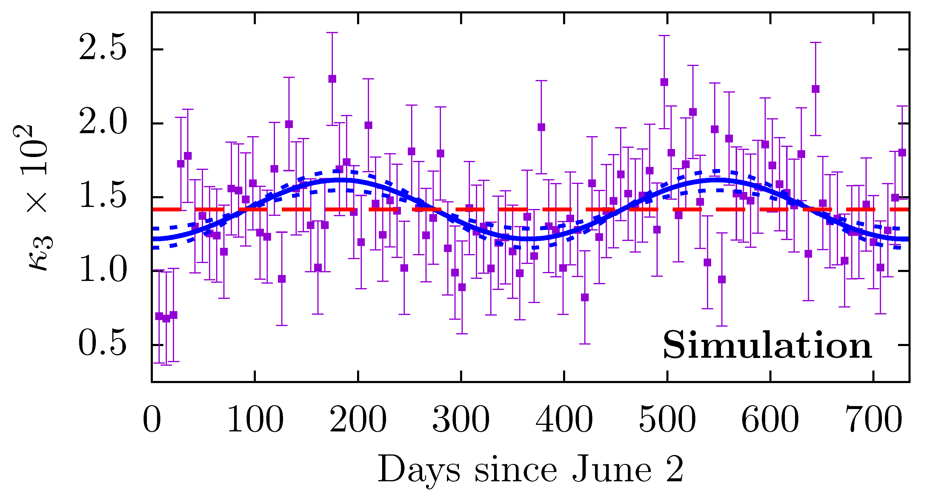
2.5. Annual Modulation
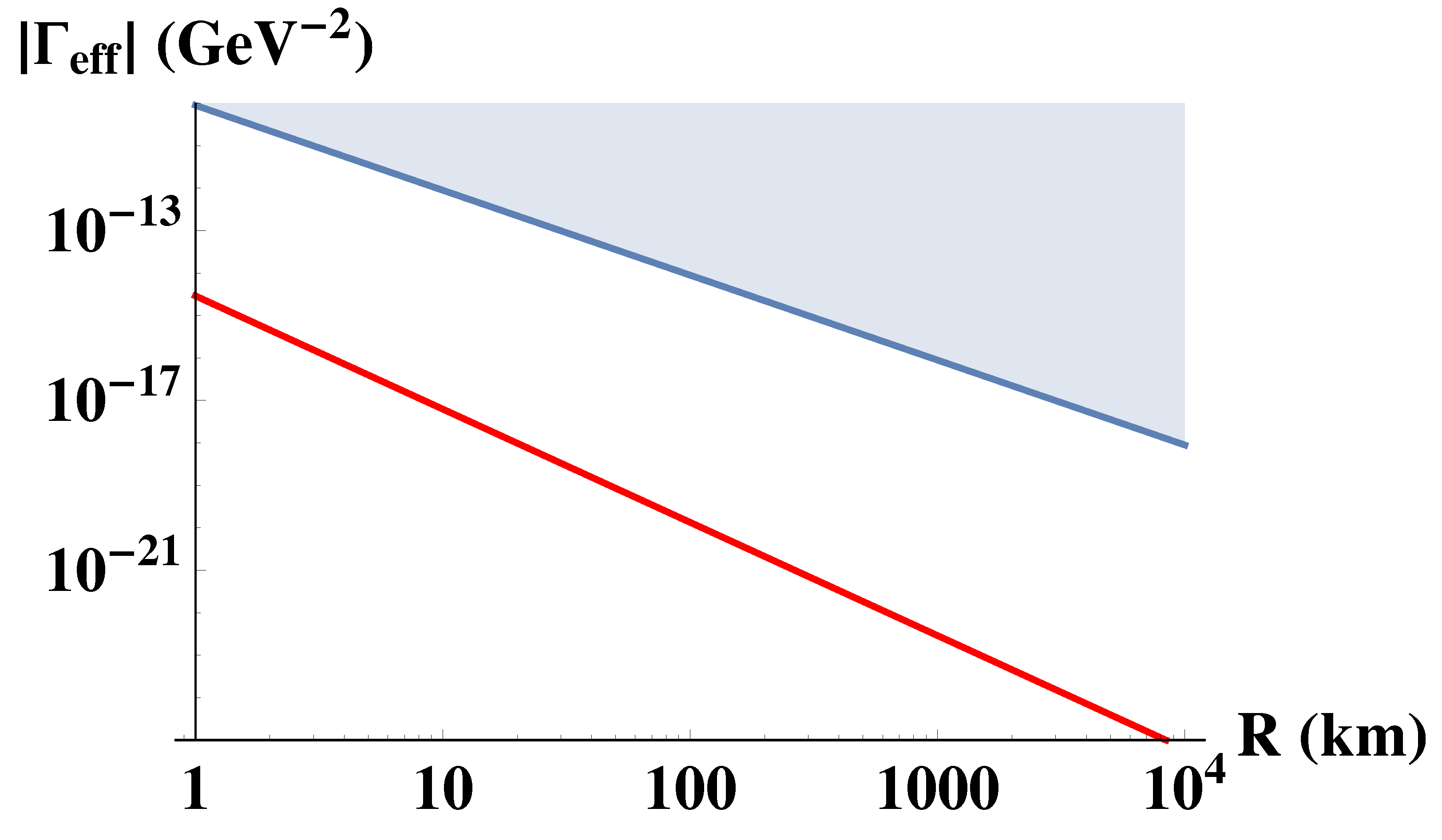
As the Earth orbits the Sun, there is an annual modulation in the addition of their velocities. This causes an annual modulation in the Earth’s velocity relative to the galactic DM halo, and hence to the mean DM encounter rate. We may therefore express the rate, R = 1 / T , as
R ( t ) = R ( 0 ) 1 + Δ v v g cos ( Ω t + φ ) ,
where Ω = 2 π / yr , φ is the phase with Ω t + φ = 0 on 2 June, and Δ v / v g 0.05 [30].
Then, the skewness (and other moments) becomes time-dependent:
κ 3 ( t ) κ 3 ( 0 ) κ 3 ( m ) cos ( Ω t + φ ) .
The DM-induced skewness (14) scales linearly with the rate, and as the cube of the mean signal magnitude. The mean signal magnitude scales inversely with velocity (11). Therefore, the modulation amplitude is
κ 3 ( m ) = 2 Δ v v 0 κ 3 10 % .
We demonstrate this using simulated data in Figure 2. Similarly, the annual modulation in the kurtosis is
κ 4 ( m ) = 3 Δ v v 0 κ 3 15 % .
If the data are divided into M time bins, each consisting of N M = N / M points, with the skewness calculated for each bin, the modulation amplitude can be extracted as
κ 3 ( m ) = 2 | κ ˜ 3 ( 1 / yr ) | M ± δ κ 3 ( m ) ,
where κ ˜ 3 is the Fourier transform of κ 3 ( t ) . The sample uncertainty, δ κ 3 ( m ) 2 6 / N , is independent of the number of bins. However, the requirement to have several encounters per bin limits the sensitivity region to T N M τ 0 = T obs / M .
To detect the annual modulation in the skewness, we require that κ 3 ( m ) > δ κ 3 ( m ) . This implies that we require signals with combination χ 0 3 / T that are larger by a factor v / Δ v 20 compared to the result for the mean skewness (15). Or, for a fixed value of T , signals that are ∼3 times larger. Nevertheless, it is important that there are signatures unique to DM (namely, the modulation phase, period, and amplitude) that can be sought in such experiments. If a skewness is present in the data, one may exclude DM origins if the modulation is absent.

3. Discussion

As an illustrative example, we analyze six years of archival atomic clock data [63,64] from the comparison of several Cs GPS satellite clocks to an Earth-based H-maser. We use the same GPS data used by us in Ref. [42]; see Refs. [33,42] for a description of the GPS clock data relevant to the analysis. The calculated skewness in the clock-comparison residuals is
κ 3 ( Cs ) = ( 0.1 ± 47.0 ) × 10 3 ,
which, at the 68% confidence level, implies | κ 3 | < 4.7 × 10 2 (for this GPS data, σ 0.09 ns , and τ 0 = 30 s [32]). The uncertainty in κ 3 was found by calculating the skewness for each day of data separately; note that this is larger than the assumed sample skewness due to the presence of non-Gaussian noise (including outliers, which are not removed) in the data. From Equation (16), we can thus place constraints on the Γ X couplings. Importantly, this allows one to place constraints on couplings for macroscopic DM objects with radii R < 10 4 km , the region that is otherwise inaccessible using global network methods [32].
To demonstrate this in more concrete terms, we assume here a scalar field DM model for which the energy density inside the DM objects scales as ρ ϕ ϕ 0 2 m ϕ 2 , and the size of the objects is set by the Compton wavelength R ħ / m ϕ c . This is consistent, for example, with topological defect models [11] (we note however, that this is just an example, and for other models, different relations will hold). In this case, if no signal is observed, the model may be constrained as
| Γ eff | R 2 < σ | κ 3 max | 1 / 3 ħ c ρ DM T 2 / 3 τ 0 1 / 3 .
Preliminary results for such a model from the above analysis of the Cs GPS clocks is presented in Figure 3. Note that results from the experiments in Refs. [41,42,44,46] do not apply in the considered parameter range. Shown also is the projected sensitivity for 1 year of data from an optical Sr clock, assuming σ 10 16 s at averaging time of τ 0 = 1 s . Such clocks have been used recently for DM searches, both for “clumpy” and oscillating DM models, in Refs. [44,46]; details of the clock performance are given in those works (see also discussion of clock servo loop and averaging times relevant to DM searches in Refs. [42,46]). This projection takes into account that the optimal averaging time to use when searching for DM objects of radius R is τ avg R / v g .
The results of our analysis for the quadratic portal (4) can be easily translated into the constraints on the derivative portal () by noticing that ( μ ϕ ) ( μ ϕ * ) | ϕ | 2 , where we neglected the time derivative because of the non-relativistic nature of cold DM. Further, for a Gaussian-profiled “blob” | ϕ | 2 ϕ 0 2 / R 2 . Thereby,
Γ X Γ X R 2 / ( ħ c ) 2
and the constraint (25) translates into
| Γ eff | < σ | κ 3 max | 1 / 3 ( ħ c ) 3 ρ DM T 2 / 3 τ 0 1 / 3 .
Can our DM observable, the noise asymmetry, be mimicked by fluctuations in DM energy density, ρ DM ? It can not. Indeed, the sign of the frequency perturbation (7) due to a single DM blob is fixed. DM energy density (or the number density of DM blobs) affects the encounter rate of DM blobs with the sensor. However, since the sign of the DM-induced perturbation remains the same, all individual perturbations add coherently. If DM energy density fluctuates, it would only scale the DM blob flux and thus the observable.
Another relevant point recently raised in the literature [65] is the effect of DM energy density fluctuations on the coupling strength constraints. For scalar fields, the effective sensitivity was shown to be reduced by a factor of a few. Considering the logarithmic scale of Figure 3 and the preliminary, illustrative nature of our results, this corrective factor would not affect our conclusions.

4. Conclusions

In this work, we proposed a new dark matter signature: an asymmetry (and other non-Gaussianities) that may be induced in the noise distributions of precision quantum sensors, such as atomic clocks. Such signatures may be induced by dark matter candidates composed of self-interacting ultralight quantum fields that form macroscopic objects, examples of which include Q-balls and topological defects. Further, we demonstrate that there would be a sizeable annual modulation in these signatures due to the annual variation of the Earth velocity with respect to dark matter halo. As an application of our formalism, we use 6 years of data from the atomic clocks on board GPS satellites to place constraints on a scalar dark matter model, and show projections for future experiments based on laboratory clocks. This technique allows one to search for DM models that would otherwise be undetectable using existing experiments.

Author Contributions

Conceptualization, A.D. and B.M.R.; methodology, A.D. and B.M.R.; software, B.M.R..; writing—original draft preparation, B.M.R.; writing—review and editing, B.M.R. and A.D; visualization, B.M.R.; supervision, A.D.; project administration, A.D.; funding acquisition, A.D. All authors have read and agreed to the published version of the manuscript.

Funding

This work was supported in part by the U.S. National Science Foundation grants PHY-1912465 and PHY-1806672 and by the Australian Research Council.

Institutional Review Board Statement

Not applicable.

Informed Consent Statement

Not applicable.

Data Availability Statement

Publicly available datasets were analyzed in this study. This data can be found here: ftp://sideshow.jpl.nasa.gov/pub/jpligsac/ (accessed on 27 February 2021).

Conflicts of Interest

The authors declare no conflict of interest. The funders had no role in the design of the study; in the collection, analyses, or interpretation of data; in the writing of the manuscript, or in the decision to publish the results.

Abbreviations

The following abbreviations are used in this manuscript:
WIMPweakly-interacting massive particle
DMdark matter
GPSGlobal Positioning System

References

  1. Weinberg, S. Cosmology; Cosmology, Oxford University Press: New York, NY, USA, 2008. [Google Scholar]
  2. Peebles, P.J.E. The cosmological constant and dark energy. Rev. Mod. Phys. 2003, 75, 559–606. [Google Scholar] [CrossRef] [Green Version]
  3. Bertone, G.; Hooper, D.; Silk, J. Particle dark matter: Evidence, candidates and constraints. Phys. Rep. 2005, 405, 279–390. [Google Scholar] [CrossRef] [Green Version]
  4. Feng, J.L. Dark Matter Candidates from Particle Physics and Methods of Detection. Ann. Rev. Astron. Astrophys. 2010, 48, 495–545. [Google Scholar] [CrossRef] [Green Version]
  5. Matarrese, S.; Colpi, M.; Gorini, V.; Moschella, U. Dark Matter and Dark Energy: A Challenge for Modern Cosmology; Springer: Berlin/Heidelberg, Germany, 2011. [Google Scholar]
  6. Blumenthal, G.R.; Faber, S.M.; Primack, J.R.; Rees, M.J. Formation of galaxies and large-scale structure with cold dark matter. Nature 1984, 311, 517–525. [Google Scholar] [CrossRef]
  7. The XENON Collaboration. First Dark Matter Search Results from the XENON1T Experiment. Phys. Rev. Lett. 2017, 119, 181301. [Google Scholar] [CrossRef] [Green Version]
  8. Liu, J.; Chen, X.; Ji, X. Current status of direct dark matter detection experiments. Nat. Phys. 2017, 13, 212–216. [Google Scholar] [CrossRef]
  9. Bertone, G.; Tait, T.M.P. A new era in the search for dark matter. Nature 2018, 562, 51–56. [Google Scholar] [CrossRef] [Green Version]
  10. Berezinsky, V.S.; Dokuchaev, V.I.; Eroshenko, Y.N. Small-scale clumps of dark matter. Phys. Uspekhi 2014, 57, 1–36. [Google Scholar] [CrossRef] [Green Version]
  11. Derevianko, A.; Pospelov, M. Hunting for topological dark matter with atomic clocks. Nat. Phys. 2014, 10, 933–936. [Google Scholar] [CrossRef] [Green Version]
  12. Safronova, M.S.; Budker, D.; DeMille, D.; Kimball, D.F.J.; Derevianko, A.; Clark, C.W. Search for new physics with atoms and molecules. Rev. Mod. Phys. 2018, 90, 025008. [Google Scholar] [CrossRef] [Green Version]
  13. Coleman, S. Q-balls. Nucl. Phys. B 1985, 262, 263–283. [Google Scholar] [CrossRef]
  14. Lee, T.D. Soliton stars and the critical masses of black holes. Phys. Rev. D 1987, 35, 3637–3639. [Google Scholar] [CrossRef] [PubMed]
  15. Kusenko, A.; Steinhardt, P.J. Q-ball candidates for self-interacting dark matter. Phys. Rev. Lett. 2001, 87, 141301. [Google Scholar] [CrossRef] [PubMed] [Green Version]
  16. Kimball, D.F.J.; Budker, D.; Eby, J.; Pospelov, M.; Pustelny, S.; Scholtes, T.; Stadnik, Y.V.; Weis, A.; Wickenbrock, A. Searching for axion stars and Q-balls with a terrestrial magnetometer network. Phys. Rev. D 2018, 97, 043002. [Google Scholar] [CrossRef] [Green Version]
  17. Hogan, C.J.; Rees, M.J. Axion miniclusters. Phys. Lett. B 1988, 205, 228–230. [Google Scholar] [CrossRef]
  18. Barranco, J.; Monteverde, A.C.; Delepine, D. Can the dark matter halo be a collisionless ensemble of axion stars? Phys. Rev. D 2013, 87, 103011. [Google Scholar] [CrossRef] [Green Version]
  19. Krippendorf, S.; Muia, F.; Quevedo, F. Moduli stars. J. High Energy Phys. 2018, 2018, 70. [Google Scholar] [CrossRef] [Green Version]
  20. Kibble, T. Some Implications of a Cosmological Phase Transition. Phys. Rep. 1980, 67, 183–199. [Google Scholar] [CrossRef]
  21. Vilenkin, A. Cosmic strings and domain walls. Phys. Rep. 1985, 121, 263–315. [Google Scholar] [CrossRef]
  22. Vilenkin, A.; Shaposhnikov, M. Cosmic Strings and Other Topological Defects; Cambridge University Press: Cambridge, UK, 1994. [Google Scholar]
  23. Ge, S.; Lawson, K.; Zhitnitsky, A. Axion quark nugget dark matter model: Size distribution and survival pattern. Phys. Rev. D 2019, 99, 116017. [Google Scholar] [CrossRef] [Green Version]
  24. Budker, D.; Flambaum, V.V.; Liang, X.; Zhitnitsky, A. Axion quark nuggets and how a global network can discover them. Phys. Rev. D 2020, 101, 043012. [Google Scholar] [CrossRef] [Green Version]
  25. Budker, D.; Flambaum, V.V.; Zhitnitsky, A. Axion Quark Nuggets. SkyQuakes and Other Mysterious Explosions. arXiv preprint 2020, arXiv:2003.07363. [Google Scholar]
  26. Grabowska, D.M.; Melia, T.; Rajendran, S. Detecting dark blobs. Phys. Rev. D 2018, 98, 115020. [Google Scholar] [CrossRef] [Green Version]
  27. Brax, P.; Valageas, P.; Cembranos, J.A. Nonrelativistic formation of scalar clumps as a candidate for dark matter. Phys. Rev. D 2020, 102, 22–35. [Google Scholar] [CrossRef]
  28. Niikura, H.; Takada, M.; Yasuda, N.; Lupton, R.H.; Sumi, T.; More, S.; Kurita, T.; Sugiyama, S.; More, A.; Oguri, M.; et al. Microlensing constraints on primordial black holes with Subaru/HSC Andromeda observations. Nat. Astron. 2019, 3, 524–534. [Google Scholar] [CrossRef]
  29. Nesti, F.; Salucci, P. The Dark Matter halo of the Milky Way, AD 2013. J. Cosmol. Astropart. Phys. 2013, 2013, 16. [Google Scholar] [CrossRef]
  30. Freese, K.; Lisanti, M.; Savage, C. Colloquium: Annual modulation of dark matter. Rev. Mod. Phys. 2013, 85, 1561–1581. [Google Scholar] [CrossRef] [Green Version]
  31. Pospelov, M.; Pustelny, S.; Ledbetter, M.P.; Kimball, D.F.J.; Gawlik, W.; Budker, D. Detecting domain walls of axionlike models using terrestrial experiments. Phys. Rev. Lett. 2013, 110, 021803. [Google Scholar] [CrossRef]
  32. Roberts, B.M.; Blewitt, G.; Dailey, C.; Derevianko, A. Search for transient ultralight dark matter signatures with networks of precision measurement devices using a Bayesian statistics method. Phys. Rev. D 2018, 97, 083009. [Google Scholar] [CrossRef] [Green Version]
  33. Panelli, G.; Roberts, B.M.; Derevianko, A. Applying the matched-filter technique to the search for dark matter transients with networks of quantum sensors. EPJ Quantum Technol. 2020, 7, 5. [Google Scholar] [CrossRef] [Green Version]
  34. Masia-Roig, H.; Smiga, J.A.; Budker, D.; Dumont, V.; Grujic, Z.; Kim, D.; Jackson Kimball, D.F.; Lebedev, V.; Monroy, M.; Pustelny, S.; et al. Analysis method for detecting topological defect dark matter with a global magnetometer network. Phys. Dark Universe 2020, 28, 100494. [Google Scholar] [CrossRef] [Green Version]
  35. Jaeckel, J.; Schenk, S.; Spannowsky, M. Probing Dark Matter Clumps, Strings and Domain Walls with Gravitational Wave Detectors. arXiv preprint 2020, arXiv:2004.13724. [Google Scholar]
  36. Dailey, C.; Bradley, C.; Jackson Kimball, D.F.; Sulai, I.A.; Pustelny, S.; Wickenbrock, A.; Derevianko, A. Quantum sensor networks as exotic field telescopes for multi-messenger astronomy. Nat. Astron. 2020. [Google Scholar] [CrossRef]
  37. The LIGO Scientific Collaboration and Virgo Collaboration. Observation of Gravitational Waves from a Binary Black Hole Merger. Phys. Rev. Lett. 2016, 116, 061102. [Google Scholar] [CrossRef] [PubMed]
  38. Arvanitaki, A.; Huang, J.; Van Tilburg, K. Searching for dilaton dark matter with atomic clocks. Phys. Rev. D 2015, 91, 015015. [Google Scholar] [CrossRef] [Green Version]
  39. Van Tilburg, K.; Leefer, N.; Bougas, L.; Budker, D. Search for Ultralight Scalar Dark Matter with Atomic Spectroscopy. Phys. Rev. Lett. 2015, 115, 011802. [Google Scholar] [CrossRef]
  40. Hees, A.; Guéna, J.; Abgrall, M.; Bize, S.; Wolf, P. Searching for an Oscillating Massive Scalar Field as a Dark Matter Candidate Using Atomic Hyperfine Frequency Comparisons. Phys. Rev. Lett. 2016, 117, 061301. [Google Scholar] [CrossRef]
  41. Wcisło, P.; Morzyński, P.; Bober, M.; Cygan, A.; Lisak, D.; Ciuryło, R.; Zawada, M. Experimental constraint on dark matter detection with optical atomic clocks. Nat. Astron. 2016, 1, 0009. [Google Scholar] [CrossRef]
  42. Roberts, B.M.; Blewitt, G.; Dailey, C.; Murphy, M.; Pospelov, M.; Rollings, A.; Sherman, J.; Williams, W.; Derevianko, A. Search for domain wall dark matter with atomic clocks on board global positioning system satellites. Nat. Commun. 2017, 8, 1195. [Google Scholar] [CrossRef] [PubMed]
  43. Kalaydzhyan, T.; Yu, N. Extracting dark matter signatures from atomic clock stability measurements. Phys. Rev. D 2017, 96, 075007. [Google Scholar] [CrossRef] [Green Version]
  44. Wcislo, P.; Ablewski, P.; Beloy, K.; Bilicki, S.; Bober, M.; Brown, R.; Fasano, R.; Ciurylo, R.; Hachisu, H.; Ido, T.; et al. New bounds on dark matter coupling from a global network of optical atomic clocks. Sci. Adv. 2018, 4, eaau4869. [Google Scholar] [CrossRef] [Green Version]
  45. Savalle, E.; Hees, A.; Frank, F.; Cantin, E.; Pottie, P.E.; Roberts, B.M.; Cros, L.; McAllister, B.T.; Wolf, P. Searching for DArk Matter with a Non-Equal Delay inteferometer: The DAMNED experiment. Phys. Rev. Lett. 2021, accepted. [Google Scholar]
  46. Roberts, B.M.; Delva, P.; Al-Masoudi, A.; Amy-Klein, A.; Bærentsen, C.; Baynham, C.F.A.; Benkler, E.; Bilicki, S.; Bize, S.; Bowden, W.; et al. Search for transient variations of the fine structure constant and dark matter using fiber-linked optical atomic clocks. New J. Phys. 2020, 22, 093010. [Google Scholar] [CrossRef]
  47. Stadnik, Y.V.; Flambaum, V.V. Searching for dark matter and variation of fundamental constants with laser and maser interferometry. Phys. Rev. Lett. 2015, 114, 161301. [Google Scholar] [CrossRef] [PubMed] [Green Version]
  48. Stadnik, Y.V.; Flambaum, V.V. Enhanced effects of variation of the fundamental constants in laser interferometers and application to dark-matter detection. Phys. Rev. A 2016, 93, 063630. [Google Scholar] [CrossRef] [Green Version]
  49. Arvanitaki, A.; Graham, P.W.; Hogan, J.M.; Rajendran, S.; Van Tilburg, K. Search for light scalar dark matter with atomic gravitational wave detectors. Phys. Rev. D 2018, 97, 075020. [Google Scholar] [CrossRef] [Green Version]
  50. Hu, W.; Lawson, M.; Budker, D.; Figueroa, N.L.; Kimball, D.F.J.; Mills, A.P.; Voigt, C. A network of precision gravimeters as a detector of matter with feeble nongravitational coupling. Eur. Phys. J. D 2020, 74, 115. [Google Scholar] [CrossRef]
  51. McNally, R.L.; Zelevinsky, T. Constraining domain wall dark matter with a network of superconducting gravimeters and LIGO. Eur. Phys. J. D 2020, 74, 61. [Google Scholar] [CrossRef]
  52. Savalle, E.; Roberts, B.M.; Frank, F.; Pottie, P.E.; McAllister, B.T.; Dailey, C.; Derevianko, A.; Wolf, P. Novel approaches to dark-matter detection using space-time separated clocks. arXiv preprint 2019, arXiv:1902.07192. [Google Scholar]
  53. Baron, J.; Campbell, W.C.; DeMille, D.; Doyle, J.M.; Gabrielse, G.; Gurevich, Y.V.; Hess, P.W.; Hutzler, N.R.; Kirilov, E.; Kozyryev, I.; et al. Order of magnitude smaller limit on the electric dipole moment of the electron. Science 2014, 343, 269–272. [Google Scholar] [CrossRef] [Green Version]
  54. Roberts, B.M.; Stadnik, Y.V.; Dzuba, V.A.; Flambaum, V.V.; Leefer, N.; Budker, D. Parity-violating interactions of cosmic fields with atoms, molecules, and nuclei: Concepts and calculations for laboratory searches and extracting limits. Phys. Rev. D 2014, 90, 096005. [Google Scholar] [CrossRef] [Green Version]
  55. Roberts, B.M.; Stadnik, Y.V.; Dzuba, V.A.; Flambaum, V.V.; Leefer, N.; Budker, D. Limiting P-Odd Interactions of Cosmic Fields with Electrons, Protons, and Neutrons. Phys. Rev. Lett. 2014, 113, 81601. [Google Scholar] [CrossRef] [Green Version]
  56. Abel, C.; Ayres, N.J.; Ban, G.; Bison, G.; Bodek, K.; Bondar, V.; Daum, M.; Fairbairn, M.; Flambaum, V.V.; Geltenbort, P.; et al. Search for Axionlike Dark Matter through Nuclear Spin Precession in Electric and Magnetic Fields. Phys. Rev. X 2017, 7, 041034. [Google Scholar] [CrossRef] [Green Version]
  57. Bovy, J.; Tremaine, S. On the local dark matter density. Astrophys. J. 2012, 756, 89. [Google Scholar] [CrossRef]
  58. Hernández, X.; Matos, T.; Sussman, R.A.; Verbin, Y. Scalar field “mini-MACHOs”: A new explanation for galactic dark matter. Phys. Rev. D 2004, 70, 043537. [Google Scholar] [CrossRef] [Green Version]
  59. González-Morales, A.X.; Valenzuela, O.; Aguilar, L.A. Constraining dark matter sub-structure with the dynamics of astrophysical systems. J. Cosmol. Astropart. Phys. 2013, 2013, 001. [Google Scholar] [CrossRef] [Green Version]
  60. Angstmann, E.J.; Dzuba, V.A.; Flambaum, V.V. Relativistic effects in two valence-electron atoms and ions and the search for variation of the fine-structure constant. Phys. Rev. A 2004, 70, 014102. [Google Scholar] [CrossRef] [Green Version]
  61. Dinh, T.H.; Dunning, A.; Dzuba, V.A.; Flambaum, V.V. Sensitivity of hyperfine structure to nuclear radius and quark mass variation. Phys. Rev. A 2009, 79, 054102. [Google Scholar] [CrossRef] [Green Version]
  62. Roberts, B.M. Companion Code 2018. Available online: https://github.com/benroberts999/DM-ClockAsymmetry (accessed on 27 February 2021).
  63. Jet Propulsion Laboratory. Available online: ftp://sideshow.jpl.nasa.gov/pub/jpligsac/ (accessed on 27 February 2021).
  64. Jean, Y.; Dach, R. International GNSS Service Technical Report 2015 (IGS Annual Report); IGS Central Bureau and University of Bern, Bern Open Publishing: Bern, Switzerland, 2016. [Google Scholar] [CrossRef]
  65. Centers, G.P.; Blanchard, J.W.; Conrad, J.; Figueroa, N.L.; Garcon, A.; Gramolin, A.V.; Kimball, D.F.J.; Lawson, M.; Pelssers, B.; Smiga, J.A.; et al. Stochastic amplitude fluctuations of bosonic dark matter and revised constraints on linear couplings. arXiv preprint 2019, arXiv:1905.13650. [Google Scholar]
Figure 1. DM objects incident upon the Earth, and the induced shift and asymmetry in the clock noise distribution.
Universe 07 00050 g001
Figure 2. Simulation for two years of data ( τ 0 = 1 s), with DM signals ( R 0 τ 0 = 0.01 , χ 0 / σ = 1 ) including the annual velocity modulation [62]. The skewness is calculated for each week of data (purple squares, with 6 / N error bars). The extracted modulation amplitude is κ 3 ( m ) = 0.2 × 10 2 (23). The solid blue curve is the best-fit cosine, and the dotted lines are the uncertainties. The dashed red curve shows the mean κ 3 .
Universe 07 00050 g002
Figure 3. Preliminary results: constraints on a general scalar “DM blob” model with quadratic interactions as per Equation (7), for the average time between encounter T = 1 day. The shaded blue region is the preliminary constraints found in this work from six years of data from the Cs GPS clocks. The red line shows the potential discovery reach for one year of data from a single laboratory optical Sr clock as described in the text. These constraints can be easily rescaled into those for a derivative portal coupling strengths via Equation (26).
Universe 07 00050 g003
Publisher’s Note: MDPI stays neutral with regard to jurisdictional claims in published maps and institutional affiliations.

