Stellar Chromospheric Variability

Abstract

Cool stars with convective envelopes of spectral types F and later tend to exhibit magnetic activity throughout their atmospheres. The presence of strong and variable magnetic fields is evidenced by photospheric starspots, chromospheric plages and coronal flares, as well as by strong Ca ii H+K and H$\alpha$ emission, combined with the presence of ultraviolet resonance lines. We review the drivers of stellar chromospheric activity and the resulting physical parameters implied by the observational diagnostics. At a basic level, we explore the importance of stellar dynamos and their activity cycles for a range of stellar types across the Hertzsprung–Russell diagram. We focus, in particular, on recent developments pertaining to stellar rotation properties, including the putative Vaughan–Preston gap. We also pay specific attention to magnetic variability associated with close binary systems, including RS Canum Venaticorum, BY Draconis, W Ursae Majoris and Algol binaries. At the present time, large-scale photometric and spectroscopic surveys are becoming generally available, thus leading to a resurgence of research into chromospheric activity. This opens up promising prospects to gain a much improved understanding of chromospheric physics and its wide-ranging impact.

1. Introduction

Stellar atmospheres are composed of several distinct layers. In solar-type stars, the innermost atmospheric layer, the photosphere, is located just above the surface convection zone (see Figure 1). The latter is an unstable layer where plasma circulates between the stellar interior and its surface layers because of the plasma’s temperature-dependent buoyant properties. The Sun’s photosphere, the layer from which light is emitted, represents a radial shell with a width on the order of 100 km. At larger radii, the next main solar atmospheric zone is the chromosphere (‘sphere of colour’), covering altitudes of approximately 3000–5000 km and extending through a region of partial hydrogen ionisation. Almost all luminous stars, except for white dwarfs, feature chromospheres of some sort, although they are usually most prominent and magnetically active in lower main-sequence stars and brown dwarfs of F and later spectral types, as well as in giant and subgiant stars.

For earlier-type, hotter stars, which are dominated by radiative rather than convective processes at their surfaces, the disappearance of a convective envelope at the stellar surface implies the disappearance of a solar-like magnetised chromosphere. Magnetised stellar chromospheres may not be strictly equivalent to the solar chromosphere, however. Stellar atmospheric zones commonly referred to as chromospheres have also been detected in giant and supergiant stars in globular clusters and the general field stellar populations in both the Milky Way and the Magellanic Clouds [1,2,3,4,5,6,7,8].

Chromospheres exhibit temperature inversion. The temperature of the solar chromosphere initially cools down from the Sun’s surface temperature of about 5770–5780 K to approximately 3840 K in the ‘temperature minimum region’ (see Figure 2). It then rapidly increases to temperatures in excess of 35,000 K at the onset of the solar atmospheric transition region, which extends to the corona [9,10]. Figure 2 is a schematic representation of the solar atmosphere, showing the dependence of temperature and density on height above the surface. Heating of the chromosphere to temperatures above the level required to maintain radiative equilibrium is driven by a combination of mechanical heating (pulsations and shocks), acoustic heating (pulsation-driven sound waves causing hydrodynamic shocks), magnetic fields (Alfvén waves, i.e., transverse or torsional magnetohydrodynamic waves), turbulence and ambipolar diffusion ([11,12,13,14,15,16], and references therein)—i.e., separation (at the same rate) of oppositely charged species in a plasma owing to the effects of the ambient electric field.

Chromospheric heating processes have been scrutinised at least since Biermann [17]—whose explanation evolved into the standard heating theory—and Parker [18,19]; they are still subject to intense debate (e.g., [20]). A detailed discussion of these heating processes is well beyond the scope of this review, however. Instead, we refer the interested reader to the comprehensive review recently published by Srivastava et al. [16].

Most importantly, in the solar chromosphere magnetic heating causes the temperature to increase to a plateau of approximately 7000 K, with the ambient density falling by orders of magnitude with respect to the region near the photosphere (see Figure 2) [20,21]. The 7000 K plateau results from a balance between magnetic heating and radiative cooling through collisionally excited H$\alpha$, Ca ii K and Mg ii k radiation. The latter lines are the principal diagnostic lines formed in the chromosphere (for details, see Section 3). Their intensity scales with the level of non-thermal heating in the chromosphere, so that they are useful proxies for both the strength of the underlying magnetic field and the area covered by that field. At higher altitudes in the chromosphere and into the corona beyond, the density becomes too tenuous for collisional heating by electrons from ionised hydrogen to continue to play any role of importance, with the low density also rendering cooling inefficient.

At its base, the chromosphere is homogeneous, although numerous filaments and ‘spicules’ extend up to altitudes of several $\times {10}^4$ km. Some even reach up to some 150,000 km in the form of the solar prominences (filaments viewed side-on) associated with coronal mass ejections. Both filaments and spicules—as well as their horizontal counterparts, known as ‘fibrils’—are plumes and tendrils of luminous gas. Their presence reflects the importance of magnetic activity, e.g., organised in the form of magnetic flux tubes [22]. As we will see in Section 2.2.1, the magnetic field is organised in flux tubes because of the prevailing balance between a local negative pressure gradient, $B^2/8\pi$ (where B is the local magnetic field vector), and a local tension component.

Figure 2. Temperature (solid line) and density (dashed line) as a function of height above the top of the photosphere in the solar atmosphere ([23], p. 2; courtesy: NASA). Yellow and orange peaks are chromospheric spicules that protrude into the corona. The transition region between the chromosphere and the corona is shown as a dark yellow band, only a few hundred kilometres thick, which follows the spicule outlines.

Figure 2. Temperature (solid line) and density (dashed line) as a function of height above the top of the photosphere in the solar atmosphere ([23], p. 2; courtesy: NASA). Yellow and orange peaks are chromospheric spicules that protrude into the corona. The transition region between the chromosphere and the corona is shown as a dark yellow band, only a few hundred kilometres thick, which follows the spicule outlines.

Chromospheric (magnetic) activity is related to photometric and spectroscopic variability on a range of timescales. Day- to year-long variability is associated with the evolution and rotational modulation of individual magnetically active regions. That is, stellar rotation is intricately correlated with chromospheric activity, as well as with stellar age (see Section 3.3). In fact, stellar rotation—particularly differential rotation—is responsible for the conversion of undisturbed poloidal magnetic fields into twisted toroidal fields (see Section 2.2.3) (e.g., [24]). Long-term chromospheric activity, characterised by timescales on the order of years to centuries, is thought to be driven by the same physical principles as the stellar (and solar) dynamo (see Section 2.2). The underlying physics is highly complex.

Magnetic activity is likely triggered by the interplay of rotation and turbulent convection at the stellar surface. In turn, this triggers cyclic and self-sustained global stellar magnetic activity, including the well-known 11-year solar sunspot activity cycle [25,26]. Direct solar observations have been performed since approximately 1609. This wealth of observational data has allowed us to explore the significant variability of the Sun’s cycle-averaged magnetic activity level in great detail. The latter ranges from the extremely quiet ‘Maunder Minimum’ (1645–1715), when photospheric sunspots almost completely disappeared, to the present-day enhanced magnetic activity. The Maunder Minimum is a representative ‘Grand Minimum’ of solar magnetic activity [27], corresponding to a special, as yet poorly understood state of the solar dynamo (e.g., see Section 2.2.1) [28,29]. Despite a dearth of sunspots during the Maunder Minimum, the solar wind remained active, although at a reduced level [30,31].

With increasing stellar age, the strength of the surface magnetic field—and, hence, a star’s magnetic activity—decreases in response to magnetic braking of a star’s rotation rate through angular momentum losses induced by magnetised winds and structural variations [32,33]. As such, quantification of a star’s chromospheric magnetic activity offers a direct stellar age measurement [26,34,35,36,37,38,39,40,41]: see Section 3, specifically Section 3.3. More broadly, a tightly constrained chromospheric activity–age correlation offers direct insights into the properties of exoplanet host stars and Galactic chemodynamical evolution scenarios. In addition, chromospheric activity relates the changes observed at the stellar surface to changes occurring deeper into the stellar interior [42], e.g., in the context of non-convective mixing of abundances in advanced evolutionary stages, in particular for stars exhibiting solar-like dynamos ([43,44], and references therein). Hence, its study can shed light on the physical mechanisms responsible for these changes [45,46] and thus better constrain dynamo models [47,48]: see Section 2.2.

Finally, magnetically active stars tend to exhibit flares or superflares (sudden releases of magnetic energy) [49], often large and rapidly evolving starspots (cooler regions where convection is suppressed by strong magnetic fields) [50,51,52,53,54], as well as faculae and plages (unusually bright regions in the photosphere and chromosphere, respectively) [8,55]. Dark starspots and bright faculae are usually located in stellar photospheres, whereas plages tend to be associated with chromospheres [55]. Chromospheric and photospheric magnetic activity in general, and flares in particular, may have an impact on planetary habitability [56,57,58], both in the solar system and in exoplanetary systems, which is of potential importance in the context of the Earth’s climatological evolution and the solar–terrestrial connection.

Here, we review recent developments and advances in our understanding of stellar chromospheric activity, including for the Sun. Although our focus is predominantly on new observational insights, we will first cover the basic theory of stellar dynamos, with specific emphasis on the solar dynamo (Section 2.2). We have aimed to compose an intermediate-length review suitable as a graduate-level entry point into this active area of contemporary research. We have made the conscious choice to limit our coverage of stellar atmospheric physics outside the chromosphere, and we only cover the underlying theory in a rudimentary manner. For more in-depth discussions of aspects that are tangential to the principal aims of this review, we have included extensive referencing. We note that it is not our aim to provide a full overview of the field of solar physics. Instead, we treat the Sun as an example of a chromospherically moderately active G-type star whose fortuitous proximity allows us to explore certain aspects in much more detail than would be possible for more distant objects.

Following a high-level overview of the theory of stellar dynamo physics, we will discuss the broad range of observational diagnostics employed to trace and understand stellar chromospheric activity and variability: see Section 3. In Section 4 and Section 5 we discuss the extant body of observational evidence pertaining to the level of chromospheric activity as a function of spectral type and in close binary systems, respectively, before concluding this review in Section 6, where we summarise current trends and provide a future outlook.

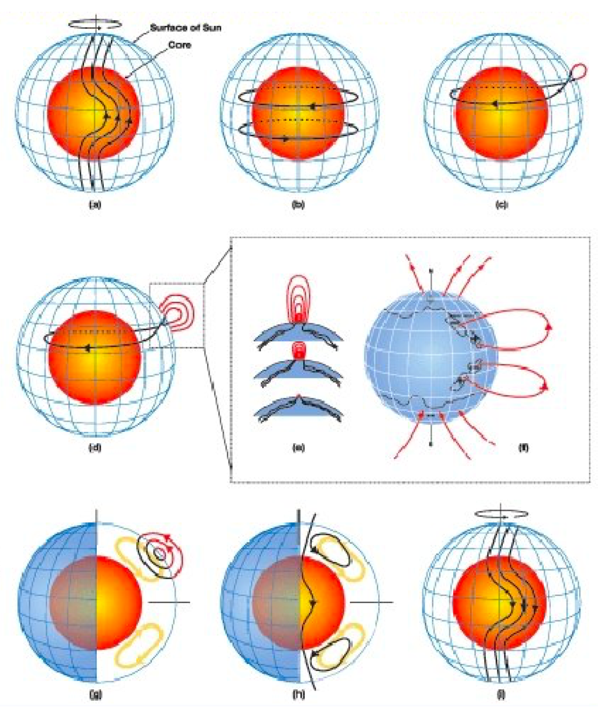
2. Magnetic Activity Cycles and the Solar Dynamo

Studying the Sun’s magnetism in the context of other stars offers a gateway to studying magnetic activity in cool stars and understanding the stellar dynamo and its relationship with stellar properties.

2.1. The Solar Activity Cycle

The Sun is a middle-aged G-type star. It is a magnetically moderately active star exhibiting short- to long-term fluctuations ranging from a fraction of a second to billions of years. Through the pioneering work of George Ellery Hale and his collaborators in the early 1900s, it was established that the Sun’s magnetic nature drives solar activity (i.e., solar flares, coronal mass ejections, high-speed solar winds and solar energetic particles) and, in particular, the presence and appearance of sunspots. Hale’s polarity laws established the presence of a magnetic flux system in the interior of the Sun as a source of sunspots. The origin of the magnetic field was initially attributed to the inductive action of fluid motions [59]. The hypothesis proposed by Larmor [59] suggested that the axisymmetric and equatorially symmetric differential rotation pervading the solar interior caused shearing of a large-scale poloidal magnetic field, resulting in the inferred equatorial antisymmetry of the internal solar toroidal fields. Although this theory held its ground for two decades, Cowling’s antidynamo theorem [60] had already demonstrated that even the most general, purely axisymmetric flows cannot, by themselves, sustain an axisymmetric magnetic field against Ohmic dissipation. Pioneering studies by Parker [61,62] provided a solution to circumvent Cowling’s theorem. Eugene N. Parker and collaborators proposed that the Coriolis force could impart a systematic cyclonic twist to rising turbulent fluid elements in the solar convection zone. Therefore, the appearance of sunspots can be attributed to deep-seated toroidal flux ropes which rise through the Sun’s convective envelope and reach the photosphere. Whereas the stability and the rise of toroidal flux ropes are fairly well-understood [63], the process through which the diffuse, large-scale solar magnetic field produces concentrated toroidal flux ropes which will subsequently give rise to sunspots remains poorly understood. This remains a critical missing link between dynamo models and solar magnetic-field observations.

Over four centuries of long-term observations have shown that solar activity, especially the emergence of sunspots on the solar surface, rises and falls in a cyclic manner [64,65,66] in what is known as the solar or sunspot cycle.

Listed below are some of the characteristic features of the complex solar or sunspot cycle:

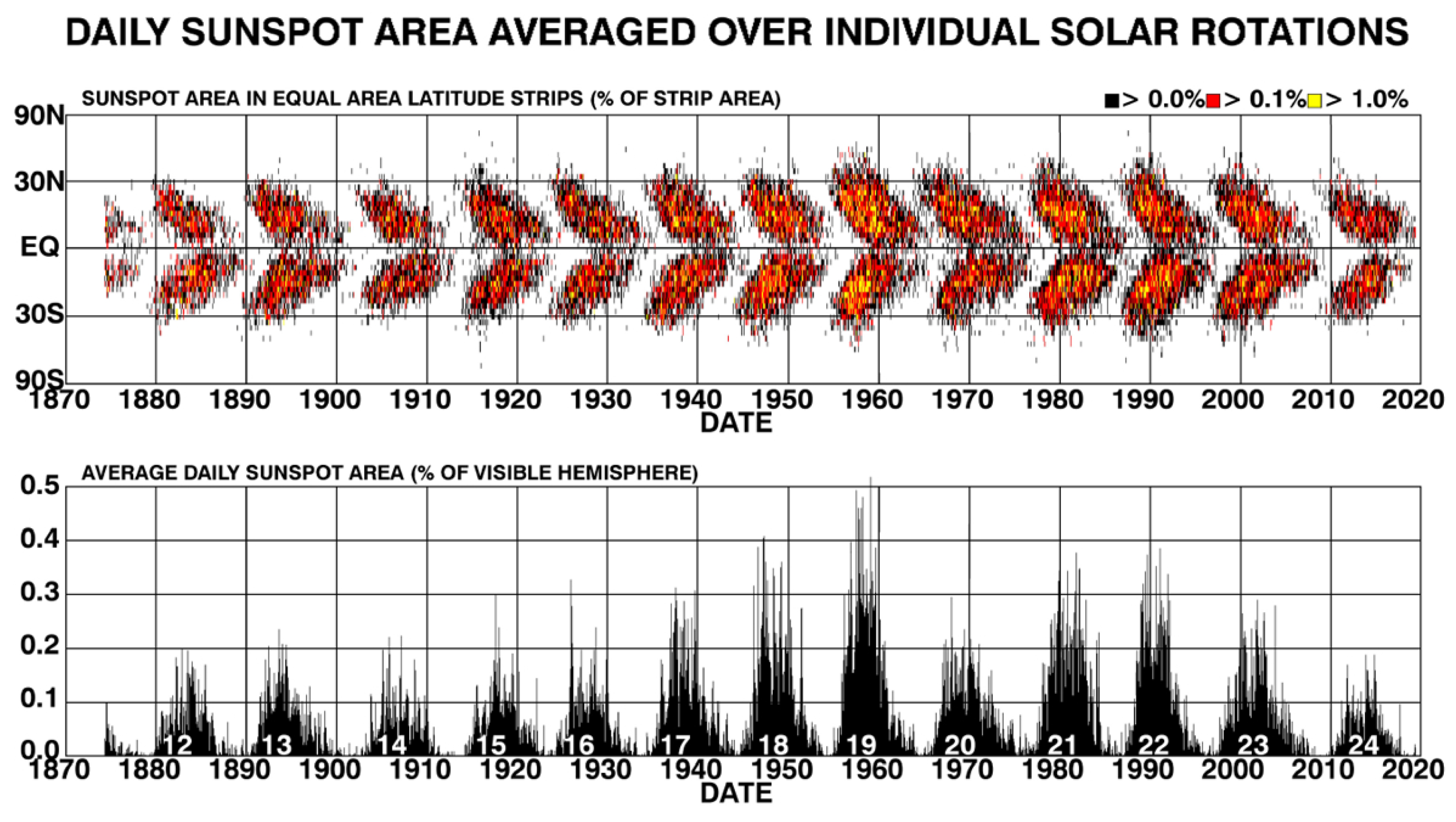
• The solar activity cycle is quasi-periodic. The periods range between 9 and 14 years, with a mean period of 11 years. Additionally, strong fluctuations have been observed in the cycle’s amplitude.
• Sunspots are observed to consist of pairs with opposite magnetic polarities [67]. It was observed that they are generally elongated in the East–West direction, with the leading polarities generally leaning closer to the Equator than the trailing polarities. Additionally, Hale noted that most leading spots have opposite polarities in opposite hemispheres. In addition, a reversal of polar magnetic fields near the time of cycle maximum has also been observed. This reversal is referred to as ‘Hale’s polarity Law’. As a consequence of this law, an underlying magnetic cycle of twice that period (approximately 22 years) is also present.
• Hale et al. [67] also showed that the sunspots observed on the solar surface show a systematic tilt, which increases with latitude, a phenomenon referred to as ‘Joy’s law’.
• The locations of sunspots show an equatorward drift of the active latitude, described by Spörer’s law [68].
• Long-term studies of the numbers of sunspots have revealed an 80-year cycle known as the Gleissberg cycle. This is in addition to 51.34, 8.83 and 3.77-year cycles [69,70]; the latter are manifested as hemispherical asymmetries.
• The Sun also exhibits a number of less dominant magnetic cycles [71].
• As we already saw in the Introduction, in addition to these reported observations of cyclic variations and sunspots, there has also been a period between 1645 and 1715 ([72], known as the ‘Maunder Minimum’); featuring an absence in solar activity, with very few sunspots observed.

The quasi-periodic nature of the solar cycle, in addition to the observational evidence which points to no apparent relation between the strengths of successive sunspot cycles, renders making predictions a challenging task [73]. The complex sunspot cycle can be expressed using a sunspot ‘butterfly diagram’ (see Figure 3), which shows the fractional coverage of sunspots as a function of solar latitude and time (for more details, see the reviews by [65,74] and references therein). In addition, assuming that the toroidal fluxes, which likely govern the appearance of sunspots, rise radially and are formed where the magnetic field is strongest, the sunspot butterfly diagram also reflects a spatio-temporal ‘map’ of the Sun’s internal, large-scale toroidal magnetic-field component.

2.2. The Solar Dynamo

Although it is well-known that solar activity is driven by the solar magnetic field and is produced by dynamo processes within the Sun, the details concerning how, when and where these dynamo processes operate are still uncertain. In this section, we outline the scientific background for modelling the solar cycle as a magnetohydrodynamic (MHD) process. We refer the reader to (Charbonneau [74] and references therein) for a detailed review of the solar dynamo. Relevant scientific background about the solar interior, the basic physics of the solar atmosphere and some elements of radiative transfer can be found in (Costas [75] and references therein).

2.2.1. Key Components of Dynamo Theory

Dynamo theory proposes that stars, including our Sun, possess physical mechanisms that generate a magnetic field. Figure 4 provides a schematic overview of the basic features of the solar dynamo. To fully understand solar (or stellar) dynamo theory we have to consider the key ingredients through which a convecting, rotating and electrically conducting fluid can maintain a magnetic field over cosmic timescales. These ingredients include the turbulent motions present in convective regions or, in some cases, also in radiative zones [76]. Additionally, it also includes processes that redistribute angular momentum to yield large-scale flows, such as differential rotation and meridional circulation, rotation-induced helicity and low diffusivity [77]. These nonlinear physical processes ultimately create, sustain and organise magnetic fields on all relevant scales. An in-depth review of the processes which generate magnetic fields is presented by Brun et al. [78]. Here we will briefly discuss how turbulent, rotating convection plays into dynamo theory.

Convection is an instability that occurs in a stratified fluid or plasma, which in turn leads to the transportation of energy through the bulk displacement of parcels of ‘fluid’. In stellar convection zones, convection carries most of the energy. To quantity the efficiency of convection we use the ‘Nusselt Number’, i.e., the ratio of convective to conductive heat transfer; the Nusselt Number ranges from zero to unity for pure convection to pure conduction. The Nusselt Number also quantifies the importance of convective transport relative to energy transport by other processes such as conduction or radiative diffusion.

The internal motion in stars is highly convective (turbulent). This can be quantified by the Reynolds number, $Re=uL/\nu$. Here, u represents the characteristic velocity, L is the characteristic length and $\nu$ the viscosity. Stars possess very high Reynolds numbers, which directly implies highly turbulent internal motions. However, no comprehensive theory exists as yet that can fully describe the complexity of turbulent, nonlinear, convective, rotating and magnetised systems. Nevertheless, to make up for the lack of a comprehensive theory for stellar convection zones, several approaches have been proposed and pursued. A commonly used theory to approximate convection and convective heat transport in stars is the Mixing Length Theory (MLT), first proposed by Böhm-Vitense [79]. We refer the reader to Brun et al. [80] (and references therein) for a review of the standard treatments of stellar or geophysical convection. We note that typical mixing-length prescriptions do not take explicit account of rotation or magnetism. However various efforts have been made to include the effects of rotation and magnetism (e.g., [81,82,83]).

Stellar rotation critically affects stellar dynamics (e.g., [84,85,86]) and plays a crucial role in stellar evolution. Rotation not only influences fluid flows, their turbulence and the transport of angular momentum within a given system, but it is also likely to trigger instabilities. Instabilities in moving plasmas is a field in itself. We refer the reader to the review by Maeder [87] for a detailed description of the main instabilities currently considered influential in the evolution of Sun-like stars. In brief, convective instabilities in stratified atmospheres in the inviscid limit ($\nu$ = $\kappa$ = 0, i.e., no viscous nor thermal dissipative effects) are well-constrained by the Ledoux criterion [88],

$$\Delta >{\Delta }_b+\frac{\varphi }{{\alpha }_t}{\Delta }_{{\mu }_M},$$

(1)

where ${\alpha }_t$ and $\varphi$ are the thermodynamic coefficients, ${\Delta }_{{\mu }_M}$ is the mean molecular weight, the subscript ‘m’ refers to the background medium and ‘b’ refers to a moving ‘blob’ (parcel) of fluid. The Ledoux criterion reduces to the Schwarzschild criterion (which describes a basic plasma that is stable against convection) when variations in composition or ionisation are neglected. The Schwarzschild criterion ($\Delta >{\Delta }_b$) in a stratified layer, where energy is solely transported by radiation (‘rad’) and the fluid element is displaced adiabatically (‘ad’), becomes ${\Delta }_{\mathrm{rad}}>{\Delta }_{\mathrm{ad}}$.

In a rotating star, the Ledoux or Schwarzschild criterion for convective instability should be replaced by the Solberg–Høiland criterion [89], which accounts for the difference in the centrifugal motion affecting an adiabatically displaced fluid element. In practice, convective stability is reinforced by rotation. In the absence of rotation, a zone located between loci where $\Delta ={\Delta }_{\mathrm{ad}}+{\Delta }_{\mu }$ and $\Delta$ = ${\Delta }_{\mathrm{ad}}$ is called ‘semiconvective’. In semiconvective zones, non-adiabatic effects can drive growing oscillatory instabilities [89,90]. Additionally, in radiative zones, differential rotation is likely a very efficient mixing process, and this drives shear instabilites [89,91]. Moreover, various other axisymmetric and non-axisymmetric instabilities may also occur. A detailed account of these additional instabilities is presented by Maeder [87].

Turbulent convection and rotation in stars therefore induce a rich array of interesting dynamical phenomena and directly play into dynamo theory. Dynamo activity in stars relies on the presence of an electrically conducting fluid (or plasma, or gas). It is the currents associated with motion in that fluid that ultimately drive the dynamo. The MHD induction equation (derived from Maxwell’s equations in the non-relativistic limit; see, e.g., [92]) explains how the induction or creation of magnetic fields is possible in principle,

$$\frac{\partial B}{\partial t}=\nabla \times (u\times B-\eta \nabla \times B),$$

(2)

where t represents the time, B is the magnetic field and $\eta$ is the magnetic diffusivity. Here, $\eta =c^2/4\pi {\sigma }_{\mathrm{e}}$, where ${\sigma }_{\mathrm{e}}$ is the electrical conductivity, which is in general only a function of depth for spherically symmetric solar/stellar structural models. A detailed derivation can be found in many textbooks and reviews (e.g., [93,94]).

The magnetic field must satisfy $\nabla ·B=0$. Additionally, the required evolution equation for the flow field, u, is described by the magnetic Navier–Stokes equations, augmented by the Lorentz force. This ensures conservation of momentum and takes the form of the force equation,

$$\frac{\partial u}{\partial t}+(u·\nabla )u=-\frac{1}{\rho }\nabla p+g+\frac{1}{4\pi \rho }(\nabla \times B)\times B-2\mathsf{\Omega }\times u+\frac{1}{\rho }\nabla ·\tau .$$

(3)

Here, $\tau$ represents the viscous stress tensor. All other symbols represent their standard meaning. MHD, i.e., the dynamics of magnetised fluids, is therefore defined by the combination of Equations (2) and (3), complemented by suitable equations expressing conservation of mass and energy, as well as an equation of state. The third term on the right-hand side (RHS) represents the Lorentz force. It explains why flux tubes exist. The Lorentz term can be expressed as the sum of a local negative pressure gradient, $B^2/8\pi$, and a tension term that maintains the integrity of the flux tubes.

The dynamo process is nonlinear. Therefore, it is critical to account for this nonlinearity. This can be done by considering the total magnetic energy within the system which is achieved by taking the scalar product of Equation (2) with B and integrating over volume V. This gives,

$$\frac{\mathrm{d}}{\mathrm{d}t}{\int }_V\frac{{\overrightarrow{B}}^2}{8\pi }\mathrm{d}V=-{\oint }_{\partial V}\overrightarrow{S}·\overrightarrow{n}\mathrm{d}A-\frac{1}{{\sigma }_{\mathrm{e}}}{\int }_V{\overrightarrow{J}}^2\mathrm{d}V-\frac{1}{c}{\int }_V\overrightarrow{u}·(\overrightarrow{J}\times \overrightarrow{B})\mathrm{d}V.$$

(4)

In Equation (4), S represents the Poynting flux (i.e, the directional energy). For isolated systems, such as for stars in a vacuum, the first RHS term can be neglected since its contribution is vanishingly small. The second term represents Ohmic dissipation of the electrical currents supporting the magnetic field. This will decrease magnetic energy everywhere except where ${\sigma }_{\mathrm{e}}$ tends to infinity. This is considered the ideal MHD limit. The third term on the RHS represents the dynamo contribution. An increase of magnetic energy can only occur if the flow does work against the Lorentz force. We note that here u represents the velocity of the flow, i.e., the displacement of a fluid element per unit time. Therefore, this conversion of mechanical energy into electromagnetic energy is the framework of any dynamo mechanism, including astrophysical dynamos.

Returning now to Equation (2), the first term on the RHS represents the inductive action of the flow field u. It acts as a source term for B and pertains to a characteristic timescale of the solar rotation period, approximately 27 days. The second term describes the resistive dissipation of the current systems supporting the magnetic field and is thus always a global sink for B. This latter term has a second derivative, which describes second-order effects such as the diffusion, evolution and disappearance of activity regions on timescales comparable to the full 22-year magnetic activity period. To first approximation, the magnetic Reynolds number ($Rm$) measures the relative importance of these two terms. The magnetic Reynolds number ($Rm$) can be obtained from dimensional analysis of Equation (2),

$$Rm=\frac{uL}{\eta }.$$

(5)

Here, $\eta$, u and L represent the standard values for, respectively, the magnetic diffusivity, flow speed and length scale over which B varies significantly.

The dynamo problem consists of finding or producing a (dynamically consistent) flow field u that has inductive properties capable of sustaining B against Ohmic dissipation. Ultimately, amplification of B occurs by shearing, compression and transport by the flow of the pre-existing magnetic field. This is readily seen upon rewriting the inductive term in Equation (2) as

$$\nabla \times \left(\overrightarrow{u\times B}\right)=(\overrightarrow{B}·\nabla )\overrightarrow{u}-\overrightarrow{B}(\nabla ·\overrightarrow{u})-(\overrightarrow{u}·\nabla )\overrightarrow{B}.$$

(6)

The terms on the RHS of Equation (6) correspond to the shearing, compression and transport of the pre-existing magnetic field by the flow. Shearing can lead to exponential amplification of the magnetic field, at a rate proportional to the local flow gradient.

When $u=0$, i.e., if there is no motion, the field must decay away on a characteristic timescale ${\tau }_{\eta }=L^2/\eta$. In the perfect conducting limit, i.e, the opposite limit of no diffusion, we have the ‘ideal MHD’ limit. Here, it can be shown that the magnetic flux through any closed loop (i.e., the surface integral of B over that loop) remains constant as the loop moves around, a result known as Alfvén’s theorem. In this regime, the magnetic field lines are fixed or frozen into the fluid. This means that they behave in accordance with the plasma, i.e., the magnetic field lines go where the plasma goes, the magnetic field lines are compressed (or diluted) where the plasma is compressed (or expands), respectively. Assessing field growth is as challenging as assessing the trajectories of particles in a given flow field. Thus, if the flow is sufficiently complex then we may expect the energy in the magnetic field to grow. More details on this topic can be found in Childress & Gilbert [95].

In the solar cycle context, we care about identifying the circumstances under which the flow fields observed and/or inferred in the Sun can sustain the cyclic regeneration of the magnetic field associated with the observed solar cycle. This is captured in the solar dynamo problem. In addition to sustaining a field, a model of the solar dynamo should also reproduce:

• the cyclic polarity reversals with a decadal half-period, equatorward migration of the sunspot-generating deep toroidal field and its inferred strength, poleward migration of the diffuse surface field, the observed $\pi$/2 phase lag between poloidal and toroidal components, polar field strength, observed antisymmetric equatorial parity and predominantly negative (positive) magnetic helicity in the Northern (Southern) solar hemisphere.
• the amplitude fluctuations, empirical patterns and correlations extracted from the sunspot and proxy records, including the Grand Minima, during which the cycle amplitude—and perhaps the cycle itself—is strongly suppressed over many cycle periods.
• the torsional oscillations in the convective envelope, with proper amplitude and phasing with respect to the magnetic cycle.

The solar dynamo problem is therefore very hard to tackle as a direct numerical simulation of the MHD equations. The challenges are many, including the disparity of time- and length scales involved, and the fact that the outer 30% (in solar radii) are the seat of vigorous, thermally driven turbulent convective fluid motions. Therefore, most solar dynamo modelling work has thus far relied on simplifications of the MHD equations, as well as on assumptions regarding the structure of the Sun’s magnetic field and internal flows. We refer the reader to the reviews by Charbonneau [33,74] for an in-depth overview of the type of drastic simplification of the MHD system usually employed; see also Mestel [96] for a more complete review of solar magnetism and the solar dynamo. Alternatively, one can attempt to simplify the problem’s geometry, e.g., by representing the prevailing magnetic field as being composed of purely poloidal and toroidal components. In the latter case and in the context of ideal MHD conditions, exact analytical solutions can, in fact, be obtained [97].

In brief, some simplifications include the kinematic approximation. In this case, Equation (3) is dropped by assuming a given u, thus making the MHD induction equation linear in B. This approximation works well since the solar convective envelope has a low amplitude of observed torsional oscillations. Additionally, the observed solar activity suggests that the large-scale solar magnetic field is axisymmetric about the Sun’s rotation axis and antisymmetric about its equatorial plane (to first approximation). In this case, ‘solar activity’ includes the sunspot butterfly diagram, the shape of the solar corona at and around solar activity minimum, synoptic magnetograms and Hale’s polarity law. As discussed in Section 2.1, Hale’s polarity law describes the tendency for bipolar active regions within the same hemisphere to have the same leading magnetic polarity. Those in the opposite hemisphere have the opposite leading polarity. This pattern reverses from one sunspot cycle to the next [67]. Also, given the prevailing circumstances, the large-scale field can be expressed as the sum of a toroidal (or longitudinal) component and a poloidal component (or contained in meridional planes).

The cyclic regeneration of the solar large-scale field can therefore be thought of as a temporal sequence comprising the poloidal (P) and toroidal (T) components. This takes the form

$$P(+)\to T(-)\to P(-)\to T(+)\to P(+)\to \dots$$

(7)

Here, (+) and (−) refer to the observationally established signs of the two components. A full magnetic cycle of period ≈ 22 years consists of two successive sunspot cycles, each of duration ≈ 11 years (see Section 2.1). The Sun’s poloidal magnetic component, as measured from photospheric magnetograms, peaks at the time of sunspot minimum. The Sun’s poloidal magnetic component reverses polarity near sunspot cycle maximum, which corresponds to the epoch of the peak internal toroidal field. Therefore, the dynamo problem can be divided into two subproblems, including (i) $P\to T$ and (ii) $T\to P$. The former refers to the generation of a toroidal field from a pre-existing poloidal component, and the latter refers to the generation of a poloidal field from a pre-existing toroidal component. We refer the reader to reviews by Brun et al. [80] and Charbonneau [74] for details about the two components. We also refer the reader to the study by Cameron et al. [98], who provide maps of the poloidal and toroidal magnetic fields pertaining to the global solar dynamo.

Currently, there is no universally accepted model, nor a predictive theory, for the operation of the global solar (or stellar) dynamo. In the following subsections, we briefly present two sets of dynamo models for the solar cycle discussed at length in the recent literature, the first based on mean-field theory and the second based on the Babcock–Leighton mechanism.

2.2.2. Mean-Field Models

Not all spatial scales of magnetism have equal influence on a star’s evolution. Therefore, in addition to the constraints on the overall level of magnetic energy, the magnetic field’s spatial structure and temporal variability are also important. By parameterising the total effects of the flows and fields, solar cycle models based on the mean-field dynamo theory proposed a solution for the evolution of these large-scale fields. The evolution equation for the large-scale field encompasses the statistical properties of the small-scale flow combined with bulk parameters like the rotation rate. Mean-field models are summarised in detail in the reviews by Brandenburg & Subramanian [99], Brun et al. [80] and Charbonneau [74], and numerous references therein.

2.2.3. Babcock–Leighton Flux Transport Models

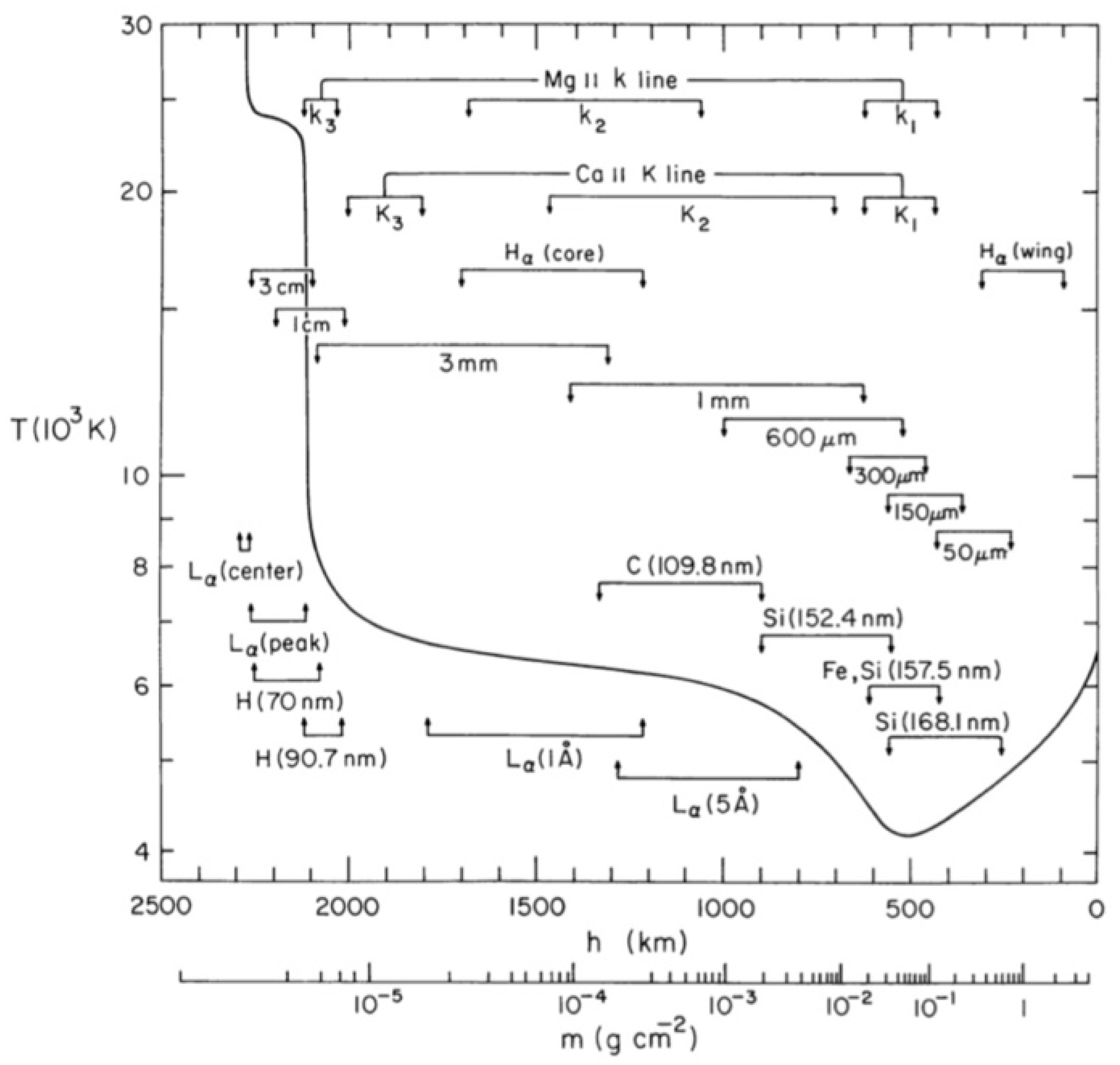
Several effects can generate a poloidal field from a toroidal field. The main physical mechanism behind the production of a poloidal field from a toroidal field, with rising convective eddies stretching the field and systematically twisting it, is helical convection. Additionally, as recognised by Babcock [32] and explored by Leighton [100,101], the poloidal field can also be generated by the decay of tilted active regions at the solar surface. Among others, Cameron & Schüssler [102] and Cameron et al. [98] have shown that the reversal of the surface poloidal field is triggered by this decay. Figure 5 provides a graphical overview of the Babcock–Leighton Flux Transport model.

Solar cycle models based on the Babcock–Leighton mechanism [32,100,101] remained overshadowed by mean-field electrodynamics until the late 1960s. The limitation of mean-field models and also observations of synoptic magnetographic monitoring over sunspot cycles 21 and 22 gave compelling evidence that the decay of active regions is mostly owing to the start of surface polar field reversals (e.g., [103,104], and references therein). This led to the revival of Babcock–Leighton models for the solar dynamo. These models are summarised more completely in the reviews by Charbonneau [33,74,105] and Brun et al. [80].

Figure 5. Overview of the main processes thought to occur during the solar cycle, departing from (a) an initial poloidal field. (b,c) Generation of the toroidal field through differential rotation. (d,e) Effect of cyclonic turbulence on former toroidal fields, creating small-scale secondary poloidal magnetic fields and resulting in a net electromotive force generating a new large-scale poloidal field (f), closing the first half part of the magnetic cycle with a new poloidal field (g), with opposite polarity compared with the initial field. (h) Beginning of the Babcock–Leighton mechanism: Toroidal flux tubes buoyantly rise to the surface, forming sunspots and tilted bipolar regions. (i) The fields from the bipolar regions diffuse and reconnect with each other and with the polar fields. The resulting poloidal flux is advected by meridional circulation to the poles, generating the final large-scale poloidal field in (g). (© Sanchez et al. [106]. Reproduced under a Creative Commons Attribution-NonCommercial 3.0 Unported License; https://creativecommons.org/licenses/by/3.0.

Figure 5. Overview of the main processes thought to occur during the solar cycle, departing from (a) an initial poloidal field. (b,c) Generation of the toroidal field through differential rotation. (d,e) Effect of cyclonic turbulence on former toroidal fields, creating small-scale secondary poloidal magnetic fields and resulting in a net electromotive force generating a new large-scale poloidal field (f), closing the first half part of the magnetic cycle with a new poloidal field (g), with opposite polarity compared with the initial field. (h) Beginning of the Babcock–Leighton mechanism: Toroidal flux tubes buoyantly rise to the surface, forming sunspots and tilted bipolar regions. (i) The fields from the bipolar regions diffuse and reconnect with each other and with the polar fields. The resulting poloidal flux is advected by meridional circulation to the poles, generating the final large-scale poloidal field in (g). (© Sanchez et al. [106]. Reproduced under a Creative Commons Attribution-NonCommercial 3.0 Unported License; https://creativecommons.org/licenses/by/3.0.

3. Diagnostics

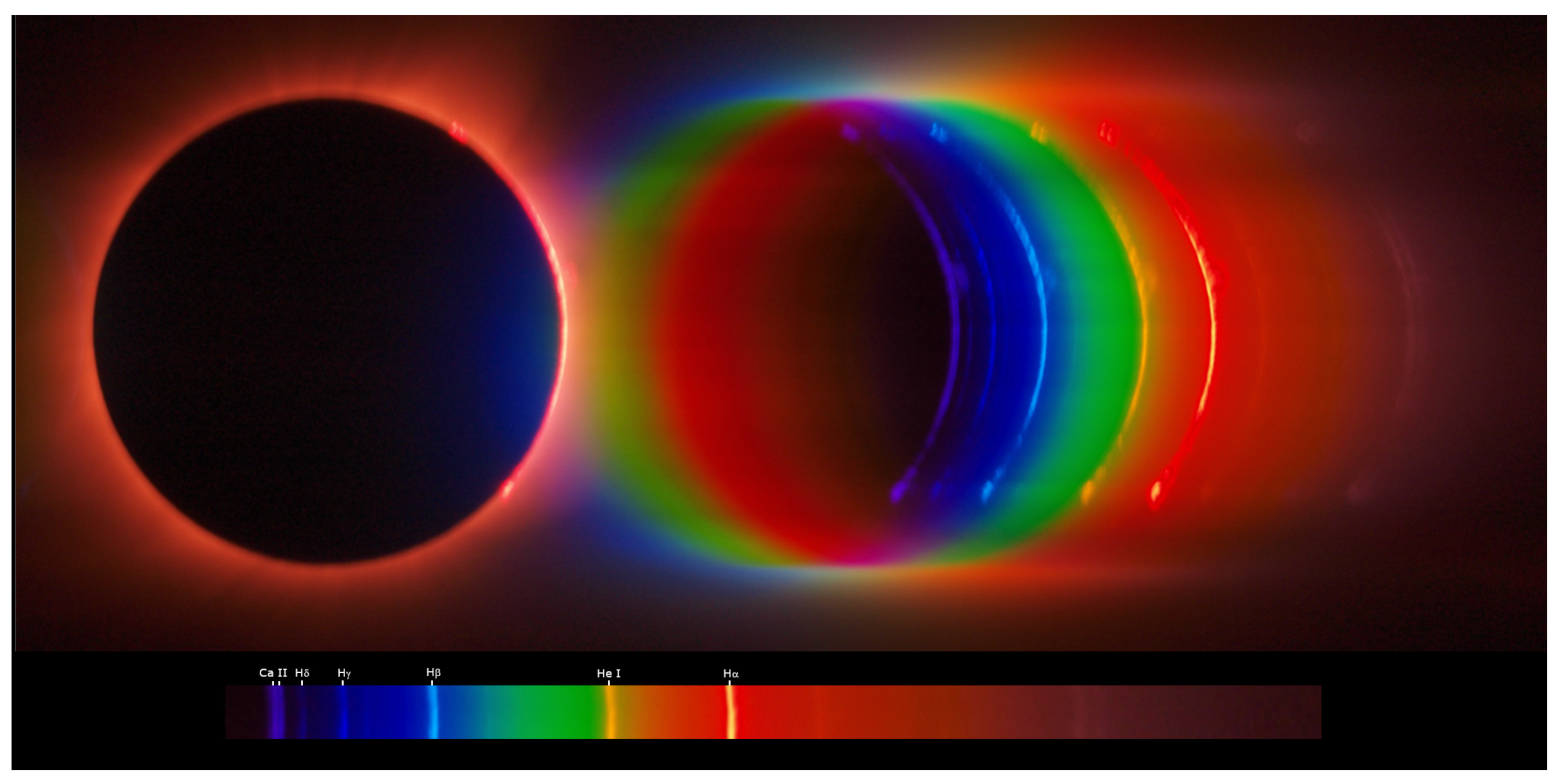
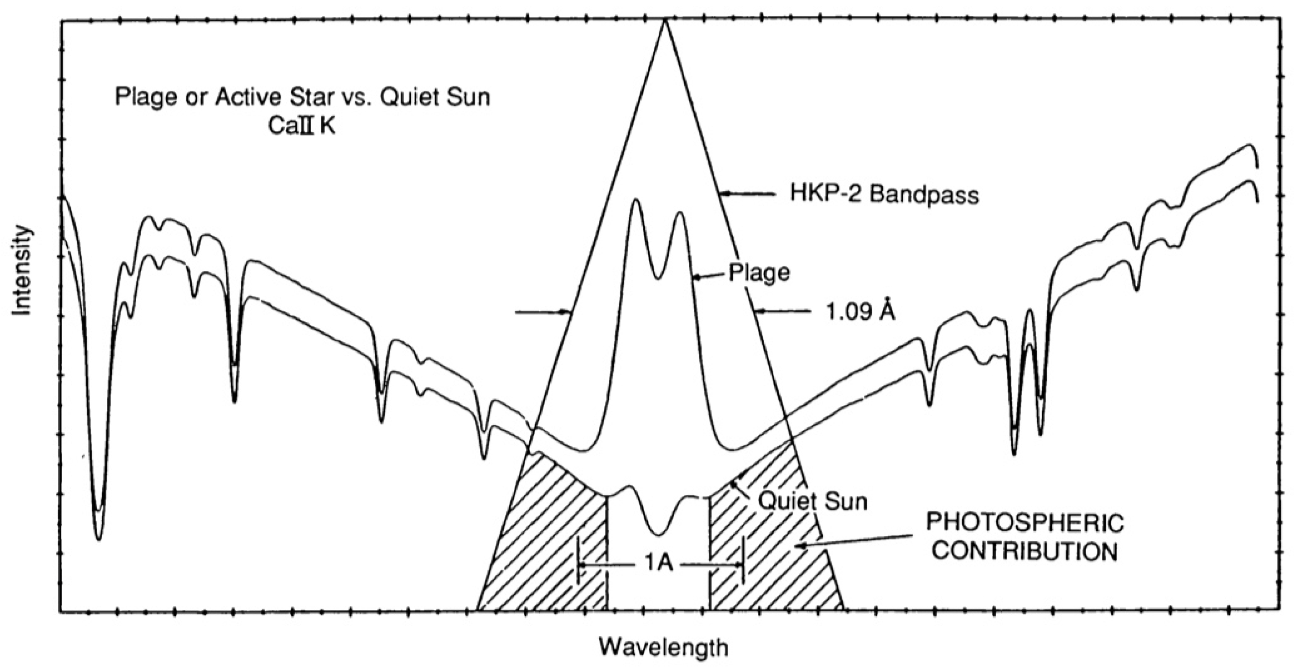
3.1. Spectroscopic Diagnostics

The first detection of stellar chromospheric line emission was achieved by Eberhard & Schwarzschild [107]. One of the most frequently used indicators of chromospheric activity in cool early-F to M-type stars is the occurrence of non-thermal flux reversal in the cores of the Ca ii H and K absorption lines centred at, respectively, 3968.470 Å and 3933.663 Å. Ca ii H and K ions originate in both the upper photosphere and the chromosphere; they are often associated with the presence of plages [108] and are sensitive to magnetic activity [109].

A range of other spectral activity indicators have also been explored and found useful as tracers of chromospheric magnetic activity (see Figure 6), flares and plages, including H$\alpha$ [4,110] and H$\beta$ emission [111], He i D${}_3$ (587.59 nm) and 1.08 $\mathsf{\mu }$m absorption [112,113,114,115], the Na i D${}_1$ and D${}_2$ lines, the infrared Ca ii triplet absorption lines (centred at 8498.062 Å, 8542.144 Å and 8662.170 Å), and extreme ultraviolet (UV; 200.5–300.5 nm) resonance lines associated with surface effective temperatures $T_{\mathrm{eff}}<2\times {10}^4$ K, including C i, C ii, Co ii, Cr ii, Fe ii, Mn ii, Ni ii, O i, Si ii and Ti ii [116], as well as Mg ii h and k [117,118,119]. Of these, Fe ii (298.5 nm) is the dominant contributor to solar irradiance variations in high-ionisation environments [114].

Note that H$\alpha$ shows up as an emission line in magnetically active stars (see, e.g., Figure 7), whereas it manifests itself as filled-in absorption in less active stars. This is so, because with increased heating rates, H$\alpha$ absorption initially becomes deeper before it turns into an emission-line profile [120]. The He i 1.08 $\mathsf{\mu }$m absorption line is observed in many G- and K-type stars, and particularly in binary systems (see Section 5). Its presence is somewhat puzzling, however. In ordinary late-type stellar atmospheres, this line should not exist, given that the metastable lower state of the transition that produces it is located just 20 eV above the ground state. It is therefore thought to be produced at high altitudes and at high temperatures, e.g., in a star’s chromosphere or corona [121].

The Ca ii infrared triplet lines are of particular interest given that they offer a number of distinct advantages with respect to the workhorse Ca ii H and K lines. The ratio of the equivalent widths (EWs) of the Ca ii triplet lines at 8542 Å and 8498 Å, EW${}_{8542}$/EW${}_{8498}$, is an indicator of chromospheric activity that is particularly suitable to distinguish between the occurrence of plages and prominences [113]. Zhang et al. [113] recorded these line ratios for the chromospherically active, late-type spectroscopic RS CVn binary system DM UMa. They found EW${}_{8542}$/EW${}_{8498}$ ratios of 1.0–1.7, which implies the presence of optically thick plages. This is typical of many late-type stars [111,122,123,124,125,126].

The infrared triplet lines are formed in the lower chromosphere through subordinate transitions between the excited levels of Ca ii $4^2$ P${}_{1/2,2/3}$ and meta-stable $3^2$ D${}_{3/2,5/2}$ [127,128]. The result of this is increased atmospheric activity and strong lines. In turn, this allows us to gain insights into the physical conditions throughout a significant depth range in the stellar atmosphere [41,127]. These lines are mostly collisionally controlled. Hence, they are highly sensitive to the ambient temperature [129] and, thus, they are key tracers of chromospheric activity [41,128,130,131,132].

From a practical perspective, the Ca ii triplet lines are found in a spectral region that is less subject to telluric contamination than the UV regime covering the Ca ii H and K lines [132,133]. The longer-wavelength range of the infrared triplet is also less affected by photospheric lines, thus facilitating more straightforward spectral processing and calibration. Moreover, the Ca ii infrared triplet lines are less sensitive to rapid variability caused by flares and other transient emission features, hence allowing for more robust measurements of the mean level of stellar chromospheric activity. This is of particular importance for the later, K- and M-type, stars, which have blackbody characteristics that peak at longer wavelengths.

From a physical perspective, the Ca ii triplet line profiles and their wings are sensitive to fundamental stellar parameter variations, including in the effective temperature, metallicity and surface gravity [134]. This thus offers insights into galactic chemical enrichment histories through measurements of Ca abundances and $\alpha$ enrichment in late-type dwarfs [135]. Note, however, that higher-quality spectra are required for Ca ii infrared triplet analysis than for H$\alpha$ or Ca ii H and K line analysis.

The shape of the Mg ii h and k lines is the result of a combination of photospheric and chromospheric processes. The line cores are generated in the chromosphere, whereas the wings reflect conditions in the upper photosphere [119]. The relationship between the stellar surface area covered by plages and the irradiance variations traced by the Ca ii K, Mg ii h and k, and He i lines has been the subject of numerous studies [114,136,137,138].

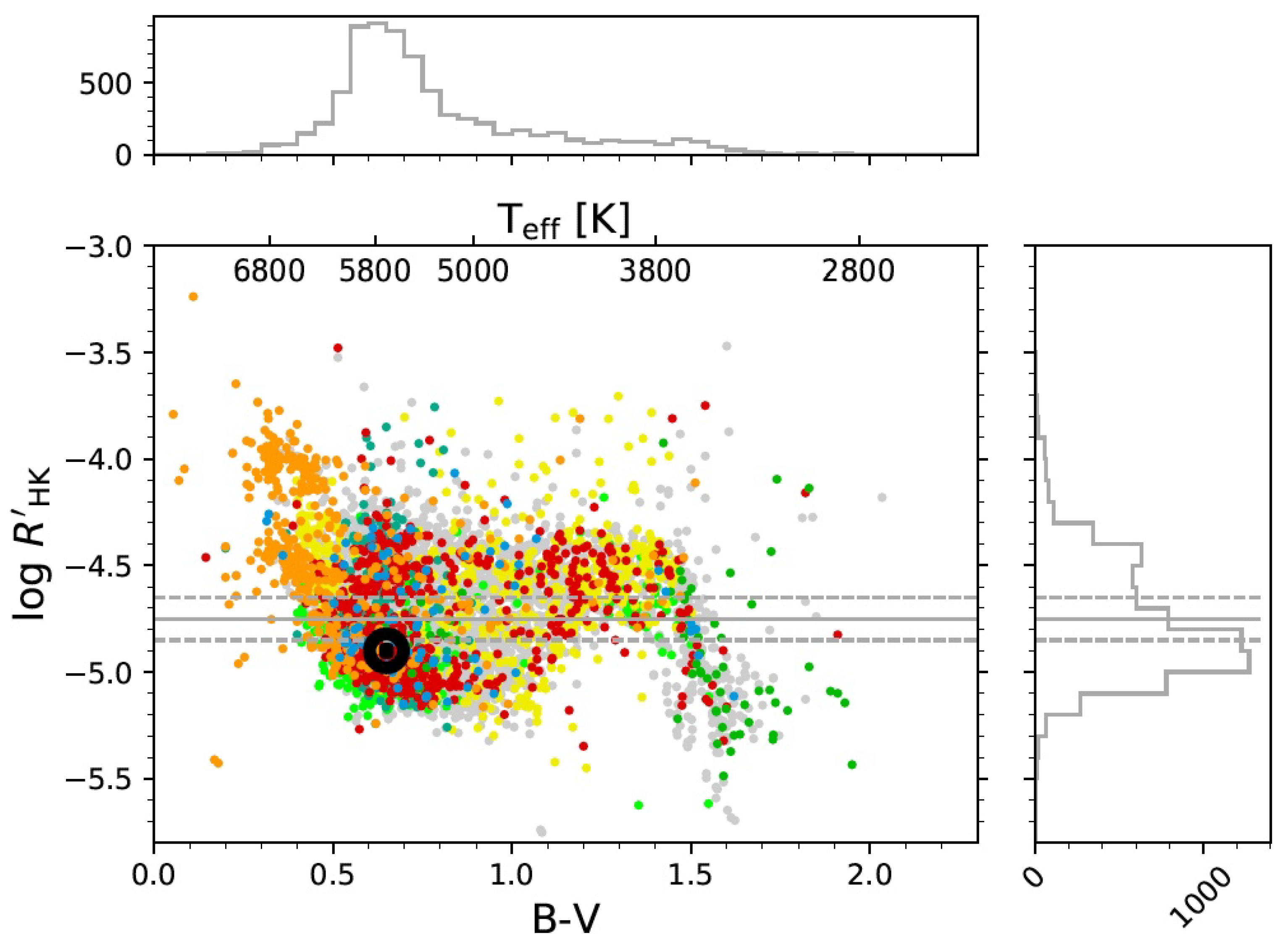
3.2. The Mt Wilson S Index

Although analyses of carefully selected spectral-line characteristics are preferred to obtain the highest-quality physical parameters of chromospherically active stars, integrated quantities such as bolometric flux-normalised indices [134,139], EWs [132,140] and absolute chromospheric fluxes are often employed instead. For instance, Schrijver & Zwaan [141] provide a power-law parameterisation of the relationship between the magnetic flux density, $|{\varphi }_i|$, and the corresponding radiative diagnostic (i.e., the relevant flux measure), $F_i$,

$$F_i=a_i{\left|{\varphi }_i\right|}^{b_i},$$

(8)

where $a_i$ is a proportionality constant, i refers to the relevant diagnostic—e.g., X-ray flux [142], Ca ii H and K core emission—and the exponent $b_i$ increases monotonically with increasing temperature; it ranges from $b_i$∼0.5 for Ca ii and Mg ii chromospheric emission to approximately 0.75 for emission from the transition region (e.g., Si iv, C iv), to close to unity for coronal X-ray emission [141,143].

However, the physical interpretation of integrated quantities is not straightforward, given that these measures are not true reflections of chromospheric radiative losses [128]. Nevertheless, the Mt Wilson chromospheric activity index, $S_{\mathrm{MW}}$ (Equation (9)), is the most commonly employed chromospheric activity diagnostic [144,145,146,147]. For some stars, including the Sun, empirical S indices have been measured since the 1960s, primarily through monitoring at Mt Wilson, Lick and Lowell Observatories. It is derived by measuring the chromospheric Ca ii H and K line fluxes, normalised to the nearby continuum:

$$S_{\mathrm{MW}}=\alpha \frac{H+K}{R+V},$$

(9)

where H and K are the line fluxes measured in 1.09 Å-wide triangular bandpasses (full width at half maximum, although sometimes 2 Å windows are used; see Figure 8), whereas R and V represent estimates of the ‘pseudo-continuum’ on either side of the lines, measured in 20 Å-wide spectral windows centred on 3901.07 Å and 4001.07 Å; $\alpha$ is a normalisation constant, used to link any sample of stars to the Mt Wilson and Lowell Observatories’ reference sample [145,148,149].

The $S_{\mathrm{MW}}$ index requires a correction for line blanketing, i.e., the contribution from photospheric flux in the line cores. We also need to account for (i.e., normalise) the star’s bolometric luminosity. The index resulting from having applied the latter corrections is known as $R_{\mathrm{HK}}^{\prime }$ [139,148]. As a first step, we need to convert $S_{\mathrm{MW}}$ to $R_{\mathrm{HK}}$, the total flux in units of erg cm${}^{-2}$ s${}^{-1}$ at the stellar surface in the Ca ii H and K lines, normalised by the bolometric flux, i.e., [128,150]

$$R_{\mathrm{HK}}=\frac{F_{\mathrm{HK}}}{\sigma T_{\mathrm{eff}}^4},$$

(10)

where $\sigma$ is the Stefan–Boltzmann constant. Wright [147] calibrated $R_{\mathrm{HK}}$ as a function of $(B-V)$ colour for late-F to M-type stars [151,152]:

$$R_{\mathrm{HK}}=1.34\times {10}^{-4}{C}_{\mathrm{cf}}{S}_{\mathrm{MW}},$$

(11)

where

$$log{C}_{\mathrm{cf}}(B-V)=1.13{(B-V)}^3-3.91{(B-V)}^2+2.84(B-V)-0.47.$$

(12)

We next need to account for photospheric contamination of the line profiles, i.e.,

$$log{R}_{\mathrm{phot}}(B-V)=-4.898+1.918{(B-V)}^2-2.893{(B-V)}^3,$$

(13)

so that

$$R_{\mathrm{HK}}^{\prime }=R_{\mathrm{HK}}-R_{\mathrm{phot}}.$$

(14)

The photospheric contribution, $R_{\mathrm{phot}}=F_{\mathrm{phot}}/\sigma T_{\mathrm{eff}}^4$, is most often derived using the approach of Noyes et al. [139], which is based on the Hartmann et al. [153] method. It is, however, only valid for stars with $0.44\le (B-V)\le 0.82$ mag. Boro Saikia et al. [70] extended the colour baseline to include stars as red as $(B-V)=2.0$ mag.

This approach relies on some level of overlap between one’s target sample and the Mt Wilson and Lowell Observatories’ reference sample (or other, more recently established reference samples) [22]. In the absence of any meaningful overlap, one can rely on measurements of the excess flux, $\Delta F_{\mathrm{Ca}}$, instead [42]. The latter quantity is defined as the stellar surface flux triggered by magnetic activity. It can be calculated by subtracting the photospheric flux and the ‘basal’ flux from the flux in the Ca ii H and K lines [154]:

$$F_{1\mathrm{A}}={10}^{-14}{S}_{\mathrm{MW}}{C}_{\mathrm{cf}}{T}_{\mathrm{eff}}^4,$$

(15)

where [155]

$$log{C}_{\mathrm{cf}}=0.25{(B-V)}^3-1.33{(B-V)}^2+0.43(B-V)+0.24.$$

(16)

Karoff et al. [42] provided a calibrated relationship between $R_{\mathrm{HK}}$ and the Middelkoop [155] or the updated Rutten [154] conversion factor, $C_{\mathrm{cf}}$:

$$R_{\mathrm{HK}}=1.34\times {10}^{-4}{C}_{\mathrm{cf}}{S}_{\mathrm{MW}}.$$

(17)

The ‘basal’ flux used here is equivalent to the low chromospheric activity boundary [154,156,157,158,159]. For magnetically inactive stars, this pertains to their entire surface [160,161]. This basal (in)activity—referred to as ‘immaculate photospheres’ by Livingston et al. [162]—may be owing to acoustic heating [161,163], turbulent dynamo activity from non-rotating plasma [164] or low-frequency MHD wave heating through leakage into the lower chromosphere via inclined magnetic flux tubes [163,165]. The basal activity is almost constant for stars with $(B-V)\le 1.1$ mag; for stars with $1.1\le (B-V)\le 1.4$ mag, the basal flux increases linearly with increasing $(B-V)$ colour [70]. Although this trend could imply a faster spin-down rate for cooler and older stars [139], such rapid changes in the spin-down rates of cool stars are not expected (see below; [166]). At even redder colours, chromospheric activity becomes weaker [167,168].

The calibration of $R_{\mathrm{HK}}^{\prime }$ depends on metallicity and evolutionary state, and hence on stellar colour, in the sense that higher metallicities lead to suppression of the measured $R_{\mathrm{HK}}^{\prime }$ values [169,170,171]. For dwarfs, a lower boundary to $R_{\mathrm{HK}}^{\prime }$ has been determined; it is a function of metallicity, [M/H] [171]:

$$R_{\mathrm{HK}}^{\prime }=-0.213[\mathrm{M}/\mathrm{H}]-5.125.$$

(18)

Fundamentally, this metallicity/evolutionary-state dependence renders a direct comparison of $S_{\mathrm{MW}}$ for different spectral types unsuitable: for later spectral types, stars become redder, and so typical K or M dwarfs will naturally have significantly larger $S_{\mathrm{MW}}$ indices. This will also have important ramifications for interpretations of the chromospheric activity–age relation, which we will discuss below. Direct comparisons of $R_{\mathrm{HK}}^{\prime }$ are less affected, since the latter index is a straight measure of the ratio of the chromospheric to the bolometric flux.

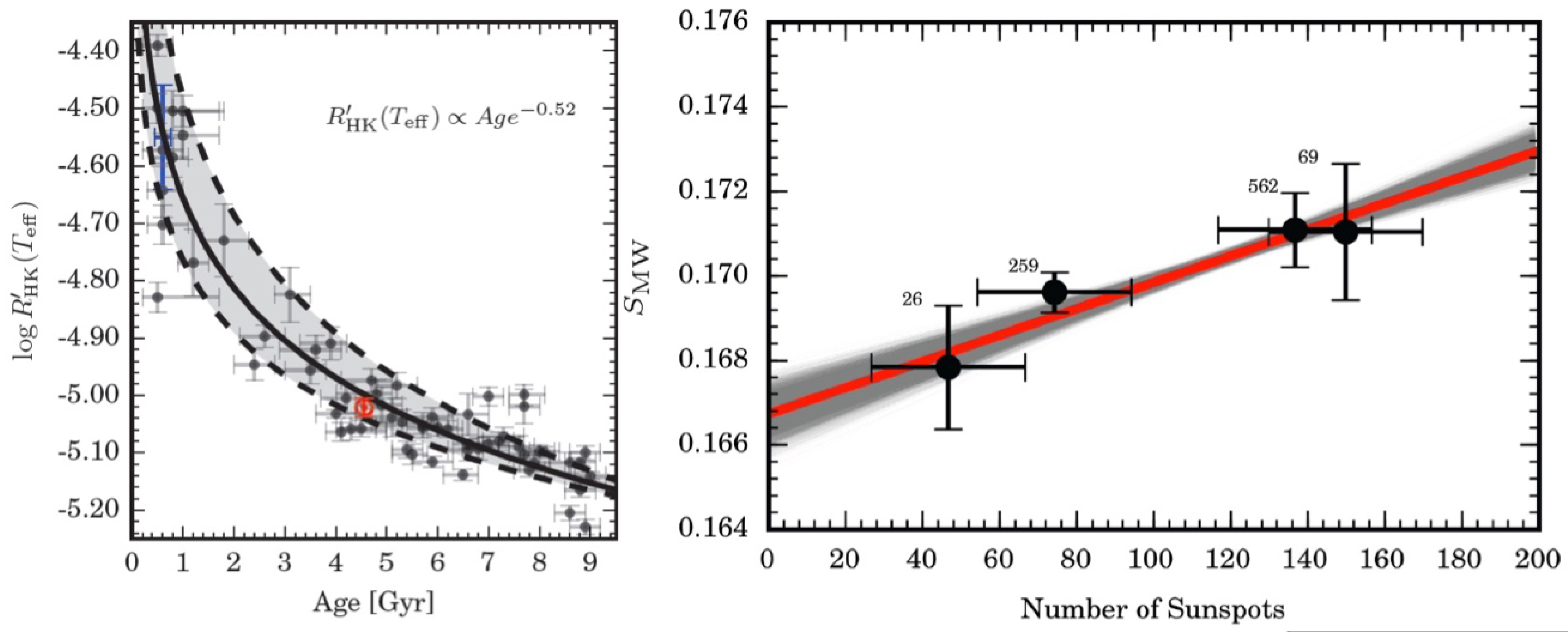
3.3. The Chromospheric Activity–Age Relation

Perhaps the most important diagnostic relationship allowing us to probe the physics of stars exhibiting chromospheric activity is the chromospheric activity–age relation. It was first established by Skumanich [34] in the early 1970s on the basis of Ca ii H and K emission, diagnostic lines that were straightforward to observe from most ground-based observatories at the time. Until recently, it was thought that chromospheric activity declines smoothly, rapidly and monotonically with increasing age [35,39] for ages up to about 1.5 Gyr [38,40], beyond which any activity would cease.

The physical mechanism thought responsible for this behaviour is the notion that stars lose mass through coronal winds, which in turn leads to a reduction in angular momentum as well as in the torque acting on the stellar surface. In combination, these effects lead to a gradual decrease in the stellar rotation rate on million-year timescales. Thus, the extent of braking owing to the decreasing stellar rotation is directly related to a reduced efficiency in the generation and amplification of magnetic fields at the base of the convection zone [25,41]. Consequently, a reduction in chromospheric heating follows [139]. Observationally, this will lead to a decrease in the chromospheric flux in the cores of the diagnostic absorption lines as a function of increasing stellar age.

However, in a series of recent papers Lorenzo-Oliveira et al. [26,41] have challenged this paradigm. They showed, based on observations of G dwarfs in old open clusters as well as a sample of 82 solar twins, that the smooth, monotonic decrease in activity extended with high significance (characterised by a false-alarm probability of just 1%) to ages of at least $t=6$–7 Gyr for solar-mass, solar-metallicity stars aged 0.6–9 Gyr [34,35,39,58,172] (see Figure 9, left):

$$\langle R_{\mathrm{HK}}^{\prime }\rangle \propto t^{-0.52}.$$

(19)

Lorenzo-Oliveira et al. [26,41] suggested that the earlier conclusion of activity cessation at ages of ∼1.5 Gyr might have been caused by a dependence of the Ca ii H and K fluxes on mass, effective temperature and metallicity, in addition to selection biases owing to stellar binarity or multiplicity and contamination by interstellar absorption lines [173] (see also [38]). Stellar multiplicity can alter the angular momentum evolution of the primary star [174,175], allowing it to maintain its rotation rate and magnetic activity to old age. Lorenzo-Oliveira et al. [41] found that the infrared Ca ii triplet lines are particularly sensitive to chromospheric activity in FGK-type stars, thus allowing exploration of the chromospheric activity–age relation for a wide range of magnetic activity levels, effective temperatures, stellar masses, metallicities and ages.

3.4. Correlations with Starspot Number

Bertello et al. [176] showed that the solar integrated Ca ii index correlates linearly with photospheric sunspot number, whereas the Ca ii line fluxes correlate better with solar chromospheric plages (see also [49]). Both phenomena are associated with magnetic activity. The latitude dependencies of plages and sunspots are similar, whereas the largest solar plages are typically associated spatially with dark sunspots [163,177,178,179]. Lorenzo-Oliveira et al. [26] established a robust and reproducible mean relationship between solar chromospheric activity and the international sunspot number,1 N (see Figure 9, right):

$$S_{\mathrm{MW}}=(3.12\pm 0.28)\times {10}^{-5}N+(0.1667\pm 0.0003).$$

(20)

Nevertheless, it is as yet unclear whether the correspondence between chromospheric activity and starspot number is sufficiently tight to warrant the derivation of long-term chromospheric activity cycles similar to those of the well-known photometric cycles [7,180,181].

The Sun is known to exhibit strong correlations among its chromospheric activity, photospheric flux and eigenmode frequencies (i.e., the normal frequencies with which the entire system oscillates in a sinusoidal manner; e.g., [22]). Changes in these parameters are all driven by magnetic flux tubes in the solar interior, which are responsible for changes in the turbulent velocities in the surface convection zone, thus affecting the eigenmode frequencies [182,183]. In turn, these changes lead to dark sunspots and bright faculae in the photosphere, whereas plages are formed in the chromosphere [55]. Karoff et al. [42] found that stars that are more chromospherically active than the Sun tend to evolve from starspot-dominated to faculae-dominated; magnetically inactive stars exhibit more constant spot-to-faculae ratios. The change in the relative dominance of starspots in active stars may be related to shifts in the distribution of a star’s active regions, in the sense that the area covered by starspots increases whereas the plage-dominant area becomes more spatially homogeneous [42,184].

Similar correlations between photospheric starspots and chromospheric plages have been found for other stars [185,186,187,188,189], although we clearly do not have access to the same physical scales for other stars as for the Sun. However, Morris et al. [190] showed that this limitation can be overcome by a combination of time-resolved spectroscopy and precision photometry. Plages can be traced through observations of the cores of the Ca ii H and K lines, whereas stellar fluxes are reduced when a significant fraction of the near-side surface of a star is covered by dark starspots ([190], and references therein).

Correlations between starspot and plage behaviour often manifest themselves as a dependence of the chromospheric variability on orbital phase or longitude [113,190]. This type of chromospheric variability reflects a star’s rotational modulation. In turn, this can be used to compute the minimum spot covering fraction via the so-called ‘flux deficit’ [190] (see also [179]),

$$f_{\mathrm{S},\min }=\frac{1-\min F}{1-c},$$

(21)

where F is the stellar flux and c is the spot contrast; $c=0$ represents a spot that is indistinguishable from the stellar photosphere, whereas $c=1$ is a completely black spot (for the Sun, $c=0.3$; [191]). As a star rotates and its spots and associated plages rotate into view, one would expect the $S_{\mathrm{MW}}$ index to increase and the continuum flux to decrease simultaneously. However, for a number of their sample G and K stars, Morris et al. [190] pointed out that as the dark spots rotate out of view, we continue to see evidence of chromospheric emission (see also [179]). This suggests that the network of plages on those stars is more extensive than the distribution of the dark starspots. As such, the putative correlation between chromospheric emission and starspot number remains poorly constrained.

3.5. The Vaughan–Preston Gap: Dependence on Stellar Rotation

The Mt Wilson survey of stellar chromospheric emission [144,145,146], which monitored more than one thousand stars over more than four decades until 2003, separated stars into magnetically active and inactive targets [192,193,194,195]. The apparent lack of stars exhibiting intermediate activity has become known as the Vaughan–Preston gap [196]. The original authors suggested that the perceived gap among a sample of 486 F- and G-type stars from the Mt Wilson survey might be caused by small-number statistics (selection effects) rather than by a true dearth of intermediate-activity stars [139]. Nevertheless, their study triggered a significant increase in theoretical follow-up studies attempting to explain the physical reality of the Vaughan–Preston gap. It is noteworthy that the Vaughan–Preston gap seems confined to F- and G-type stars, whereas it is not seen among cooler dwarfs [3].

Theoretical explanations put forward to reconcile the Vaughan–Preston gap can be classified as either an indication of two distinct stellar properties or due to some kind of temporal effect [139,196]. Among the former are suggestions of two distinct stellar populations [146,196,197], with young and active stars exhibiting higher values than their old and inactive counterparts, different stellar dynamo modes or topologies [155,196,198,199] or rapid, mass-dependent changes in differential rotation, possibly combined with a critical rotation rate [3,139,200]. Alternatively, a number of authors have suggested that the Vaughan–Preston gap may be caused by a smooth [139], rapid [201] or critical spin-down rate of the stellar rotation [139,155,196].

Saar & Brandenburg [194] reported the presence of multiple magnetic cycles in the Mt Wilson sample of cool stars, where stars initially found on the active (inactive) branch could exhibit a second cycle on the inactive (active) branch. This implies that a simple separation of stellar magnetic activity into clearly distinct active and inactive branches may not be appropriate. Similarly, Böhm-Vitense [199] (see also [146,194,200,202]) also found evidence of the presence of multiple cycles and the rapid migration of stars between the active and inactive branches, presumably on timescales of ∼200 Myr [201]. Multiple cycles are most likely detectable in rapidly rotating stars [202]; magnetic cycles can be both regular, i.e., solar-like, and irregular [70,146].

Scrutiny of the Mt Wilson sample of F–M-type dwarf stars revealed four types of stellar chromospheric activity cycles, including variable (25%), (apparently) cyclic (60%), trend and flat activity (15%) [146]. The more evolved Mt Wilson sample was roughly evenly split between variable (40%) and cyclic activity (40%, of which 20% exhibited well-defined cycles) [203], thus implying that as stars evolve their regular activity tends to become more chaotic. The remainder showed flat activity.

On the whole, cycle lengths correlate with rotation period, in the sense that longer rotation periods tend to produce longer cycles, with a clear distinction between active and inactive branches [199,204,205]. Stars exhibiting cyclic behaviour are characterised by dynamo periods $P_{\mathrm{cyc}}$ between 2.5 and 25 years, which shows some relatively poorly defined level of correlation with either the star’s rotation period or its Rossby number, i.e., the ratio of the stellar rotation period and the correlation timescale of the turbulence. Gomes da Silva et al. [206] expanded the sample of available M dwarfs, but although half of their 27 M0–M5.5 dwarfs showed significant cyclic behaviour, a correlation between cycle length and rotation period could not be determined [207]. By contrast, the activity–rotation relationship is very clear, in the sense that the stellar chromospheric emission $\langle R_{\mathrm{HK}}\rangle$ is inversely proportional to the Rossby number over a wide range of spectral types down to early-M stars [208], except for very fast rotation rates [209].

Photometrically, active stars tend to show more chaotic cyclic behaviour—including flip-flop behaviour involving flips between two permanent active longitudes every few years [210,211,212] and smaller phase jumps [213,214,215]—than their ‘normal’ counterparts [205,216]. Nevertheless, Messina & Guinan [217] found that the observed cycle lengths seem to converge with stellar age towards the solar cycle value at the Sun’s age, whereas the overall short- and long-term photometric variability increases with inverse Rossby number.

The Sun appears to be an anomaly for a star of its colour (temperature) and rotation period, since it does not coincide with either the active or inactive branches [200]. It is found somewhat closer to the low chromospheric activity boundary. Recently, Boro Saikia et al. [70] showed that the perceived bimodality in chromospheric activity may indeed have been a size-of-sample effect rather than a physical distinction between stars exhibiting either high or low magnetic activity. They found a higher fraction of activity among bluer and hotter stars, $(B-V)<0.5$ mag, compared with their redder counterparts, $(B-V)>0.5$ mag: see Figure 10. Moving from cooler to hotter temperatures, stars are characterised by rapidly increasing rotational velocities (for a classical reference, see [218], his Table 1). In turn, this may lead to the Ca ii H and K line wings becoming filled in, thus resembling chromospheric activity [219]. To date, the available evidence suggests that stars may spin down from high to low magnetic activity, although rapid spin-downs at intermediate activity have not been observed. A robust assessment as to whether or not this suggestion is borne out by reality requires accurate determinations of stellar ages and robust measurements of stellar rotation. The alternative scenario, where the Vaughan–Preston gap is the natural result of the presence of two or more dynamo mechanisms or geometry can be tested through a combination of up-to-date dynamo models and spectrophotometry [70]. Nevertheless, theoretical approaches using MHD simulations of global convective dynamo modes for a wide range of rotation rates have thus far only offered support for the reality of inactive branches [220,221].

4. Chromospheric Activity across the Hertzsprung–Russell Diagram

4.1. Solar-Type FGK Stars

The Mt Wilson survey confirmed that cool FGK-type main-sequence stars other than the Sun also routinely exhibit magnetic activity cycles [146]. However, unlike the long-term solar cycle, cool stellar magnetic activity can be categorised into three distinct types, including solar-like cyclic activity, highly variable non-cyclic activity and flat activity [70]. Marsden et al. [222] concluded, based on the high-resolution spectropolarimetric BCool survey, that surface magnetic fields associated with chromospheric activity can be detected for stars with $S_{\mathrm{MW}}$ indices in excess of ∼0.2.

F-type stars are characterised by very thin outer convection zones. As a consequence, they exhibit irregular variability rather than proper stellar cycles [223,224,225,226]. This may imply that the physical mechanism at the basis of this type of stellar variability differs from that driving longer-term stellar cycles [45,46].

G- and K-type stars, including the Sun, tend to exhibit secondary, shorter-term cycles [146,202,227,228,229,230], which may be manifestations of a second stellar dynamo in addition to that responsible for the main stellar (and solar) cycles. It has been suggested that such secondary dynamos might be evidence of polarity-reversing solar(-like) activity cycles [231]. This could be confirmed using Zeeman–Doppler imaging.

4.2. Late-Type Giant and Supergiant Stars

Chromospheric and coronal activity in evolved late-type stars has been studied for a long time (e.g., [232,233]) but remain poorly understood. Studies, especially in the X-ray and UV regimes, (e.g., [56,234,235,236]) have been carried out to investigate the evolution of coronal activity of late-type stars as a function of age. The more recent of these studies have also investigated the impact of chromospheric activity on the evolution of planetary atmospheres. By and large, some subsets of evolved late-type stars show a range of chromospheric and coronal activity but, in general, chromospheric activity and rotational rates decline with age.

Rutten [3] and Strassmeier et al. [237] showed that giant stars exhibit a general decrease in their Ca ii fluxes as a function of increasing rotation period, $P_{\mathrm{rot}}$, although with a large scatter about the mean. Whereas for a given $(B-V)$ colour the masses of main-sequence stars are well-constrained, giants span a range of stellar masses. As such, one would not expect a strong and unique correlation between $P_{\mathrm{rot}}$ and $R_{\mathrm{HK}}^{\prime }$, given that the structure of the convection zone will depend on the star’s mass and evolutionary state. Jordan [238] has shown, using the sample of Rutten [3], that $R_{\mathrm{HK}}^{\prime }$ for giants appears to ‘saturate’ at $log{R}_{\mathrm{HK}}^{\prime }$∼$-4.5$ at short periods, although at lower values than for main-sequence stars.

As discussed in Section 2.2, in young stars convection, rotation and turbulent motion drive a magnetic field which powers their dynamo action and results in significant magnetic chromospheric activity. During the evolved phases, such as the giant phases, stars undergo radial expansion and mass loss, which result in the decay of stellar rotation. Whether the chromospheric activity in evolved stars is due to either the presence of magnetic fields or the dissipation of mechanical waves, or a combination of both, remains poorly understood.

Observations of cool, evolved giants, supergiants and asymptotic giant-branch (AGB) stars with the International Ultraviolet Explorer (IUE), the Hubble Space Telescope (HST), and the GAlaxy Evolution EXplorer (GALEX) have revealed clear evidence of (non-magnetic) chromospheric emission at UV wavelengths [239]. Near- and far-UV spectroscopy of AGB stars obtained with the IUE and the HST reveal that chromospheric emission lines such as Mg ii, C ii] and Fe ii are commonly present [236]. Montez et al. [236] found that the near-UV emission from at least some of their sample of AGB stars is correlated with the rise and fall of their visible light curves, thus offering additional support for an intrinsic origin of the UV emission—either photosperic or chromospheric, or both—rather than it being due to the presence of a binary companion. Although the chromospheres in these highly evolved stars appear to be much cooler than the solar chromosphere, it has been suggested that the level of chromospheric emission remains at a basal level [161,240,241]. Chromospheric heating at these late evolutionary stages could be either due to magnetic fields or caused by pulsations or wave action ([161], and references therein); the precise mechanism is as yet unresolved [236]. Yet, the observed UV emission could, in fact, contribute significantly to heating and ionising the circumstellar environment and possibly drive mass loss.

Uchida & Bappu ([232] and references therein) have investigated the renewal of chromospheric activity in red giants and supergiants. These studies have revealed a likely reappearance of dynamo activity in the stellar interior which arises due to the core spin-up. This core spin-up is thought to be driven by the core contraction that occurs during the star’s evolution off the main sequence to the giant stage. We refer the reader to Uchida & Bappu [232] for a detailed explanation. In brief, they propose that as the star evolves to the giant stage, a region of high differential rotation develops between the core (a spin-up driven by core contraction) and the envelope (a spin-down driven by envelope expansion) [242,243,244]. The differential rotation is likely smeared by angular momentum transfer, which forces the inner parts of the envelope into shear rotation. The envelope expansion also drives a reduction in the temperature, resulting in the development of a convective layer in the envelope from the surface inwards. Given the existence of a layer with sheared rotation and convection combined with the postulated presence of a remnant magnetic field, a reappearance of a dynamo layer in the inner parts of the envelope can be expected. This is likely sufficiently efficient to drive chromospheric activity during the giant stage [242].

In supergiants, which have evolved from massive stars, it has been postulated that the chromospheric activity arises from a diluted fossil magnetic field, since these objects have stronger magnetic fields to start with. Another popular hypothesis is that massive stars have greater rotational velocities, and in supergiants the magnetic field could be regenerated by the dynamo process through the differential rotation which survived the spin-down of the convective envelope [242,243]. These theories are strongly contested by the fact that the larger ratio of radii in the expansion during the supergiant phase drives a larger spin-down ratio which is likely to cancel the effect of rapid initial rotation. The diluted fossil field and the spun-down angular velocity of the envelope are, therefore, likely negligible. Studies by Uchida [245] and Uchida & Bappu [232] have investigated this in detail and suggest that a non-fossil or non-potential field character may be required to explain magnetic activity, including the heating of the corona in supergiants.

4.3. M Dwarfs and L-Type Brown Dwarfs

Chromospheres in fully convective M dwarfs are significantly more compressed, and hence characterised by higher densities, than in solar-type stars. Given these higher densities, Balmer-line cooling in M dwarfs is more efficient than in solar-type chromospheres, and H$\alpha$ is the principal diagnostic line [246]. It is as yet unclear how M-dwarf chromospheres are heated. The poorly understood temporal and spatial spot behaviour of M dwarfs renders interpretation of the usual spectral diagnostics challenging, given that such features affect the Ca ii K, Mg ii k, Balmer and Lyman hydrogen lines in ways that are currently not yet fully understood. Nevertheless, it appears that M-type turbulent magnetic fields do not vary significantly, even if the accompanying H$\alpha$ emission does. M-dwarf chromospheres are characterised by a range of temperatures and surface coverages; their filling factors—traced by TiO-band observations—are on the order of 50–80% and M-dwarf global magnetic fields reach ∼2–4 kG. By comparison, the background magnetic field strength of the quiet Sun is only of order 0.1–0.5 G, with average fields associated with photospheric sunspots and chromospheric plages reaching 100–300 G [247].

L-dwarf chromospheres, on the other hand, are cooler and have smaller filling factors [246]. X-ray, H$\alpha$, Lyman continuum and radio emission observations of at least some brown dwarfs, particularly of types earlier than mid-L, show evidence of the presence of higher-temperature regions reminiscent of chromospheres or hot coronae in their upper atmospheres (pressure $P\lesssim 1$ bar; [167,168,246,248,249,250,251,252,253,254]). The implied boundary at mid-L brown dwarf types may be real and might be associated with the threshold for core hydrogen burning [255], with chromospheric activity—as traced by the ratios of the X-ray and H$\alpha$ luminosities to the bolometric luminosity—decreasing towards later types [167,253,256]. Nevertheless, despite being rapid rotators, chromospheric activity in cooler stars is significantly weaker than in their hotter, more massive counterparts. This could be because of the chromosphere’s origin at the top of a neutral stellar atmosphere, which might prevent development of magnetic activity [167,257].

Sorahana et al. [258] obtained near-infrared spectra of a small sample of early to late L-type dwarfs, which yielded heating signatures in excess of the expectations from theoretical model spectra pertaining to simple stellar atmospheres (see also [259]). They interpreted their results as evidence of the importance of chromospheric activity in early-type brown dwarf atmospheres. However, they conceded that a similar effect could be caused by a hot corona, separately or in addition to the presence of a chromosphere. These authors concluded that the additional heating they observed was responsible for triggering significant changes in the atmospheric structure of their sample objects, particularly of the CH${}_4$ abundance, as reflected by a reduction in the 3.3 $\mathsf{\mu }$m CH${}_4$ absorption feature. Similarly, the 2.7 $\mathsf{\mu }$m H${}_2$O and the 4.6 $\mathsf{\mu }$m CO-band features also exhibited reduced strength. It is, however, not straightforward to ascertain the extent to which chromospheric activity, specifically atmospheric heating, contributes to the reduced strengths of these near-infrared absorption features. Their strength is directly affected by radiative transfer processes, which are subject to changes in, e.g., the molecular number density, excitation levels and the velocity structure of the free electrons. In addition, the increased temperatures in the brown dwarfs’ upper photospheres cancel the effects of their increased molecular abundances, hence further reducing the absorption strengths.

The mechanism responsible for the upper-atmospheric heating of brown dwarfs is likely associated with the generation of a magnetic field through dynamo action in the upper convective envelope near the brown dwarf’s surface, where energy is transported upwards [254,260]. Atmospheric heating of the upper atmospheres is then sustained by a fraction of the dissipating surface magnetic waves—likely Alfvén waves that carry Poynting flux [255]—which propagate upwards. In the upper atmospheres, ionisation of the dust and molecules is driven by thermal effects (heating) but also by collisions between charged dust grains, inter-grain electrical discharge, cosmic rays, Alfvén ionisation and Lyman continuum irradiation [254,261,262,263,264,265].

5. Close Binarity and Stellar Chromospheric Activity

Rapidly rotating evolved binary systems with close, tidally locked and cool components tend to be strongly magnetically active. They may, hence, exhibit chromospheric activity, e.g., in the form of H$\alpha$ emission. In this section, we will specifically address the chromospheric activity and variability associated with RS Canum Venaticorum (RS CVn), BY Draconis (BY Dra), W Ursae Majoris (W UMa) and Algol binary systems. Figure 11 offers some examples of the wide variety of light-curve shapes found for close binary systems.

Table 1. Properties of chromospherically active binary populations.

Type	Components ${}^{\mathit{a}}$	Variability	Period	Chromospheric
			(Days)	Diagnostics ${}^{\mathit{b}}$
RS CVn	1: F–K (sub)giant	$\Delta V\le 0.6$ mag	>a few ${}^c$	Ca ii H,K
	2: G–M subgiant/dwarf			H$\alpha$
BY Dra	1: K–M red dwarf	$\Delta V\le 0.5$ mag	1–5	Ca ii H,K
	2: G–K subgiant/dwarf
W UMa (A)	A–F	$\Delta V\le 0.75$ mag	0.4–0.8	Ca ii H,K
W UMa (W)	G–K	$\Delta V\le 0.75$ mag	0.2–0.4	Mg ii $h,k$
Algols	1: B–F main sequence	$\Delta V\le 1.0$ mag	a few	Ca ii H,K
	2: G–K subgiant			H$\alpha$

Notes: ${}^a$ 1, 2: Primary, secondary components; ${}^b$ RS CVn and BY Dra: Strong emission; W UMa and Algols: Generally weak(er) emission; ${}^c$ Up to years.

summarises the key properties of the chromospherically active binary populations we will discuss in the next four subsections.

5.1. Rs Canum Venaticorum Systems

RS CVn systems are binary systems containing an F- to K-type giant or subgiant primary star. They feature active chromospheres—as traced by strong Ca ii H and K emission—and large photospheric starspots. The latter may cover as much as 50% of the stellar surface [113,180,266]. They are likely accompanied by co-located plages, as traced by increasing H$\alpha$ EWs caused by increased electron densities ([186], and references therein). The secondary components are G–M-type subgiants or dwarfs. They tend to be located well inside the systems’ Roche lobes. As such, these systems are close binaries which are (close to) tidally locked.

The orbital motions of the binary components cause the starspots to rotate into and out of view, hence resulting in V-band luminosity variability of up to 0.6 mag [267,268]. These large variations in brightness are usually accompanied by large in-phase colour variations. This suggests the presence of large, cool spotted areas.

The associated timescale of variability ranges from approximately the systems’ orbital periods (a few days, although these are subject to orbital period variations) to years. Year-long timescales are related to the spot surface coverage fraction, but the origin of shorter-term variations is often unclear. The latter are usually not attributable to pulsations, eclipses or ellipticity.

Modern astrophysics assigns RS CVn systems to one of five categories, formally proposed by Hall [269] (see also [266,270]):

• Regular systems, characterised by orbital periods of 1–14 days. The hotter component is of spectral type F or G and luminosity class V (or IV). Strong Ca ii H and K emission is observed outside eclipses;
• Short-period, detached systems with orbital periods $<1$ day. The hotter component is similar to those of the regular RS CVn systems. One or both components exhibit(s) Ca ii H and K emission;
• Long-period systems with orbital periods $>14$ days. Either component is of spectral type G–K and luminosity class II–IV. Strong Ca ii H and K emission is observed outside eclipses;
• Flare star systems, where the hotter component is of spectral type dKe (a K-type main-sequence star/dwarf exhibiting emission) or dMe (an M-type red dwarf showing emission) and features strong Ca ii H and K emission;
• V471 $\tau$-type systems, where the hotter component is a white dwarf and the cooler, G–K-type component again exhibits strong Ca ii H and K emission.

In all cases, strong emission cores seen in the centres of the ubiquitous Ca ii H and K absorption lines—often much stronger than in single stars of the same spectral types—is interpreted as evidence of enhanced chromospheric activity. In fact, RS CVn systems represent excellent tracers of the upper limits of chromospheric activity given that their atmospheres approach saturation [269]. However, note that the Ca ii H and K emission strengths do not usually correlate with the systems’ orbital periods [113,121]. This suggests that the Ca ii H and K emission is either not solely concentrated in active regions or, alternatively, that active regions cover most of the stellar surfaces. Similarly, the behaviour of Mg ii h and k emission observed for $\lambda$ Andromedae is similar to that of the Ca ii H and K emission [1]. H$\alpha$ emission in RS CVn systems is usually composed of a broad and a narrow component. The former traces microflares in the stellar chromospheres [113,123,271,272], whereas the latter appears to be rotationally modulated [113].

Magnetic activity is also evidenced, in some cases, in the form of X-ray variability associated with magnetised coronae [266], transition region emission or flares at optical, X-ray, UV and radio wavelengths [113,126,163,266,273,274,275]. Note that the photometric and spectroscopic characteristics of FK Comae stars closely resemble those of RS CVn stars, although the former are single, rapidly rotating giant stars that do not show any evidence of multiplicity. They may be evolved, coalesced products of W UMa contact binary systems, although that scenario remains disputed ([266], and references therein).

5.2. By Draconis Systems

Magnetic activity similar to that seen for the Sun, in the form of strong optical flares, was first discovered on red dwarf stars of types K–M, that is, lower main-sequence stars with masses ranging from the core hydrogen-burning limit at 0.08 M${}_{\odot }$ to 0.5 M${}_{\odot }$ for M0-type stars [266]. Such red dwarf stars are now known after their prototype, UV Ceti. In binary systems involving red dwarf stars, periodic brightness variations of up to $\Delta V$∼0.5 mag (although amplitudes of 0.1 mag are more usual; [266]), were first noticed as out-of-eclipse light-curve distortions. Starspots covering up to 10% of the stellar surface as a possible cause of those distortions, combined with rotational modulation, were first proposed by Kron [276,277] (see also [278,279,280]).

Composed of a red dwarf and a G- or K-type component, BY Dra objects—70% of which are close binary systems [141]—are among the most chromospherically active objects. They exhibit strong Ca ii H and K emission out of eclipse. Spectroscopically, BY Dra systems closely resemble RS CVn systems. They can be distinguished on the basis of their luminosities, however. BY Dra systems are systematically fainter than RS CVn binaries. BY Dra light curves exhibit periods close to the systems’ rotation periods, 1–5 days [141], although the brightness variations are usually irregular between successive periods. In essence, therefore, BY Dra systems exhibit quasi-sinusoidal variability owing to rotational modulation combined with slow changes in their mean brightness caused by changes in the distribution of the spotted regions [281]. Their high rotation rates, characterised by circular (equatorial) rotation velocities, $v_c>5$ km s${}^{-1}$, suggest that these objects are either young stars that have not yet been rotationally braked or stars that are tidally locked in close binary systems [141].

5.3. W Ursae Majoris Common Envelope Systems

W UMa systems are low-mass, ‘overcontact’ binaries, where both solar-type components have completely filled their Roche lobes, mass transfer from the larger, more massive component to the smaller, less massive component is ongoing, and both components are tidally synchronised. As such, W UMa components share a common convective envelope. Both components of W UMa systems are characterised by rapid rotation, $v_{c}sini$∼100–200 km s${}^{-1}$ ([266], where i is the angle with respect to our line of sight), with periods ranging from $P=0.2$ days to $P=1.0$ day. They exhibit continuous light-curve variability. Approximately 0.1% of the F–K-type dwarfs in the solar neighbourhood are W UMa systems [282]; they comprise 95% of eclipsing binaries in our local volume in the Milky Way [283]. These systems are most likely formed through nuclear evolution of the most massive component in the detached phase (A subtype, EA) or through angular-momentum evolution within the convective envelope (W subtype, EW; [284,285]).

An increasing body of evidence, including from Doppler imaging [286,287,288], supports the notion that W UMa systems, and in particular the primary components, exhibit strong magnetic activity in the form of starspots (covering both components; [266], and references therein), flares, strong chromospheres and coronae [289]. In turn, this suggests that these systems are subject to strong angular momentum loss and (relatively weak) magnetic braking by magnetised winds ([290], and references therein). In strongly magnetised objects like W UMa systems, stellar winds are released along the coronal magnetic field lines, which have their origin in the stellar surface convection zones. Angular momentum losses are substantial, given that the magnetised environments force the mass outflows to co-rotate with the host stars out to significant distances [290].

Rucinski et al. [289] showed that rapidly rotating W UMa systems obey a period–magnetic activity relation, with the activity increasing towards shorter periods. This relationship is monotonous until it reaches saturation for very rapid rotators, particularly in the X-ray emitting coronae. This saturation level is caused by a decrease in the filling factor, caused by the common envelope configuration, where matter flows from the secondary to the primary component, and vice versa. This results in partial coverage of the stellar surfaces and thus to suppression of long-lived magnetic structures [291]. In the stellar chromospheres, the rapid rotation causes extensive broadening of the spectral lines, hence rendering observation of Ca ii H and K emission cores in the centres of those absorption lines difficult or impossible. The same problem is encountered for the Mg ii h and k lines [197,290].

Nevertheless, because of the common envelope configuration of W UMa systems, orbital modulation of the magnetic activity indicators is significantly reduced and chromospheric activity is distributed fairly uniformly across the convective envelope, provided that both components are indeed in contact. As such, the flux in a given emission line is constant over the orbit [289,292]. If the components are not yet fully in contact with one another, some orbital modulation may result [293]. At present, the influence of very high rotation rates on the structure of the convection zone is as yet poorly understood, as are the effects of differential rotation. Resolving these uncertainties may require updates to our current understanding of the stellar dynamo mechanism.

5.4. Algol Binaries

A fourth type of rapidly rotating ($v_{c}sini$∼30–100 km s${}^{-1}$) [266], tidally locked, semi-detached eclipsing binary systems featuring magnetic activity comprises the so-called Algol-type systems. Algols are composed of a hot, B–F-type main-sequence primary component and a cooler, less massive G–K-type subgiant secondary, which both tend to rotate synchronously with their orbital periods. The cooler component is usually characterised by a deep convective envelope that fills the star’s Roche lobe; the hotter star’s Roche lobe is not filled. Combined with their rapid rotation, these boundary conditions give rise to the occurrence of starspots and other evidence of magnetic activity [294] on the secondary component, similarly to RS CVn, BY Dra and W UMa systems.

As for the other types of close binary systems discussed above, chromospheric activity—manifested in the form of starspots and flares—is observed through H$\alpha$ and Ca ii H and K emission, although not necessarily strong emission [295,296,297]. Coronal magnetic activity, exclusively associated with the secondary component [298], is exhibited through X-ray and radio emission [299,300,301]. Since starspots only cover the cool stellar component, they can only be observed (e.g., by means of Doppler tomography) during primary total eclipses. This thus only gives us access to a single hemisphere of the cool component. Orbital modulation of the light curves is commonly observed at a level of ∼1 mag [266,298].

Algols exhibit regular periods on timescales of a few days. However, on longer timescales their periods may vary because of, e.g., the effects of mass transfer (at rates of $\dot{M}$∼${10}^{-11}-{10}^{-7}$ M${}_{\odot }$ yr ${}^{-1}$) [298], causing a gradual increase in the period), magnetic activity (through the Applegate [302] mechanism, which may lead to $\Delta P/P\simeq {10}^{-5}$) or magnetic braking of the close companions.

6. Open Questions and Current Trends

Scientific interest in stellar and solar chromospheric physics tends to cycle through periods of decline followed by periods of rapid resurgence. A quick glance at the bibliography included at the end of this review article suggests that the community’s most recent peak of interest occurred in the two decades straddling the turn of the century. However, a renewed surge in interest is witnessed at the present time. This is most likely related to the coming online of new time-domain surveys, both photometric and spectroscopic. These will facilitate large-scale statistical studies of the chromospheric properties of individual stellar types. Theoretical advances have long been limited by the relative dearth of time-series data and wavelength coverage. Recent observational developments are now also leading to a resurgence in theoretical studies of stellar chromospheric physics.

Whereas the ‘Convection, Rotation et Transits planétaires’ (CoRoT) space mission (2006–2013) provided important new insights [223,225], its sample size was limited. The field was given a significant renewed impetus by the availability of high-cadence photometric observations obtained as part of the Kepler Space Telescope’s main and K2 surveys (2009–2018). More recently, the Zwicky Transient Facility (ZTF)2 and the Large Sky Area Multi-Object Fibre Spectroscopic Telescope (LAMOST) Medium-Resolution Survey have further opened up this field by providing large numbers of high-quality photometric and spectroscopic time-series observations, respectively [53,303,304].

Research questions that could not be tackled previously because of the limited availability of time-series data [42] are now coming within reach. Such questions include those relating to, e.g., short-term chromospheric variability of main-sequence stars and its physical drivers, long-term stellar magnetic cycles [114] and those pertaining to chromospheric activity associated with some types of close binary systems, in particular BY Dra and Algol systems (which still lack sufficient observational constraints). More fundamentally, however, armed with statistically significant data sets, we can now truly take a two-pronged approach. The current extensive time-domain coverage of stellar spectral types allows us to address and quantify stellar chromospheric activity across a wide range of stellar masses and ages, whereas the Sun’s close proximity facilitates high-resolution observations of its chromosphere, offering hope that we may use and extrapolate insights gained from studying the solar chromosphere to test hypotheses about stellar chromospheres in general.

The current data bonanza is set to continue with the recent (2018) launch of the Transiting Exoplanet Survey Satellite (TESS) and the construction of the 8.4 m-diameter Vera C. Rubin Observatory (first light currently expected in early 2023). High-cadence TESS observations, spanning approximately 45 days for each object and characterised by near-constant coverage of stars near the ecliptic poles, has started to yield crucial information on stellar rotation and potentially even of hard-to-measure surface differential rotation [305]. Once operational, the Rubin Observatory’s Legacy Survey of Space and Time will map the entire observable sky once every three days in five passbands to a depth of $V\simeq 25$ mag and with a target precision of 5 mmag. For high-cadence observations of the Sun, the Solar Stellar Spectrograph3 continues to produce long-term time-series data; complementary observations from the TIGRE survey [306] are starting to become useful [307].

Observationally, this field has benefited tremendously from its versatility. Major contributions can be made based on observations obtained with even intermediate-sized telescopes (e.g., LAMOST, ZTF) at both ground-based and space-borne observatories and across an extensive wavelength range from extreme UV to infrared wavelengths [255]. During the past few decades, solar chromospheric physics has become much better integrated into the field of stellar chromospheric physics, in the sense that the Sun is now increasingly considered in its context as a G-type star. Yet, a crucial question remains unanswered conclusively, i.e., whether or not the Sun’s chromosphere is ‘special’ or instead rather average [70,114,163]. To provide a conclusive answer, we need access to statistically significant samples of solar twins or analogues. This is now coming within reach. A conclusive answer to this fundamental question will, in turn, allow us to address whether the Sun’s chromospheric variability and cyclic behaviour is typical among stars of its type and how these new constraints can help us constrain the physics of the solar dynamo. In fact, we can construct a ‘chromospheric Hertzsprung–Russell diagram’ [163,165] to show with a high level of confidence where we would expect to find Sun-like chromospheres and so identify expanded samples of solar twins or analogues. Such a diagnostic diagram may also aid in exploring important aspects of stellar structure and evolution that are as yet poorly understood.

The wealth of new observational data has not yet been mined beyond the proverbial low-hanging fruit. Statistical studies yielding improved stellar ages—including ‘chromospheric ages’ [163]—are crucial for understanding stellar chromospheric activity as a function of the host star’s age and evolutionary stage [275,303]. Beyond simply expanding our samples to achieve statistically significant compilations, to better understand the growing samples of solar twins we should also expand our wavelength coverage from the commonly used Ca ii H and K triplet lines to both shorter (extreme UV, X-rays) and longer (infrared, radio) wavelengths. An extended wavelength range and observations extended to fainter magnitudes will offer direct access to a multitude of independent diagnostic lines, whose spectroscopic observations will be most useful if observed simultaneously with photometric monitoring [308]. Finally, new insights—e.g., in the context of starspot studies—will be forthcoming from observations with ever larger telescopes equipped with high-resolution ($R\gtrsim$ 50,000) cross-dispersed echelle spectrographs [266], high-resolution spectropolarimetry [309,310] and/or optical interferometry [266].

With the coming online of large-scale photometric and spectroscopic survey databases, the theoretical underpinning of our understanding of stellar and solar chromospheric physics has seen a resurgence. Whereas previously empirical chromospheric models were often applied successfully to small samples of chromospherically active stars, they would break down when applied to other or larger samples. As a consequence, many of the boundary conditions governing chromospheric physics were poorly delineated. This is not surprising, given the complexity of stellar atmospheric physics and the chromosphere’s place within that framework. Chromospheres cannot be treated in isolation. The discovery of tight power-law correlations between emission in photospheric, chromospheric, transition-region and coronal spectral lines implies that stellar atmospheres must be treated holistically, with each layer intricately connected to the other layers. A full understanding of solar and stellar chromospheres hinges on a reconsideration of the structure of the inner atmospheres of different stellar spectral types, including additional hydrodynamic processes and effects related to the presence of dust, for instance.

Spatially varying starspot coverage and non-homogeneous magnetic flux tube distributions, combined with rotational modulation, complicate theoretical developments [165]. Although uniform starspot coverage provides the best match of theoretical models for rapidly rotating stars, more slowly rotating stars tend to be more spotty. This should serve as an important motivation for research into the time-dependent radiative emission associated with different mixtures of magnetic and non-magnetic surface structures. Whereas standard MHD modelling relies on multiray one- or 1.5-dimensional atmospheric prescriptions, full three-dimensional radiative transfer approaches based on realistic (magneto-)acoustic wave frequencies, multilevel atomic transitions and self-consistent treatment of mode coupling between longitudinal and transverse tube waves are under development. Such approaches promise important new insights, including into e.g., the heating of multi-component atmospheres, the evolution of magnetic activity in the Hertzsprung–Russell diagram and the role of magnetic braking in chromospheric heating [165].

From an ensemble species perspective, as discussed in detail in Section 3.5 the reality of the Vaughan–Preston gap is still a matter of debate. If this feature eventually proves real, it raises the important question as to what it implies for the evolution of the magnetic dynamo that drives the chromospheric activity. As we pointed out in Section 3.5, however, questions have been raised as to its physical reality [70]. Boro Saikia et al. [70] pointed out that if the gap is not real, it suggests that main-sequence stars are born with strong activity. As they spin down, they become less active, eventually attaining a quiescent activity level without any sudden break at intermediate activity. Accurate determinations of stellar ages and robust measurements of stellar rotation are required to shed conclusive light onto this question. The alternative scenario, where the Vaughan–Preston gap is the natural result of the presence of two or more dynamo mechanisms or geometry can be tested using a combination of dynamo models, Zeeman–Doppler imaging and spectrophotometry [70].

Thus far, modelling of the chromospheric activity–rotation relation has only yielded direct support for the reality of a magnetically inactive branch, defined by the so-called basal flux. However, even the physics driving the basal flux level is, as yet, poorly understood theoretically. Cuntz et al. [165] advocated the urgent need for more realistic models. They summarised the basis requirements of any such model, which should include:

• Acoustic frequency spectra instead of monochromatic waves;
• Thermal bifurcation due to CO molecules; and
• Time-dependent ionisation of hydrogen.

These adjustments have a direct impact on the behaviour of the workhorse chromospheric Ca ii H and K fluxes, and so such developments are expected to have a major impact on further developments in this field.

Given these multifaceted developments, the prospects for major advances in our understanding of the details of stellar chromospheric physics are tantalising. We look forward to this field maturing rapidly, both observationally and theoretically.

References

1. Baliunas, S.L.; Dupree, A.K. Ultraviolet and optical spectrum studies of λ Andromedae: Evidence for atmospheric inhomogeneities. Astrophys. J. 1982, 252, 668–680. [Google Scholar] [CrossRef]
2. Dupree, A.K.; Baliunas, S.L.; Guinan, E.F.; Hartmann, L.; Nassiopoulos, G.E.; Sonneborn, G. Periodic Photospheric and Chromospheric Modulation in α Orionis (Betelgeuse). Astrophys. J. Lett. 1987, 317, L85–L89. [Google Scholar] [CrossRef]
3. Rutten, R.G.M. Magnetic structure in cool stars. XII. Chromospheric activity and rotation of giants and dwarfs. Astron. Astrophys. 1987, 177, 131–142. [Google Scholar]
4. Pasquini, L.; Pallavicini, R. Hα absolute chromospheric fluxes in G and K dwarfs and subgiants. Astron. Astrophys. 1991, 251, 199–209. [Google Scholar]
5. Lobel, A.; Dupree, A.K. Spatially Resolved STIS Spectroscopy of α Orionis: Evidence for Nonradial Chromospheric Oscillation from Detailed Modeling. Astrophys. J. 2001, 558, 815–829. [Google Scholar] [CrossRef] [Green Version]
6. Dupree, A.K.; Stefanik, R.P. Direct ultraviolet imaging and spectroscopy of Betelgeuse. Eur. Astron. Soc. Publ. Ser. 2013, 60, 77–84. [Google Scholar] [CrossRef] [Green Version]
7. Oláh, K.; Moór, A.; Kővári, Z.; Granzer, T.; Strassmeier, K.G.; Kriskovics, L.; Vida, K. Magnitude-range brightness variations of overactive K giants. Astron. Astrophys. 2014, 572, A94. [Google Scholar] [CrossRef] [Green Version]
8. Ramiaramanantsoa, T.; Moffat, A.F.J.; Harmon, R.; Richardson, N.D.; Howarth, I.D.; Stevens, I.R.; Piaulet, C.; St-Jean, L.; Eversberg, T.; Pigulski, A.; et al. BRITE-Constellation high-precision time-dependent photometry of the early O-type supergiant ζ Puppis unveils the photospheric drivers of its small- and large-scale wind structures. Mon. Not. R. Astron. Soc. 2018, 473, 5532–5569. [Google Scholar] [CrossRef]
9. Dupree, A.K.; Lobel, A.; Young, P.R.; Ake, T.B.; Linsky, J.L.; Redfield, S. A Far-Ultraviolet Spectroscopic Survey of Luminous Cool Stars. Astrophys. J. 2005, 622, 629–652. [Google Scholar] [CrossRef]
10. Dupree, A.K.; Li, T.Q.; Smith, G.H. Hubble Space Telescope Observations of Chromospheres in Metal-Deficient Field Giants. Astron. J. 2007, 134, 1348–1359. [Google Scholar] [CrossRef] [Green Version]
11. Spitzer, L. Physics of Fully Ionized Gases, 2nd ed.; Interscience: New York, NY, USA, 1962. [Google Scholar]
12. Khomenko, E.; Collados, M.; Díaz, A.; Vitas, N. Fluid description of multi-component solar partially ionized plasma. Phys. Plasmas 2014, 21, 092901. [Google Scholar] [CrossRef] [Green Version]
13. Ballester, J.L.; Alexeev, I.; Collados, M.; Downes, T.; Pfaff, R.F.; Gilbert, H.; Khodachenko, M.; Khomenko, E.; Shaikhislamov, I.F.; Soler, R.; et al. Partially Ionized Plasmas in Astrophysics. Space Sci. Rev. 2018, 214, 58. [Google Scholar] [CrossRef] [Green Version]
14. Cally, P.S.; Khomenko, E. Fast-to-Alfvén Mode Conversion and Ambipolar Heating in Structured Media. I. Simplified Cold Plasma Model. Astrophys. J. 2019, 885, 58. [Google Scholar] [CrossRef]
15. González-Morales, P.A.; Khomenko, E.; Vitas, N.; Collados, M. Joint action of Hall and ambipolar effects in 3D magneto-convection simulations of the quiet Sun. I. Dissipation and generation of waves. Astron. Astrophys. 2020, 642, A220. [Google Scholar] [CrossRef]
16. Srivastava, A.K.; Ballester, J.L.; Cally, P.S.; Carlsson, M.; Goossens, M.; Jess, D.B.; Khomenko, E.; Mathioudakis, M.; Murawski, K.; Zaqarashvili, T.V. Chromospheric Heating by Magnetohydrodynamic Waves and Instabilities. J. Geophys. Res. (Space Phys.) 2021, 126, e029097. [Google Scholar] [CrossRef]
17. Biermann, L. Zur Deutung der chromosphärischen Turbulenz und des Exzesses der UV-Strahlung der Sonne. Naturwissenschaften 1946, 33, 118–119. [Google Scholar] [CrossRef]
18. Parker, E.N. Dynamics of the Interplanetary Gas and Magnetic Fields. Astrophys. J. 1958, 128, 664–676. [Google Scholar] [CrossRef]
19. Parker, E.N. Dynamical Theory of the Solar Wind. Space Sci. Rev. 1965, 4, 666–708. [Google Scholar] [CrossRef] [Green Version]
20. Solanki, S.K.; Hammer, R. The Solar Atmosphere. Century Space Sci. 2002, I, 1065–1086. [Google Scholar]
21. Vernazza, J.E.; Avrett, E.H.; Loeser, R. Structure of the solar chromosphere. III. Models of the EUV brightness components of the quiet Sun. Astrophys. J. Suppl. Ser. 1981, 45, 635–725. [Google Scholar] [CrossRef]
22. Karoff, C.; Metcalfe, T.S.; Santos, Â.R.G.; Montet, B.T.; Isaacson, H.; Witzke, V.; Shapiro, A.I.; Mathur, S.; Davies, G.R.; Lund, M.N. The Influence of Metallicity on Stellar Differential Rotation and Magnetic Activity. Astrophys. J. 2018, 852, 46. [Google Scholar] [CrossRef] [Green Version]
23. Eddy, J.A. A New Sun: The Solar Results From Skylab; Ise, R., Ed.; NASA SP-402; NASA: Washington, DC, USA, 1979.
24. Petit, P.; Dintrans, B.; Solanki, S.K.; Donati, J.-F.; Aurière, M.; Lignières, F.; Morin, J.; Paletou, F.; Ramirez, J.; Catala, C.; et al. Toroidal versus poloidal magnetic fields in Sun-like stars: A rotation threshold. Mon. Not. R. Astron. Soc. 2008, 388, 80–88. [Google Scholar] [CrossRef] [Green Version]
25. Parker, E.N. The Generation of Magnetic Fields in Astrophysical Bodies. I. The Dynamo Equations. Astrophys. J. 1970, 162, 665–673. [Google Scholar] [CrossRef]
26. Lorenzo-Oliveira, D.; Freitas, F.C.; Meléndez, J.; Bedell, M.; Ramírez, I.; Bean, J.L.; Asplund, M.; Spina, L.; Dreizler, S.; Alves-Brito, A.; et al. The Solar Twin Planet Search. The age–chromospheric activity relation. Astron. Astrophys. 2018, 619, A73. [Google Scholar] [CrossRef] [Green Version]
27. Eddy, J.A. Climate and the changing sun. Clim. Chang. 1977, 1, 173–190. [Google Scholar] [CrossRef]
28. Sokoloff, D. The Maunder Minimum and the Solar Dynamo. Sol. Phys. 2004, 224, 145–152. [Google Scholar] [CrossRef]
29. Miyahara, H.; Sokoloff, D.; Usoskin, I.G. The Solar Cycle at the Maunder Minimum Epoch. Adv. Geosci. 2006, 2, 1–20. [Google Scholar] [CrossRef]
30. Cliver, E.W.; Boriakoff, V.; Bounar, K.H. Geomagnetic activity and the solar wind during the Maunder Minimum. Geophys. Res. Lett. 1998, 25, 897–900. [Google Scholar] [CrossRef]
31. Usoskin, I.G.; Mursula, K.; Kovaltsov, G.A. Heliospheric modulation of cosmic rays and solar activity during the Maunder minimum. J. Geophys. Res. 2001, 106, 16039–16046. [Google Scholar] [CrossRef]
32. Babcock, H.W. The Topology of the Sun’s Magnetic Field and the 22-year Cycle. Astrophys. J. 1961, 133, 572–587. [Google Scholar] [CrossRef]
33. Charbonneau, P. Solar Dynamo Theory. Annu. Rev. Astron. Astrophys. 2014, 52, 251–290. [Google Scholar] [CrossRef] [Green Version]
34. Skumanich, A. Time Scales for Ca ii Emission Decay, Rotational Braking, and Lithium Depletion. Astrophys. J. 1972, 171, 565–567. [Google Scholar] [CrossRef]
35. Soderblom, D.R.; Duncan, D.K.; Johnson, D.R.H. The Chromospheric Emission–Age Relation for Stars of the Lower Main Sequence and Its Implications for the Star Formation Rate. Astrophys. J. 1991, 375, 722–739. [Google Scholar] [CrossRef]
36. Rocha-Pinto, H.J.; Maciel, W.J. Metallicity effects on the chromospheric activity–age relation for late-type dwarfs. Mon. Not. R. Astron. Soc. 1998, 298, 332–346. [Google Scholar] [CrossRef] [Green Version]
37. Lachaume, R.; Dominik, C.; Lanz, T.; Habing, H.J. Age determinations of main-sequence stars: Combining different methods. Astron. Astrophys. 1999, 348, 897–909. [Google Scholar]
38. Pace, G.; Pasquini, L. The age–activity–rotation relationship in solar-type stars. Astron. Astrophys. 2004, 426, 1021–1034. [Google Scholar] [CrossRef]
39. Mamajek, E.E.; Hillenbrand, L.A. Improved Age Estimation for Solar-Type Dwarfs Using Activity–Rotation Diagnostics. Astrophys. J. 2008, 687, 1264–1293. [Google Scholar] [CrossRef] [Green Version]
40. Pace, G. Chromospheric activity as age indicator. An L-shaped chromospheric-activity versus age diagram. Astron. Astrophys. 2013, 551, L8. [Google Scholar] [CrossRef]
41. Lorenzo-Oliveira, D.; Porto de Mello, G.F.; Dutra-Ferreira, L.; Ribas, I. Fine structure of the age–chromospheric activity relation in solar-type stars. I. The Ca ii infrared triplet: Absolute flux calibration. Astron. Astrophys. 2016, 595, A11. [Google Scholar] [CrossRef] [Green Version]
42. Karoff, C.; Metcalfe, T.S.; Montet, B.T.; Jannsen, N.E.; Santos, A.R.G.; Nielsen, M.B.; Chaplin, W.J. Sounding stellar cycles with Kepler. III. Comparative analysis of chromospheric, photometric, and asteroseismic variability. Mon. Not. R. Astron. Soc. 2019, 485, 5096–5104. [Google Scholar] [CrossRef]
43. Denissenkov, P.A.; Pinsonneault, M.; MacGregor, K.B. Magneto-Thermohaline Mixing in Red Giants. Astrophys. J. 2009, 696, 1823–1833. [Google Scholar] [CrossRef] [Green Version]
44. Vescovi, D.; Cristallo, S.; Palmerini, S.; Abia, C.; Busso, M. Magnetic-buoyancy-induced mixing in AGB stars: Fluorine nucleosynthesis at different metallicities. Astron. Astrophys. 2021, 652, A100. [Google Scholar] [CrossRef]
45. Salabert, D.; García, R.A.; Beck, P.G.; Egeland, R.; Pallé, P.L.; Mathur, S.; Metcalfe, T.S.; do Nascimento, J.-D.; Ceillier, T.; Andersen, M.F.; et al. Photospheric and chromospheric magnetic activity of seismic solar analogs. Observational inputs on the solar–stellar connection from Kepler and Hermes. Astron. Astrophys. 2016, 596, A31. [Google Scholar] [CrossRef]
46. Mehrabi, A.; He, H.; Khosroshahi, H. Magnetic Activity Analysis for a Sample of G-type Main Sequence Kepler Targets. Astrophys. J. 2017, 834, 207. [Google Scholar] [CrossRef] [Green Version]
47. Karak, B.B.; Kitchatinov, L.L.; Choudhuri, A.R. A Dynamo Model of Magnetic Activity in Solar-like Stars with Different Rotational Velocities. Astrophys. J. 2014, 791, 59. [Google Scholar] [CrossRef] [Green Version]
48. Pipin, V.V.; Kosovichev, A.G. Dependence of Stellar Magnetic Activity Cycles on Rotational Period in a Nonlinear Solar-type Dynamo. Astrophys. J. 2016, 823, 133. [Google Scholar] [CrossRef] [Green Version]
49. Karoff, C.; Knudsen, M.F.; De Cat, P.; Bonanno, A.; Fogtmann-Schulz, A.; Fu, J.; Frasca, A.; Inceoglu, F.; Olsen, J.; Zhang, Y.; et al. Observational evidence for enhanced magnetic activity of superflare stars. Nat. Commun. 2016, 7, 11058. [Google Scholar] [CrossRef]
50. Balona, L.A. Flare stars across the H–R diagram. Mon. Not. R. Astron. Soc. 2015, 447, 2714–2725. [Google Scholar] [CrossRef] [Green Version]
51. Roettenbacher, R.M.; Monnier, J.D.; Korhonen, H.; Aarnio, A.N.; Baron, F.; Che, X.; Harmon, R.O.; Kővári, Z.; Kraus, S.; Schaefer, G.H.; et al. No Sun-like dynamo on the active star ζ Andromedae from starspot asymmetry. Nature 2016, 533, 217–220. [Google Scholar] [CrossRef]
52. Roettenbacher, R.M.; Monnier, J.D.; Korhonen, H.; Harmon, R.O.; Baron, F.; Hackman, T.; Henry, G.W.; Schaefer, G.H.; Strassmeier, K.; Weber, M.; et al. Contemporaneous Imaging Comparisons of the Spotted Giant σ Geminorum Using Interferometric, Spectroscopic, and Photometric Data. Astrophys. J. 2017, 849, 120. [Google Scholar] [CrossRef] [Green Version]
53. Zhang, L.; Lu, H.; Han, X.L.; Jiang, L.; Li, Z.; Zhang, Y.; Hou, Y.; Wang, Y.; Cao, Z. Chromospheric activity of periodic variable stars (including eclipsing binaries) observed in DR2 LAMOST stellar spectral survey. New Astron. 2018, 61, 36–58. [Google Scholar] [CrossRef]
54. Kaya, N.Ö.; Dal, H.A. Chromospheric activity behavior of an eclipsing binary system KOI 68AB. Astron. Nachrichten 2019, 340, 539–552. [Google Scholar] [CrossRef]
55. Solanki, S.K.; Krivova, N.A.; Haigh, J.D. Solar Irradiance Variability and Climate. Annu. Rev. Astron. Astrophys. 2013, 51, 311–351. [Google Scholar] [CrossRef] [Green Version]
56. Ribas, I.; Guinan, E.F.; Güdel, M.; Audard, M. Evolution of the Solar Activity over Time and Effects on Planetary Atmospheres. I. High-Energy Irradiances (1–1700 Å). Astrophys. J. 2005, 622, 680–694. [Google Scholar] [CrossRef] [Green Version]
57. Airapetian, V.S.; Usmanov, A.V. Reconstructing the Solar Wind from Its Early History to Current Epoch. Astrophys. J. Lett. 2016, 817, L24. [Google Scholar] [CrossRef]
58. do Nascimento, J.-D.; García, R.A.; Mathur, S.; Anthony, F.; Barnes, S.A.; Meibom, S.; da Costa, J.S.; Castro, M.; Salabert, D.; Ceillier, T. Rotation Periods and Ages of Solar Analogs and Solar Twins Revealed by the Kepler Mission. Astrophys. J. Lett. 2014, 790, L23. [Google Scholar] [CrossRef] [Green Version]
59. Larmor, J. How could a rotating body such as the Sun become a magnet? Rep. Brit. Assoc. 1919, 87, 159–160. [Google Scholar]
60. Cowling, T.G. The magnetic field of sunspots. Mon. Not. R. Astron. Soc. 1933, 94, 39–48. [Google Scholar] [CrossRef] [Green Version]
61. Parker, E.N. The Formation of Sunspots from the Solar Toroidal Field. Astrophys. J. 1955, 121, 491. [Google Scholar] [CrossRef]
62. Parker, E.N. The generation of magnetic fields in astrophysical bodies. X. Magnetic buoyancy and the solar dynamo. Astrophys. J. 1975, 198, 205–209. [Google Scholar] [CrossRef]
63. Fan, Y. Magnetic Fields in the Solar Convection Zone. Living Rev. Sol. Phys. 2009, 6, 4. [Google Scholar] [CrossRef] [Green Version]
64. Schwabe, H. Sonnen-Beobachtungen im Jahre 1843. Astron. Nachr 1844, 21, 233–236. [Google Scholar] [CrossRef]
65. Hathway, D. The Solar Cycle. Living Rev. Sol. Phys. 2015, 7, 1–91. [Google Scholar] [CrossRef] [Green Version]
66. Usoskin, I.G. A history of solar activity over millennia. Living Rev. Sol. Phys. 2017, 14, 3. [Google Scholar] [CrossRef] [Green Version]
67. Hale, G.E.; Ellerman, F.; Nicholson, S.B.; Joy, A.H. The magnetic polarity of sun-spots. Astrophys. J. 1919, 49, 153–178. [Google Scholar] [CrossRef]
68. Carrington, R.C. Observations of the Spots on the Sun from 9 November 1853, to 24 March 1861, Made at Redhill; Williams and Norgate: London, UK, 1863. [Google Scholar]
69. Deng, L.H.; Xiang, Y.Y.; Qu, Z.N.; An, J.M. Systematic Regularity of Hemispheric Sunspot Areas Over the Past 140 Years. Astron. J. 2016, 151, 70. [Google Scholar] [CrossRef]
70. Boro Saikia, S.; Marvin, C.J.; Jeffers, S.V.; Reiners, A.; Cameron, R.; Marsden, S.C.; Petit, P.; Warnecke, J.; Yadav, A.P. Chromospheric activity catalogue of 4454 cool stars. Questioning the active branch of stellar activity cycles. Astron. Astrophys. 2018, 616, A108. [Google Scholar] [CrossRef] [Green Version]
71. Solanki, S.K.; Inhester, B.; Schüssler, M. The solar magnetic field. Rep. Prog. Phys. 2006, 69, 563–668. [Google Scholar] [CrossRef]
72. Eddy, J.A. The Maunder minimum: A reappraisal. Sol. Phys. 1983, 89, 195–207. [Google Scholar] [CrossRef]
73. Nandy, D.; Martens, P.C.H.; Obridko, V.; Dash, S.; Georgieva, K. Solar evolution and extrema: Current state of understanding of long-term solar variability and its planetary impacts. Prog. Earth Planet. Sci. 2021, 8, 1–40. [Google Scholar] [CrossRef]
74. Charbonneau, P. Dynamo models of the solar cycle. Living Rev. Sol. Phys. 2020, 17, 4. [Google Scholar] [CrossRef]
75. Costas, E.A. Structure of the Solar Atmosphere: A Radio Perspective. Front. Astron. Space Sci. 2020, 7, 74. [Google Scholar] [CrossRef]
76. Spruit, H.C. Dynamo action by differential rotation in a stably stratified stellar interior. Astron. Astrophys. 2002, 381, 923–932. [Google Scholar] [CrossRef] [Green Version]
77. Weiss, N.O. Solar and stellar dynamos. In Lectures on Solar and Planetary Dynamos; Proctor, M.R.E., Gilbert, A.D., Eds.; Cambridge Univ. Press: Cambridge, UK, 1994; pp. 59–95. [Google Scholar]
78. Brun, A.S.; Strugarek, A.; Varela, J.; Matt, S.P.; Augustson, K.C.; Emeriau, C.; Long DoCao, O.; Brown, B.; Toomre, J. On differential rotation and overshooting in solar-like stars. Astrophys. J. 2017, 836, 192. [Google Scholar] [CrossRef]
79. Böhm-Vitense, E. Über die Wasserstoffkonvektionszone in Sternen verschiedener Effektivtemperaturen und Leuchtkräfte. Z. für Astrophys. 1958, 46, 108–143. [Google Scholar]
80. Brun, A.S.; Browning, M.K. Magnetism, dynamo action and the solar–stellar connection. Living Rev. Sol. Phys. 2017, 14, 4. [Google Scholar] [CrossRef]
81. Chabrier, G.; Gallardo, J.; Baraffe, I. Evolution of low-mass star and brown dwarf eclipsing binaries. Astron. Astrophys. 2007, 472, L17–L20. [Google Scholar] [CrossRef] [Green Version]
82. MacDonald, J.; Mullan, D.J. Magnetoconvective models of red dwarfs: Constraints imposed by the lithium abundance. Mon. Not. R. Astron. Soc. 2015, 448, 2019–2029. [Google Scholar] [CrossRef] [Green Version]
83. Feiden, G.A.; Chaboyer, B. Magnetic inhibition of convection and the fundamental properties of low-mass stars. II. Fully convective main-sequence stars. Astrophys. J. 2014, 789, 53. [Google Scholar] [CrossRef] [Green Version]
84. Pedlosky, J. Geophys. Fluid Dynamics; Springer: New York, NY, USA, 1982. [Google Scholar]
85. Zahn, J.P. Circulation and turbulence in rotating stars. Astron. Astrophys. 1992, 256, 115–132. [Google Scholar]
86. Tassoul, J.L. Stellar rotation. Cambridge Astrophys. Ser., 36; Cambridge Univ. Press: Cambridge, UK, 2000. [Google Scholar]
87. Maeder, A.; Meynet, G. The Evolution of Rotating Stars. Annu. Rev. Astron. Astrophys. 2012, 38, 143–190. [Google Scholar] [CrossRef] [Green Version]
88. Hansen, C.J.; Kawaler, S.D. Stellar Interiors. Physical Principles, Structure, and Evolution. Astron. Astrophys. Libr. 1994, 445, 43–144. [Google Scholar] [CrossRef]
89. Kippenhahn, R.; Weigert, A. Stellar Structure and Evolution. Astron. Astrophys. Libr. 1990, XVI, 449–472. [Google Scholar]
90. Kato, S. Overstable Convection in a Medium Stratified in Mean Molecular Weight. Publ. Astron. Soc. Jpn. 1966, 18, 374–383. [Google Scholar]
91. Endal, A.S.; Sofia, S. The evolution of rotating stars. II. Calculations with time-dependent redistribution of angular momentum for 7 and 10 M stars. Astrophys. J. 1978, 220, 279–290. [Google Scholar] [CrossRef]
92. Davidson, P.A. An introduction to magnetohydrodynamics. In Cambridge Texts in Applied Mathematics; Cambridge University Press: Cambridge, UK, 2001. [Google Scholar]
93. Kulsrud, R.M. Plasma Physics for Astrophysics; Princeton University Press: Princeton, NJ, USA, 2005. [Google Scholar]
94. Jones, C.A. Course 2 Dynamo theory. Les Houches 2008, 88, 45–135. [Google Scholar] [CrossRef]
95. Childress, S.; Gilbert, A.D. Stretch, twist, fold: The fast dynamo. Lect. Notes Phys. 1995, 37. [Google Scholar] [CrossRef]
96. Mestel, L. Solar Magnetism; Oxford Science Publications: Oxford, UK, 2012. [Google Scholar]
97. Nucci, M.C.; Busso, M. Magnetohydrodynamics and Deep Mixing in Evolved Stars. I. Two- and Three-dimensional Analytical Models for the Asymptotic Giant Branch. Astrophys. J. 2014, 787, 141. [Google Scholar] [CrossRef] [Green Version]
98. Cameron, R.H.; Duvall, T.L.; Schüssler, M.; Schunker, H. Observing and modeling the poloidal and toroidal fields of the solar dynamo. Astron. Astrophys. 2018, 609, A56. [Google Scholar] [CrossRef]
99. Brandenburg, A.; Subramanian, K. Astrophysical magnetic fields and nonlinear dynamo theory. Phys. Rep. 2005, 417, 1–209. [Google Scholar] [CrossRef] [Green Version]
100. Leighton, R.B. Transport of magnetic fields on the Sun. Astrophys. J. 1964, 140, 1547–1562. [Google Scholar] [CrossRef]
101. Leighton, R.B. A magneto-kinematic model of the solar cycle. Astrophys. J. 1969, 156, 1–26. [Google Scholar] [CrossRef]
102. Cameron, R.; Schüssler, M. The crucial role of surface magnetic fields for the solar dynamo. Science 2015, 347, 1333–1335. [Google Scholar] [CrossRef] [PubMed] [Green Version]
103. Wang, Y.M.; Sheeley, N.R., Jr. Magnetic flux transport and the Sun’s dipole moment. New twists to the Babcock–Leighton model. Astrophys. J. 1991, 375, 761–770. [Google Scholar] [CrossRef]
104. Mackay, D.H.; Yeates, A.R. The Sun’s global photospheric and coronal magnetic fields: Observations and models. Living Rev. Sol. Phys. 2012, 9, 6. [Google Scholar] [CrossRef] [Green Version]
105. Charbonneau, P. Dynamo models of the solar cycle. Living Rev. Sol. Phys. 2010, 7, 3. [Google Scholar] [CrossRef]
106. Sanchez, S.; Fournier, A.; Pinheiro, K.J.; Aubert, J. A mean-field Babcock–Leighton solar dynamo model with long-term variability. An. Acad. Bras. Cienc. 2014, 86, 11–26. [Google Scholar] [CrossRef] [Green Version]
107. Eberhard, G.; Schwarzschild, K. On the reversal of the Calcium lines H and K in stellar spectra. Astrophys. J. 1913, 38, 292–295. [Google Scholar] [CrossRef]
108. Weber, M.; Burrows, J.P.; Cebula, R.P. Gome Solar UV/VIS Irradiance Measurements between 1995 and 1997. First Results on Proxy Solar Activity Studies. Sol. Phys. 1998, 177, 63–77. [Google Scholar] [CrossRef]
109. Gigolashvili, M.; Kapanadze, N. Behavior of Some Narrow Band of Solar Spectral Irradiance during the Solar Cycles 21. Sun Geosph. 2012, 7, 35–40. [Google Scholar]
110. Lyra, W.; Porto de Mello, G.F. Fine structure of the chromospheric activity in Solar-type stars. The Hα line. Astron. Astrophys. 2005, 431, 329–338. [Google Scholar] [CrossRef] [Green Version]
111. Montes, D.; López-Santiago, J.; Fernández-Figueroa, M.J.; Gálvez, M.C. Chromospheric activity, lithium and radial velocities of single late-type stars possible members of young moving groups. Astron. Astrophys. 2001, 379, 976–991. [Google Scholar] [CrossRef] [Green Version]
112. Zirin, H. Astrophysics of the Sun; Cambridge University Press: Cambridge, UK, 1988. [Google Scholar]
113. Zhang, L.; Pi, Q.; Han, X.L.; Chang, L.; Wang, D. Chromospheric activity on late-type star DM UMa using high-resolution spectroscopic observations. Mon. Not. R. Astron. Soc. 2016, 459, 854–862. [Google Scholar] [CrossRef] [Green Version]
114. Göker, Ü.D.; Gigolashvili, M.S.; Kapanadze, N. Solar Spectral Irradiance Variability of Some Chromospheric Emission Lines Through the Solar Activity Cycles 21–23. Serbian Astron. J. 2017, 194, 71–86. [Google Scholar] [CrossRef] [Green Version]
115. Libbrecht, T. The Diagnostic Potential of the He i D3 Spectral Line in the Solar Atmosphere. Ph.D. Thesis, Stockholm University, Stockholm, Sweden, 2019. Available online: http://www.diva-portal.org/smash/get/diva2:1295682/FULLTEXT01.pdf (accessed on 25 September 2021).
116. Haberreiter, M. Mechanisms for total and spectral solar irradiance variations. Int. Astron. Union Symp. 2010, 264, 231–240. [Google Scholar] [CrossRef] [Green Version]
117. Oranje, B.J.; Zwaan, C. Magnetic structure in cool stars. VIII. The Mg ii h and k surface fluxes in relation to the Mt Wilson photometric Ca ii H and K measurements. Astron. Astrophys. 1985, 147, 265–272. [Google Scholar]
118. Buccino, A.P.; Mauas, P.J.D. Mg ii h+k emission lines as stellar activity indicators of main sequence F–K stars. Astron. Astrophys. 2008, 483, 903–910. [Google Scholar] [CrossRef]
119. Lilensten, J.; Dudok de Wit, T.; Kretzschmar, M.; Amblard, P.-O.; Moussaoul, S.; Aboudarham, J.; Auchère, F. Review on the solar spectral variability in the EUV for space weather purposes. Ann. Geophys. 2008, 26, 269–279. [Google Scholar] [CrossRef] [Green Version]
120. Linsky, J.L. Stellar Model Chromospheres and Spectroscopic Diagnostics. Annu. Rev. Astron. Astrophys. 2017, 55, 159–211. [Google Scholar] [CrossRef]
121. Bopp, B.W. RS CVn stars—Chromospheric phenomena. Int. Astron. Union Colloq. 1983, 71, 363–377. [Google Scholar] [CrossRef] [Green Version]
122. Arévalo, M.J.; Lázaro, C. Time-resolved Spectroscopy of RS Canum Venaticorum Short-Period Systems. II. RT Andromedae, WY Cancri, and XY Ursae Majoris. Astron. J. 1999, 118, 1015–1033. [Google Scholar] [CrossRef] [Green Version]
123. Gu, S.-H.; Tan, H.-S.; Shan, H.-G.; Zhang, F.-H. Chromospheric activity on the RS CVn-type binary UX Arietis. Astron. Astrophys. 2002, 388, 889–898. [Google Scholar] [CrossRef] [Green Version]
124. Gálvez, M.C.; Montes, D.; Fernández-Figueroa, M.J.; De Castro, E.; Cornide, M. Multiwavelength optical observations of chromospherically active binary systems. V. FF UMa (2RE J0933+624): A system with orbital period variation. Astron. Astrophys. 2007, 472, 587–598. [Google Scholar] [CrossRef] [Green Version]
125. Cao, D.-T.; Gu, S.-H. New observations of chromospheric and prominence activity on the RS CVn-type binary SZ Piscium. Astron. Astrophys. 2012, 538, A130. [Google Scholar] [CrossRef] [Green Version]
126. Zhang, L.-Y.; Pi, Q.-F.; Zhu, Z.-Z. Chromospheric activity in several single late-type stars. Res. Astron. Astrophys. 2015, 15, 252–274. [Google Scholar] [CrossRef] [Green Version]
127. Mihalas, D. Stellar Atmospheres, 2nd ed.; W. H. Freeman: San Francisco, CA, USA, 1978. [Google Scholar]
128. Linsky, J.L.; Worden, S.P.; McClintock, W.; Robertson, R.M. Stellar model chromospheres. X. High-resolution, absolute flux profiles of the Ca ii H and K lines in stars of spectral types F0–M2. Astrophys. J. Suppl. Ser. 1979, 41, 47–74. [Google Scholar] [CrossRef]
129. Cauzzi, G.; Reardon, K.P.; Uitenbroek, H.; Cavallini, F.; Falchi, A.; Falciani, R.; Janssen, K.; Rimmele, T.; Vecchio, A.; Wöger, F. The solar chromosphere at high resolution with IBIS. I. New insights from the Ca ii 854.2 nm line. Astron. Astrophys. 2008, 480, 515–526. [Google Scholar] [CrossRef] [Green Version]
130. Foing, B.H.; Crivellari, L.; Vladilo, G.; Rebolo, R.; Beckman, J.E. Chromospheres of late-type active and quiescent dwarfs. II. An activity index derived from profiles of the Ca ii λ 8498 Å and λ 8542 Å triplet lines. Astron. Astrophys. Suppl. 1989, 80, 189–200. [Google Scholar]
131. Chmielewski, Y. The infrared triplet lines of ionized calcium as a diagnostic tool for F, G, K-type stellar atmospheres. Astron. Astrophys. 2000, 353, 666–690. [Google Scholar]
132. Busà, I.; Aznar Cuadrado, R.; Terranegra, L.; Andretta, V.; Gomez, M.T. The Ca ii infrared triplet as a stellar activity diagnostic. II. Test and calibration with high resolution observations. Astron. Astrophys. 2007, 466, 1089–1098. [Google Scholar] [CrossRef] [Green Version]
133. Dempsey, R.C.; Bopp, B.W.; Henry, G.W.; Hall, D.S. Observations of the Ca ii Infrared Triplet in Chromospherically Active Single and Binary Stars. Astrophys. J. Suppl. Ser. 1993, 86, 293–306. [Google Scholar] [CrossRef]
134. Andretta, V.; Busà, I.; Gomez, M.T.; Terranegra, L. The Ca ii Infrared Triplet as a stellar activity diagnostic. I. Non-LTE photospheric profiles and definition of the RIRT indicator. Astron. Astrophys. 2005, 430, 669–677. [Google Scholar] [CrossRef]
135. Terrien, R.C.; Mahadevan, S.; Bender, C.F.; Deshpande, R.; Robertson, P. M Dwarf Luminosity, Radius, and α-enrichment from I-band Spectral Features. Astrophys. J. Lett. 2015, 802, L10. [Google Scholar] [CrossRef] [Green Version]
136. Livingston, W.; Holweger, H. Solar luminosity variation. IV. The photospheric lines, 1976–1980. Astrophys. J. 1982, 252, 375–385. [Google Scholar] [CrossRef]
137. Fontenla, J.; White, O.R.; Fox, P.A.; Avrett, E.A.; Kurucz, R.L. Calculation of Solar Irradiances. I. Synthesis of the Solar Spectrum. Astrophys. J. 1999, 518, 480–499. [Google Scholar] [CrossRef]
138. Biazzo, K.; Frasca, A.; Henry, G.W.; Catalano, S.; Marilli, E. Photospheric temperature measurements in young main sequence stars. Eur. Space Agency Spec. Publ. 2005, 560, 445–448. [Google Scholar]
139. Noyes, R.W.; Hartmann, L.W.; Baliunas, S.L.; Duncan, D.K.; Vaughan, A.H. Rotation, convection, and magnetic activity in lower main-sequence stars. Astrophys. J. 1984, 279, 763–777. [Google Scholar] [CrossRef] [Green Version]
140. Žerjal, M.; Zwitter, T.; Matijevič, G.; Strassmeier, K.G.; Bienaymé, O.; Bland-Hawthorn, J.; Boeche, C.; Freeman, K.C.; Grebel, E.K.; Kordopatis, G. Chromospherically Active Stars in the RAdial Velocity Experiment (RAVE) Survey. I. The Catalog. Astrophys. J. 2013, 776, 127. [Google Scholar] [CrossRef] [Green Version]
141. Schrijver, C.J.; Zwaan, C. Solar and Stellar Magnetic Activity; Cambridge University Press: Cambridge, UK, 2008. [Google Scholar]
142. Schrijver, C.J.; Dobson, A.K.; Radick, R.R. Nearly simultaneous observations of chromospheric and coronal radiative losses of cool stars. Astron. Astrophys. 1992, 258, 432–448. [Google Scholar]
143. Ayres, T.R.; Fleming, T.A.; Simon, T.; Haisch, B.M.; Brown, A.; Lenz, D.; Wamsteker, W.; de Martino, D.; Gonzalez, C.; Bonnell, J.; et al. The RIASS Coronathon: Joint X-ray and Ultraviolet Observations of Normal F–K Stars. Astrophys. J. Suppl. Ser. 1995, 96, 223–259. [Google Scholar] [CrossRef] [Green Version]
144. Wilson, O.C. Flux Measurements at the Centers of Stellar H and K Lines. Astrophys. J. 1968, 153, 221–234. [Google Scholar] [CrossRef]
145. Duncan, D.K.; Vaughan, A.H.; Wilson, O.C.; Preston, G.W.; Frazer, J.; Lanning, H.; Misch, A.; Mueller, J.; Soyumer, D.; Woodard, L.; et al. Ca ii H and K Measurements Made at Mount Wilson Observatory, 1966–1983. Astrophys. J. Suppl. Ser. 1991, 76, 383–430. [Google Scholar] [CrossRef]
146. Baliunas, S.L.; Donahue, R.A.; Soon, W.H.; Horne, J.H.; Frazer, J.; Woodard-Eklund, L.; Bradford, M.; Rao, L.M.; Wilson, O.C.; Zhang, Q.; et al. Chromospheric Variations in Main-Sequence Stars. II. Astrophys. J. 1995, 438, 269–287. [Google Scholar] [CrossRef]
147. Wright, J.T. Radial Velocity Jitter in Stars from the California and Carnegie Planet Search at Keck Observatory. Publ. Astron. Soc. Pac. 2005, 117, 657–664. [Google Scholar] [CrossRef] [Green Version]
148. Vaughan, A.H.; Preston, G.W.; Wilson, O.C. Flux measurements of Ca ii H and K emission. Publ. Astron. Soc. Pac. 1978, 90, 267–274. [Google Scholar] [CrossRef]
149. Isaacson, H.; Fischer, D. Chromospheric Activity and Jitter Measurements for 2630 Stars on the California Planet Search. Astrophys. J. 2010, 725, 875–885. [Google Scholar] [CrossRef] [Green Version]
150. Johnson, H.L. Astronomical Measurements in the Infrared. Annu. Rev. Astron. Astrophys. 1966, 4, 193–206. [Google Scholar] [CrossRef]
151. Suárez Mascareño, A.; Rebolo, R.; González Hernández, J.I.; Esposito, M. Rotation periods of late-type dwarf stars from time series high-resolution spectroscopy of chromospheric indicators. Mon. Not. R. Astron. Soc. 2015, 452, 2745–2756. [Google Scholar] [CrossRef]
152. Suárez Mascareño, A.; Rebolo, R.; González Hernández, J.I. Magnetic cycles and rotation periods of late-type stars from photometric time series. Astron. Astrophys. 2016, 595, A12. [Google Scholar] [CrossRef] [Green Version]
153. Hartmann, L.; Soderblom, D.R.; Noyes, R.W.; Burnham, N.; Vaughan, A.H. An analysis of the Vaughan–Preston survey of chromospheric emission. Astrophys. J. 1984, 276, 254–265. [Google Scholar] [CrossRef]
154. Rutten, R.G.M. Magnetic structure in cool stars. VII. Absolute surface flux in Ca ii H and K line cores. Astron. Astrophys. 1984, 130, 353–360. [Google Scholar]
155. Middelkoop, F. Magnetic structure in cool stars. IV. Rotation and Ca ii H and K emission of main-sequence stars. Astron. Astrophys. 1982, 107, 31–35. [Google Scholar]
156. Schrijver, C.J. Magnetic structure in cool stars. XI. Relations between radiative fluxes measuring stellar activity, and evidence for two components in stellar chromospheres. Astron. Astrophys. 1987, 172, 111–123. [Google Scholar]
157. Rutten, R.G.M.; Schrijver, C.J.; Lemmens, A.F.P.; Zwaan, C. Magnetic structure in cool stars. XVII. Minimum radiative losses from the outer atmosphere. Astron. Astrophys. 1991, 252, 203–219. [Google Scholar]
158. Mittag, M.; Schmitt, J.H.M.M.; Schröder, K.-P. Ca ii H+K fluxes from S-indices of large samples: A reliable and consistent conversion based on PHOENIX model atmospheres. Astron. Astrophys. 2013, 549, A117. [Google Scholar] [CrossRef] [Green Version]
159. Pérez Martínez, M.I.; Schröder, K.-P.; Hauschildt, P. The non-active stellar chromosphere: Ca ii basal flux. Mon. Not. R. Astron. Soc. 2014, 445, 270–279. [Google Scholar] [CrossRef]
160. Schrijver, C.J.; Dobson, A.K.; Radick, R.R. The Magnetic, Basal, and Radiative Equilibrium Components in Mount Wilson Ca ii H+K Fluxes. Astrophys. J. 1989, 341, 1035–1044. [Google Scholar] [CrossRef]
161. Schrijver, C.J. Basal heating in the atmospheres of cool stars. Astron. Astrophys. Rev. 1995, 6, 181–223. [Google Scholar] [CrossRef]
162. Livingston, W.; Wallace, L.; White, O.R.; Giampapa, M.S. Sun-as-a-Star Spectrum Variations 1974–2006. Astrophys. J. 2007, 657, 1137–1149. [Google Scholar] [CrossRef]
163. Hall, J.C. Stellar Chromospheric Activity. Living Rev. Sol. Phys. 2008, 5, 2. [Google Scholar] [CrossRef] [Green Version]
164. Bercik, D.J.; Fisher, G.H.; Johns-Krull, C.M.; Abbett, W.P. Convective Dynamos and the Minimum X-ray Flux in Main-Sequence Stars. Astrophys. J. 2005, 631, 529–539. [Google Scholar] [CrossRef] [Green Version]
165. Cuntz, M.; Rammacher, W.; Ulmschneider, P.; Musielak, Z.E.; Saar, S.H. Two-Component Theoretical Chromosphere Models for K Dwarfs of Different Magnetic Activity: Exploring the Ca ii Emission–Stellar Rotation Relationship. Astrophys. J. 1999, 522, 1053–1068. [Google Scholar] [CrossRef] [Green Version]
166. Reiners, A.; Mohanty, S. Radius-dependent Angular Momentum Evolution in Low-mass Stars. I. Astrophys. J. 2012, 746, 43. [Google Scholar] [CrossRef] [Green Version]
167. Mohanty, S.; Basri, G. Rotation and Activity in Mid-M to L Field Dwarfs. Astrophys. J. 2003, 583, 451–472. [Google Scholar] [CrossRef]
168. Reiners, A.; Basri, G. Chromospheric Activity, Rotation, and Rotational Braking in M and L Dwarfs. Astrophys. J. 2008, 684, 1390–1403. [Google Scholar] [CrossRef]
169. Saar, S.H. Maunder Minimum Dwarfs: Defined Out Of Existence? Bull. Am. Astron. Soc. 2006, 37, 12.01. [Google Scholar]
170. Jenkins, J.S.; Jones, H.R.A.; Pavlenko, Y.; Pinfield, D.J.; Barnes, J.R.; Lyubchik, Y. Metallicities and activities of southern stars. Astron. Astrophys. 2008, 485, 571–584. [Google Scholar] [CrossRef] [Green Version]
171. Saar, S.H.; Testa, P. Stars in magnetic grand minima: Where are they and what are they like? Proc. Int. Astron. Union Symp. 2012, 286, 335–345. [Google Scholar] [CrossRef] [Green Version]
172. Barnes, S.A.; Spada, F.; Weingrill, J. Some aspects of cool main sequence star ages derived from stellar rotation (gyrochronology). Astron. Nachrichten 2016, 337, 810–814. [Google Scholar] [CrossRef]
173. Curtis, J.L. No ‘Maunder Minimum’ Candidates in M67: Mitigating Interstellar Contamination of Chromospheric Emission Lines. Astron. J. 2017, 153, 275. [Google Scholar] [CrossRef] [Green Version]
174. Meibom, S.; Mathieu, R.D. A Robust Measure of Tidal Circularization in Coeval Binary Populations: The Solar-Type Spectroscopic Binary Population in the Open Cluster M35. Astrophys. J. 2005, 620, 970–983. [Google Scholar] [CrossRef]
175. Meibom, S.; Mathieu, R.D.; Stassun, K.G. An Observational Study of Tidal Synchronization in Solar-Type Binary Stars in the Open Clusters M35 and M34. Astrophys. J. 2006, 653, 621–635. [Google Scholar] [CrossRef]
176. Bertello, L.; Pevtsov, A.; Tlatov, A.; Singh, J. Correlation Between Sunspot Number and Ca ii K Emission Index. Sol. Phys. 2016, 291, 2967–2979. [Google Scholar] [CrossRef] [Green Version]
177. Stix, M. The Sun: An Introduction; Springer: Berlin/Heidelberg, Germany, 1989. [Google Scholar]
178. Mandal, S.; Chatterjee, S.; Banerjee, D. Association of Plages with Sunspots: A Multi-Wavelength Study Using Kodaikanal Ca ii K and Greenwich Sunspot Area Data. Astrophys. J. 2017, 835, 158. [Google Scholar] [CrossRef]
179. Xu, F.; Gu, S.; Ioannidis, P. Starspot evolution, differential rotation, and correlation between chromospheric and photospheric activities on Kepler-411. Mon. Not. R. Astron. Soc. 2021, 501, 1878–1890. [Google Scholar] [CrossRef]
180. Rosario, M.J.; Heckert, P.A.; Mekkaden, M.V.; Raveendran, A.V. Spot activity in the RS CVn binary DM Ursae Majoris. Mon. Not. R. Astron. Soc. 2009, 394, 872–881. [Google Scholar] [CrossRef] [Green Version]
181. Taş, G.; Evren, S. A New Approach to the Long-Term Activity Behavior of DM UMa. Open Astron. 2012, 21, 435–446. [Google Scholar] [CrossRef] [Green Version]
182. Dziembowski, W.A.; Goode, P.R. Helioseismic Probing of Solar Variability: The Formalism and Simple Assessments. Astrophys. J. 2004, 600, 464–479. [Google Scholar] [CrossRef] [Green Version]
183. Dziembowski, W.A.; Goode, P.R. Sources of Oscillation Frequency Increase with Rising Solar Activity. Astrophys. J. 2005, 625, 548–555. [Google Scholar] [CrossRef] [Green Version]
184. Radick, R.R.; Lockwood, G.W.; Henry, G.W.; Hall, J.C.; Pevtsov, A.A. Patterns of Variation for the Sun and Sun-like Stars. Astrophys. J. 2018, 855, 75. [Google Scholar] [CrossRef]
185. López-Santiago, J.; Montes, D.; Fernández-Figueroa, M.J.; Ramsey, L.W. Rotational modulation of the photospheric and chromospheric activity in the young, single K2-dwarf PW And. Astron. Astrophys. 2003, 411, 489–502. [Google Scholar] [CrossRef] [Green Version]
186. Biazzo, K.; Frasca, A.; Catalano, S.; Marilli, E. Photospheric and chromospheric active regions on three single-lined RS CVn binaries. Astron. Astrophys. 2006, 446, 1129–1138. [Google Scholar] [CrossRef]
187. Frasca, A.; Biazzo, K.; Kővári, Z.; Marilli, E.; Çakirli, Ö. Photospheric and chromospheric activity on the young solar-type star HD 171488 (V889 Herculis). Astron. Astrophys. 2010, 518, A48. [Google Scholar] [CrossRef]
188. Cao, D.-T.; Gu, S.-H. Chromospheric Activity and Rotational Modulation on the Young, Single K2 Dwarf LQ Hya. Astron. J. 2014, 147, 38. [Google Scholar] [CrossRef] [Green Version]
189. Zhang, L.; Pi, Q.; Zhu, Z.; Zhang, X.; Li, Z. Chromospheric activity on late-type star LQ Hya. New Astron. 2014, 32, 1–5. [Google Scholar] [CrossRef]
190. Morris, B.M.; Curtis, J.L.; Douglas, S.T.; Hawley, S.L.; Agüeros, M.A.; Bobra, M.G.; Agol, E. Are Starspots and Plages Co-located on Active G and K Stars? Astron. J. 2018, 156, 203. [Google Scholar] [CrossRef]
191. Morris, B.M.; Hebb, L.; Davenport, J.R.A.; Rohn, G.; Hawley, S.L. The Starspots of HAT-P-11: Evidence for a Solar-like Dynamo. Astrophys. J. 2017, 846, 99. [Google Scholar] [CrossRef] [Green Version]
192. Saar, S.H.; Baliunas, S.L. Recent Advances in Stellar Cycle Research. Astron. Soc. Pac. Conf. Ser. 1992, 27, 150–167. [Google Scholar]
193. Brandenburg, A.; Saar, S.H.; Turpin, C.R. Time Evolution of the Magnetic Activity Cycle Period. Astrophys. J. Lett. 1998, 498, L51–L54. [Google Scholar] [CrossRef] [Green Version]
194. Saar, S.H.; Brandenburg, A. Time Evolution of the Magnetic Activity Cycle Period. II. Results for an Expanded Stellar Sample. Astrophys. J. 1999, 524, 295–310. [Google Scholar] [CrossRef]
195. Brandenburg, A.; Mathur, S.; Metcalfe, T.S. Evolution of Co-existing Long and Short Period Stellar Activity Cycles. Astrophys. J. 2017, 845, 79. [Google Scholar] [CrossRef] [Green Version]
196. Vaughan, A.H.; Preston, G.W. A survey of chromospheric Ca ii H and K emission in field stars of the solar neighborhood. Publ. Astron. Soc. Pac. 1980, 92, 385–391. [Google Scholar] [CrossRef]
197. Henry, T.J.; Soderblom, D.R.; Donahue, R.A.; Baliunas, S.L. A Survey of Ca ii H and K Chromospheric Emission in Southern Solar-Type Stars. Astron. J. 1996, 111, 439–465. [Google Scholar] [CrossRef]
198. Durney, B.R.; Mihalas, D.; Robinson, R.D. A preliminary interpretation of stellar chromospheric Ca ii emission variations within the framework of stellar dynamo theory. Publ. Astron. Soc. Pac. 1981, 93, 537–543. [Google Scholar] [CrossRef]
199. Böhm-Vitense, E. Chromospheric Activity in G and K Main-Sequence Stars, and What It Tells Us about Stellar Dynamos. Astrophys. J. 2007, 657, 486–493. [Google Scholar] [CrossRef]
200. Metcalfe, T.S.; Egeland, R.; van Saders, J. Stellar Evidence That the Solar Dynamo May Be in Transition. Astrophys. J. Lett. 2016, 826, L2. [Google Scholar] [CrossRef] [Green Version]
201. Pace, G.; Melendez, J.; Pasquini, L.; Carraro, G.; Danziger, J.; François, P.; Matteucci, F.; Santos, N.C. An investigation of chromospheric activity spanning the Vaughan–Preston gap: Impact on stellar ages. Astron. Astrophys. 2009, 499, L9–L12. [Google Scholar] [CrossRef] [Green Version]
202. Oláh, K.; Kővári, Z.; Petrovay, K.; Soon, W.; Baliunas, S.; Kolláth, Z.; Vida, K. Magnetic cycles at different ages of stars. Astron. Astrophys. 2016, 590, A133. [Google Scholar] [CrossRef] [Green Version]
203. Baliunas, S.L.; Donahue, R.A.; Soon, W.; Henry, G.W. Activity Cycles in Lower Main Sequence and Post Main Sequence Stars: The HK Project. Astron. Soc. Pac. Conf. Ser. 1998, 154, 153–172. [Google Scholar]
204. Baliunas, S.L.; Nesme-Ribes, E.; Sokoloff, D.; Soon, W.H. A Dynamo Interpretation of Stellar Activity Cycles. Astrophys. J. 1996, 460, 848–854. [Google Scholar] [CrossRef]
205. Oláh, K.; Kolláth, Z.; Granzer, T.; Strassmeier, K.G.; Lanza, A.F.; Järvinen, S.; Korhonen, H.; Baliunas, S.L.; Soon, W.; Messina, S.; et al. Multiple and changing cycles of active stars. II. Results. Astron. Astrophys. 2009, 501, 703–713. [Google Scholar] [CrossRef] [Green Version]
206. Gomes da Silva, J.; Santos, N.C.; Bonfils, X.; Delfosse, X.; Forveille, T.; Udry, S.; Dumusque, X.; Lovis, C. Long-term magnetic activity of a sample of M-dwarf stars from the HARPS program. II. Activity and radial velocity. Astron. Astrophys. 2012, 541, A9. [Google Scholar] [CrossRef]
207. Savanov, I.S. Activity cycles of M dwarfs. Astron. Rep. 2012, 56, 716–721. [Google Scholar] [CrossRef]
208. Reiners, A. The narrowest M-dwarf line profiles and the rotation-activity connection at very slow rotation. Astron. Astrophys. 2007, 467, 259–268. [Google Scholar] [CrossRef] [Green Version]
209. Rempel, M. Solar and stellar activity cycles. J. Phys. Conf. Ser. 2008, 118, 012032. [Google Scholar] [CrossRef]
210. Jetsu, L.; Pelt, J.; Tuominen, I. Spot and flare activity of FK Comae Berenices: Long-term photometry. Astron. Astrophys. 1993, 278, 449–462. [Google Scholar]
211. Berdyugina, S.V.; Tuominen, I. Permanent active longitudes and activity cycles on RS CVn stars. Astron. Astrophys. 1998, 336, L25–L28. [Google Scholar]
212. Järvinen, S.P.; Berdyugina, S.V.; Tuominen, I.; Cutispoto, G.; Bos, M. Magnetic activity in the young solar analog AB Dor. Active longitudes and cycles from long-term photometry. Astron. Astrophys. 2005, 432, 657–664. [Google Scholar] [CrossRef] [Green Version]
213. Korhonen, H.; Berdyugina, S.V.; Tuominen, I. Study of FK Comae Berenices. IV. Active longitudes and the ‘flip-flop’ phenomenon. Astron. Astrophys. 2002, 390, 179–185. [Google Scholar] [CrossRef]
214. Oláh, K.; Korhonen, H.; Kővári, Z.; Forgács-Dajka, E.; Strassmeier, K.G. Study of FK Comae Berenices. VI. Spot motions, phase jumps and a flip-flop from time-series modelling. Astron. Astrophys. 2006, 452, 303–309. [Google Scholar] [CrossRef]
215. Hackman, T.; Pelt, J.; Mantere, M.J.; Jetsu, L.; Korhonen, H.; Granzer, T.; Kajatkari, P.; Lehtinen, J.; Strassmeier, K.G. Flip-flops of FK Comae Berenices. Astron. Astrophys. 2013, 553, A40. [Google Scholar] [CrossRef] [Green Version]
216. Oláh, K.; Kolláth, Z.; Strassmeier, K.G. Multiperiodic light variations of active stars. Astron. Astrophys. 2000, 356, 643–653. [Google Scholar]
217. Messina, S.; Guinan, E.F. Magnetic activity of six young solar analogues. I. Starspot cycles from long-term photometry. Astron. Astrophys. 2002, 393, 225–237. [Google Scholar] [CrossRef]
218. McNally, D. Stellar Rotation. Sci. Prog. (1933–) 1965, 53, 601–607. [Google Scholar]
219. Schröder, C.; Reiners, A.; Schmitt, J.H.M.M. Ca ii HK emission in rapidly rotating stars. Evidence for an onset of the solar-type dynamo. Astron. Astrophys. 2009, 493, 1099–1107. [Google Scholar] [CrossRef]
220. Viviani, M.; Warnecke, J.; Käpylä, M.J.; Käpylä, P.J.; Olspert, N.; Cole-Kodikara, E.M.; Lehtinen, J.J.; Brandenburg, A. Transition from axi- to nonaxisymmetric dynamo modes in spherical convection models of solar-like stars. Astron. Astrophys. 2018, 616, A160. [Google Scholar] [CrossRef] [Green Version]
221. Warnecke, J. Dynamo cycles in global convection simulations of solar-like stars. Astron. Astrophys. 2018, 616, A72. [Google Scholar] [CrossRef] [Green Version]
222. Marsden, S.C.; Petit, P.; Jeffers, S.V.; Morin, J.; Fares, R.; Reiners, A.; do Nascimento, J.-D.; Aurière, M.; Bouvier, J.; Carter, B.D.; et al. A BCool magnetic snapshot survey of solar-type stars. Mon. Not. R. Astron. Soc. 2014, 444, 3517–3536. [Google Scholar] [CrossRef]
223. Mathur, S.; García, R.A.; Morgenthaler, A.; Salabert, D.; Petit, P.; Ballot, J.; Régulo, C.; Catala, C. Constraining magnetic-activity modulations in three solar-like stars observed by CoRoT and NARVAL. Astron. Astrophys. 2013, 550, A32. [Google Scholar] [CrossRef] [Green Version]
224. Mathur, S.; García, R.A.; Ballot, J.; Ceillier, T.; Salabert, D.; Metcalfe, T.S.; Régulo, C.; Jiménez, A.; Bloemen, S. Magnetic activity of F stars observed by Kepler. Astron. Astrophys. 2014, 562, A124. [Google Scholar] [CrossRef] [Green Version]
225. Ferreira Lopes, C.E.; Leão, I.C.; de Freitas, D.B.; Canto Martins, B.L.; Catelan, M.; De Medeiros, J.R. Stellar cycles from photometric data: CoRoT stars. Astron. Astrophys. 2015, 583, A134. [Google Scholar] [CrossRef] [Green Version]
226. Régulo, C.; García, R.A.; Ballot, J. Magnetic activity cycles in solar-like stars: The cross-correlation technique of p-mode frequency shifts. Astron. Astrophys. 2016, 589, A103. [Google Scholar] [CrossRef] [Green Version]
227. Fletcher, S.T.; Broomhall, A.-M.; Salabert, D.; Basu, S.; Chaplin, W.J.; Elsworth, Y.; Garcia, R.A.; New, R. A Seismic Signature of a Second Dynamo? Astrophys. J. Lett. 2010, 718, L19–L22. [Google Scholar] [CrossRef]
228. Broomhall, A.-M.; Chaplin, W.J.; Elsworth, Y.; Simoniello, R. Quasi-biennial variations in helioseismic frequencies: Can the source of the variation be localized? Mon. Not. R. Astron. Soc. 2012, 420, 1405–1414. [Google Scholar] [CrossRef] [Green Version]
229. Simoniello, R.; Finsterle, W.; Salabert, D.; Garcìa, R.A.; Turck-Chièze, S.; Jiménez, A.; Roth, M. The quasi-biennial periodicity (QBP) in velocity and intensity helioseismic observations. The seismic QBP over solar cycle 23. Astron. Astrophys. 2012, 539, A135. [Google Scholar] [CrossRef]
230. Simoniello, R.; Jain, K.; Tripathy, S.C.; Turck-Chièze, S.; Baldner, C.; Finsterle, W.; Hill, F.; Roth, M. The Quasi-biennial Periodicity as a Window on the Solar Magnetic Dynamo Configuration. Astrophys. J. 2013, 765, 100. [Google Scholar] [CrossRef] [Green Version]
231. Jeffers, S.V.; Mengel, M.; Moutou, C.; Marsden, S.C.; Barnes, J.R.; Jardine, M.M.; Petit, P.; Schmitt, J.H.M.M.; See, V.; Vidotto, A.A. The relation between stellar magnetic field geometry and chromospheric activity cycles. II. The rapid 120-day magnetic cycle of τ Bootis. Mon. Not. R. Astron. Soc. 2018, 479, 5266–5271. [Google Scholar] [CrossRef]
232. Uchida, Y.; Bappu, M.K.V. Chromospheric activity of late-type giants and supergiants: Reappearance of dynamo activity in the interior due to the spin-up of the core in evolution. J. Astrophys. Astron. 1982, 3, 277–296. [Google Scholar] [CrossRef]
233. Pasquini, L.; Brocato, E.; Pallavicini, R. Chromospheric activity of evolved late-type stars—Chromospheric activity in evolved stars. Astron. Astrophys. 1990, 234, 277–283. [Google Scholar]
234. Haisch, B.M. The Coronal Dividing Line. Cool Stars. Stellar Syst. Sun 1987, 291, 269–282. [Google Scholar] [CrossRef]
235. Sanz-Forcada, J.; Micela, G.; Ribas, I.; Pollock, A.M.T.; Eiroa, C.; Velasco, A.; Solano, E.; García-Álvarez, D. Estimation of the XUV radiation onto close planets and their evaporation. Astron. Astrophys. 2011, 532, A6. [Google Scholar] [CrossRef] [Green Version]
236. Montez, R.; Ramstedt, S.; Kastner, J.H.; Vlemmings, W.; Sanchez, E. A Catalog of GALEX Ultraviolet Emission from Asymptotic Giant Branch Stars. Astrophys. J. 2017, 841, 33. [Google Scholar] [CrossRef] [Green Version]
237. Strassmeier, K.G.; Handler, G.; Paunzen, E.; Rauth, M. Chromospheric activity in G an K giants and their rotation–activity relation. Astron. Astrophys. 1994, 281, 855–863. [Google Scholar]
238. Jordan, C. Magnetic activity in late-type stars. Quart. J. R. Astron. Soc. 1995, 36, 81–85. [Google Scholar] [CrossRef]
239. Luttermoser, D.G. The Atmosphere of Mira Variables: A View with the Hubble Space Telescope. Astrophys. J. 2000, 536, 923–933. [Google Scholar] [CrossRef] [Green Version]
240. Judge, P.G.; Carpenter, K.G. On Chromospheric Heating Mechanisms of ‘Basal Flux’ Stars. Astrophys. J. 1998, 494, 828–839. [Google Scholar] [CrossRef]
241. Pérez Martínez, M.I.; Schröder, K.-P.; Cuntz, M. The basal chromospheric Mg ii h+k flux of evolved stars: Probing the energy dissipation of giant chromospheres. Mon. Not. R. Astron. Soc. 2011, 414, 418–427. [Google Scholar] [CrossRef] [Green Version]
242. Brosius, J.W.; Mullan, D.J. Models of Transition Regions in Hybrid Stars. Astrophys. J. 1986, 301, 650–663. [Google Scholar] [CrossRef]
243. Blackman, E.G.; Frank, A.; Markiel, J.A.; Thomas, J.H.; Van Horn, H.M. Dynamos in asymptotic-giant-branch stars as the origin of magnetic fields shaping planetary nebulae. Nature 2001, 409, 485–487. [Google Scholar] [CrossRef] [Green Version]
244. Vlemmings, W.H.T.; van Langevelde, H.J.; Diamond, P.J. The magnetic field around late-type stars revealed by the circumstellar H2O masers. Astron. Astrophys. 2005, 434, 1029–1038. [Google Scholar] [CrossRef]
245. Uchida, Y. Magnetic Fields and Currents in the Corona. In Proc. Japan–France Seminar on Solar Physics; Moriyama, S.F., Henoux, J.-C., Eds.; Tokyo Astronomical Observatory: Tokyo, Japan, 1980; p. 83. [Google Scholar]
246. Schmidt, S.J.; Hawley, S.L.; West, A.A.; Bochanski, J.J.; Davenport, J.R.A.; Ge, J.; Schneider, D.P. BOSS Ultracool Dwarfs. I. Colors and Magnetic Activity of M and L Dwarfs. Astron. J. 2015, 149, 158. [Google Scholar] [CrossRef] [Green Version]
247. Aschwanden, M. The Sun. In Encyclopedia of the Solar System, 3rd ed.; Spohn, T., Breuer, D., Johnson, T.V., Eds.; Elsevier: Amsterdam, The Netherlands, 2014; Chapter 11; pp. 235–259. [Google Scholar] [CrossRef]
248. Tsuboi, Y.; Maeda, Y.; Feigelson, E.D.; Garmire, G.P.; Chartas, G.; Mori, K.; Pravdo, S.H. Coronal X-ray Emission from an Intermediate-Age Brown Dwarf. Astrophys. J. Lett. 2003, 587, L51–L54. [Google Scholar] [CrossRef] [Green Version]
249. Stelzer, B.; Micela, G.; Flaccomio, E.; Neuhäuser, R.; Jayawardhana, R. X-ray emission of brown dwarfs: Towards constraining the dependence on age, luminosity, and temperature. Astron. Astrophys. 2006, 448, 293–304. [Google Scholar] [CrossRef] [Green Version]
250. Schmidt, S.J.; Cruz, K.L.; Bongiorno, B.J.; Liebert, J.; Reid, I.N. Activity and Kinematics of Ultracool Dwarfs, Including an Amazing Flare Observation. Astron. J. 2007, 133, 2258–2273. [Google Scholar] [CrossRef] [Green Version]
251. Hallinan, G.; Bourke, S.; Lane, C.; Antonova, A.; Zavala, R.T.; Brisken, W.F.; Boyle, R.P.; Vrba, F.J.; Doyle, J.G.; Golden, A. Periodic Bursts of Coherent Radio Emission from an Ultracool Dwarf. Astrophys. J. Lett. 2007, 663, L25–L28. [Google Scholar] [CrossRef] [Green Version]
252. Hallinan, G.; Antonova, A.; Doyle, J.G.; Bourke, S.; Lane, C.; Golden, A. Confirmation of the Electron Cyclotron Maser Instability as the Dominant Source of Radio Emission from Very Low Mass Stars and Brown Dwarfs. Astrophys. J. 2008, 684, 644–653. [Google Scholar] [CrossRef] [Green Version]
253. Berger, E.; Basri, G.; Fleming, T.A.; Giampapa, M.S.; Gizis, J.E.; Liebert, J.; Martín, E.; Phan-Bao, N.; Rutledge, R.E. Simultaneous Multi-Wavelength Observations of Magnetic Activity in Ultracool Dwarfs. III. X-ray, Radio, and Hα Activity Trends in M and L dwarfs. Astrophys. J. 2010, 709, 332–341. [Google Scholar] [CrossRef] [Green Version]
254. Rodríguez-Barrera, M.I.; Helling, C.; Wood, K. Environmental effects on the ionisation of brown dwarf atmospheres. Astron. Astrophys. 2018, 618, A107. [Google Scholar] [CrossRef] [Green Version]
255. Sorahana, S.; Suzuki, T.K.; Yamamura, I. A signature of chromospheric activity in brown dwarfs revealed by 2.5–5.0 μm AKARI spectra. Mon. Not. R. Astron. Soc. 2014, 440, 3675–3684. [Google Scholar] [CrossRef] [Green Version]
256. Gizis, J.E.; Monet, D.G.; Reid, I.N.; Kirkpatrick, J.D.; Liebert, J.; Williams, R.J. New Neighbors from 2MASS: Activity and Kinematics at the Bottom of the Main Sequence. Astron. J. 2000, 120, 1085–1099. [Google Scholar] [CrossRef] [Green Version]
257. Mohanty, S.; Basri, G.; Shu, F.; Allard, F.; Chabrier, G. Activity in Very Cool Stars: Magnetic Dissipation in Late M and L Dwarf Atmospheres. Astrophys. J. 2002, 571, 469–486. [Google Scholar] [CrossRef] [Green Version]
258. Sorahana, S.; Suzuki, T.K.; Yamamura, I. A Signature of Chromospheric Activity in Brown Dwarfs: A Recent Result from NIRLT Mission Program. Publ. Korean Astron. Soc. 2017, 32, 131–133. [Google Scholar] [CrossRef] [Green Version]
259. Cushing, M.C.; Marley, M.S.; Saumon, D.; Kelly, B.C.; Vacca, W.D.; Rayner, J.T.; Freedman, R.S.; Lodders, K.; Roellig, T.L. Atmospheric Parameters of Field L and T Dwarfs. Astrophys. J. 2008, 678, 1372–1395. [Google Scholar] [CrossRef] [Green Version]
260. Baraffe, I.; Chabrier, G.; Allard, F.; Hauschildt, P.H. Evolutionary models for low-mass stars and brown dwarfs: Uncertainties and limits at very young ages. Astron. Astrophys. 2002, 382, 563–572. [Google Scholar] [CrossRef]
261. Helling, C.; Jardine, M.; Witte, S.; Diver, D.A. Ionization in Atmospheres of Brown Dwarfs and Extrasolar Planets. I. The Role of Electron Avalanche. Astrophys. J. 2011, 727, 4. [Google Scholar] [CrossRef] [Green Version]
262. Helling, C.; Jardine, M.; Mokler, F. Ionization in Atmospheres of Brown Dwarfs and Extrasolar Planets. II. Dust-induced Collisional Ionization. Astrophys. J. 2011, 737, 38. [Google Scholar] [CrossRef] [Green Version]
263. Helling, C.; Jardine, M.; Stark, C.; Diver, D. Ionization in Atmospheres of Brown Dwarfs and Extrasolar Planets. III. Breakdown Conditions for Mineral Clouds. Astrophys. J. 2013, 767, 136. [Google Scholar] [CrossRef] [Green Version]
264. Rimmer, P.B.; Helling, C. Ionization in Atmospheres of Brown Dwarfs and Extrasolar Planets. IV. The Effect of Cosmic Rays. Astrophys. J. 2013, 774, 108. [Google Scholar] [CrossRef] [Green Version]
265. Stark, C.R.; Helling, C.; Diver, D.A.; Rimmer, P.B. Ionization in Atmospheres of Brown Dwarfs and Extrasolar Planets. V. Alfvén Ionization. Astrophys. J. 2013, 776, 11. [Google Scholar] [CrossRef] [Green Version]
266. Berdyugina, S.V. Starspots: A Key to the Stellar Dynamo. Living Rev. Sol. Phys. 2005, 2, 8. [Google Scholar] [CrossRef] [Green Version]
267. Strassmeier, K.G. Doppler imaging of stellar surface structure. XI. The super starspots on the K0 giant HD 12545: Larger than the entire Sun. Astron. Astrophys. 1999, 347, 225–234. [Google Scholar]
268. Taş, G.; Evren, S. II Pegasi Reached The Largest Amplitude Up To Now. Inform. Bull. Var. Stars 2000, 4992, 1–2. [Google Scholar]
269. Hall, D.S. The RS CVn Binaries and Binaries with Similar properties. Astrophys. Space Sci. Libr. 1976, 60, 287–348. [Google Scholar] [CrossRef]
270. Fekel, F.C.; Moffett, T.J.; Henry, G.W. A Survey of Chromospherically Active Stars. Astrophys. J. Suppl. Ser. 1986, 60, 551–576. [Google Scholar] [CrossRef]
271. Foing, B.H.; Char, S.; Ayres, T.; Catala, C.; Neff, J.E.; Zhai, D.S.; Catalano, S.; Cutispoto, G.; Jankov, S.; Rodono, M.; et al. Multi-site continuous spectroscopy. II. Spectrophotometry and energy budget of exceptional white-light flares on HR1099 from the MUSICOS 89 campaign. Astron. Astrophys. 1994, 292, 543–568. [Google Scholar]
272. Montes, D.; Fernandez-Figueroa, M.J.; de Castro, E.; Sanz-Forcada, J. Multiwavelength optical observations of chromospherically active binary systems. I. Simultaneous Hα, Na i D1, D2, and He i D3 observations. Astron. Astrophys. Suppl. 1997, 125, 263–287. [Google Scholar] [CrossRef] [Green Version]
273. Güdel, M. Stellar Radio Astronomy: Probing Stellar Atmospheres from Protostars to Giants. Annu. Rev. Astron. Astrophys. 2002, 40, 217–261. [Google Scholar] [CrossRef] [Green Version]
274. Güdel, M. X-ray astronomy of stellar coronae. Astron. Astrophys. Rev. 2004, 12, 71–237. [Google Scholar] [CrossRef]
275. Montes, D.; Crespo-Chacón, I.; Gálvez, M.C.; Fernández-Figueroa, M.J.; López-Santiago, J.; de Castro, E.; Cornide, M.; Hernán-Obispo, M. Cool Stars: Chromospheric Activity, Rotation, Kinematics and Age. Lect. Notes Essays Astrophys. 2004, 1, 119–132. [Google Scholar]
276. Kron, G.E. The Probable Detecting of Surface Spots on AR Lacertae B. Publ. Astron. Soc. Pac. 1947, 59, 261–265. [Google Scholar] [CrossRef]
277. Kron, G.E. A Photoelectric Study of the Dwarf M Eclipsing Variable YY Geminorum. Astrophys. J. 1952, 115, 301–319. [Google Scholar] [CrossRef]
278. Chugainov, P.F. On the Variability of HD 234677. Inform. Bull. Var. Stars 1966, 122, 1–2. [Google Scholar]
279. Chugainov, P.F. On the Cause of Periodic Light Variations of Some Red Dwarf Stars. Inform. Bull. Var. Stars 1971, 520, 1–3. [Google Scholar]
280. Vogt, S.S. Light and color variations of the flare stars BY Draconis: A critique of starspot properties. Astrophys. J. 1975, 199, 418–426. [Google Scholar] [CrossRef]
281. Alekseev, I.Y. Observations of spotted red dwarf stars at the Crimean Astrophysical Observatory. Bull. Crime. Astrophys. Obs. 1999, 95, 69. [Google Scholar]
282. Duerbeck, H.W. Constraints for Cataclysmic Binary Evolution as Derived from Space Distributions. Astrophys. Space Sci. 1984, 99, 363–385. [Google Scholar] [CrossRef]
283. Eggen, O.J. Contact binaries. II. Mem. R. Astron. Soc. 1967, 70, 111–164. [Google Scholar]
284. Hilditch, R.W.; King, D.J.; McFarlane, T.M. The evolutionary state of contact and near-contact binary stars. Mon. Not. R. Astron. Soc. 1988, 231, 341–352. [Google Scholar] [CrossRef]
285. Yıldız, M.; Doğan, T. On the origin of W UMa type contact binaries—A new method for computation of initial masses. Mon. Not. R. Astron. Soc. 2013, 430, 2029–2038. [Google Scholar] [CrossRef] [Green Version]
286. Maceroni, C.; Vilhu, O.; van’t Veer, F.; van Hamme, W. Surface imaging of late-type contact binaries. I. AE Phoenicis and YY Eridani. Astron. Astrophys. 1994, 288, 529–537. [Google Scholar]
287. Hendry, P.D.; Mochnacki, S.W. Doppler Imaging of VW Cephei: Distribution and Evolution of Starspots on a Contact Binary. Astrophys. J. 2000, 531, 467–493. [Google Scholar] [CrossRef] [Green Version]
288. Barnes, J.R.; Lister, T.A.; Hilditch, R.W.; Collier Cameron, A. High-resolution Doppler images of the spotted contact binary AE Phe. Mon. Not. R. Astron. Soc. 2004, 348, 1321–1331. [Google Scholar] [CrossRef] [Green Version]
289. Rucinski, S.M.; Vilhu, O.; Whelan, J.A.J. The Lyman alpha emission in W Ursae Majoris. Astron. Astrophys. 1985, 143, 153–159. [Google Scholar]
290. Li, L.; Han, Z.; Zhang, F. Structure and evolution of low-mass W Ursae Majoris type systems. II. With angular momentum loss. Mon. Not. R. Astron. Soc. 2004, 355, 1383–1398. [Google Scholar] [CrossRef] [Green Version]
291. Stȩpień, K.; Schmitt, J.H.M.M.; Voges, W. ROSAT all-sky survey of W Ursae Majoris stars and the problem of supersaturation. Astron. Astrophys. 2001, 370, 157–169. [Google Scholar] [CrossRef]
292. Vilhu, O.; Walter, F.M. Chromospheric–Coronal Activity at Saturated Levels. Astrophys. J. 1987, 321, 958–966. [Google Scholar] [CrossRef]
293. Duemmler, R.; Doucet, C.; Formanek, F.; Ilyin, I.; Tuominen, I. The radial velocities and physical parameters of ER Vul. Astron. Astrophys. 2003, 402, 745–754. [Google Scholar] [CrossRef]
294. Hall, D.S. The Relation Between Rs-Canum and Algol. Space Sci. Rev. 1989, 50, 219–233. [Google Scholar] [CrossRef]
295. Albright, G.E.; Richards, M.T. The Transient Accretion Disk in the Algol-Type Binary U Sagittae. Astrophys. J. 1995, 441, 806–820. [Google Scholar] [CrossRef]
296. Richards, M.T.; Albright, G.E.; Bowles, L.M. Doppler Tomography of the Gas Stream in Short-Period Algol Binaries. Astrophys. J. Lett. 1995, 438, L103–L106. [Google Scholar] [CrossRef]
297. Richards, M.T.; Jones, R.D.; Swain, M.A. Doppler Tomography and S-Wave Analysis of Circumstellar Gas in β Persei. Astrophys. J. 1996, 459, 249–258. [Google Scholar] [CrossRef]
298. Richards, M.T.; Albright, G.E. Evidence of Magnetic Activity in Short-Period Algol Binaries. Astrophys. J. Suppl. Ser. 1993, 88, 199–204. [Google Scholar] [CrossRef]
299. White, N.E.; Marshall, F.E. An X-ray survey of nine Algol systems. Astrophys. J. Lett. 1983, 268, L117–L120. [Google Scholar] [CrossRef]
300. Stewart, R.T.; Slee, O.B.; White, G.L.; Budding, E.; Coates, D.W.; Thompson, K.; Bunton, J.D. Radio Emission from EA Eclipsing Binaries: Evidence for Kilogauss Surface Fields on Both Early-Type and Late-Type Stars. Astrophys. J. 1989, 342, 463–466. [Google Scholar] [CrossRef]
301. Umana, G.; Catalano, S.; Rodonó, M.; Gibson, D.M. Radio Emission from Selected Algol Systems. Space Sci. Rev. 1989, 50, 370. [Google Scholar] [CrossRef]
302. Applegate, J.H. A Mechanism for Orbital Period Modulation in Close Binaries. Astrophys. J. 1992, 385, 621–629. [Google Scholar] [CrossRef]
303. Zhang, J.; Zhao, J.; Oswalt, T.D.; Fang, X.; Zhao, G.; Liang, X.; Ye, X.; Zhong, J. Stellar Chromospheric Activity and Age Relation from Open Clusters in the LAMOST Survey. Astrophys. J. 2019, 887, 84. [Google Scholar] [CrossRef] [Green Version]
304. Chen, X.; Wang, S.; Deng, L.; de Grijs, R.; Yang, M.; Tian, H. The Zwicky Transient Facility Catalog of Periodic Variable Stars. Astrophys. J. Suppl. Ser. 2020, 249, 18. [Google Scholar] [CrossRef]
305. Egeland, R. Long-Term Variability of the Sun in the Context of Solar-Analog Stars. Ph.D. Thesis, Montana State University, Bozeman, MT, USA, 2017. [Google Scholar]
306. Schmitt, J.H.M.M.; Schröder, K.-P.; Rauw, G.; Hempelmann, A.; Mittag, M.; González-Pérez, J.N.; Czesla, S.; Wolter, U.; Jack, D.; Eenens, P.; et al. TIGRE: A new robotic spectroscopy telescope at Guanajuato, Mexico. Astron. Nachrichten 2014, 335, 787–796. [Google Scholar] [CrossRef]
307. Hempelmann, A.; Mittag, M.; Gonzalez-Perez, J.N.; Schmitt, J.H.M.M.; Schröder, K.P.; Rauw, G. Measuring rotation periods of solar-like stars using TIGRE. A study of periodic Ca ii H+K S-index variability. Astron. Astrophys. 2016, 586, A14. [Google Scholar] [CrossRef] [Green Version]
308. Hall, J.C.; Henry, G.W.; Lockwood, G.W. The Sun-like Activity of the Solar Twin 18 Scorpii. Astron. J. 2007, 133, 2206–2208. [Google Scholar] [CrossRef]
309. Stenflo, J.O. Limitations and Opportunities for the Diagnostics of Solar and Stellar Magnetic Fields. Astron. Soc. Pac. Conf. Ser. 2001, 248, 639–650. [Google Scholar]
310. Strassmeier, K.G.; Pallavicini, R.; Rice, J.B.; Andersen, M.I.; Zerbi, F.M. The science case of the PEPSI high-resolution echelle spectrograph and polarimeter for the LBT. Astron. Nachrichten 2004, 325, 278–298. [Google Scholar] [CrossRef]
Figure 1. Anatomy of the Sun (Courtesy: European Space Agency).
Universe 07 00440 g001
Figure 3. Sunspot Butterfly Diagram showing the distribution of sunspots as a function of latitude, since 1874. (© Hathway [65]. Reproduced under a Creative Commons Attribution 4.0 International License; https://creativecommons.org/licenses/by/4.0.
Universe 07 00440 g003
Figure 4. Schematic of the solar hydromagnetic dynamo. The dashed lines outline the Sun’s photosphere and the base of the convection zone, known as the ‘tachocline’. The colours show the rate of rotation within the Sun, with differential rotation occurring in the convection zone. (© Paul Higgins, 2012. doi:10.6084/m9.figshare.102094.v1. Reproduced under a Creative Commons Attribution 4.0 International License; https://creativecommons.org/licenses/by/4.0.
Universe 07 00440 g004
Figure 6. Average quiet-Sun temperature distribution (solid line). The approximate depths where the various spectral continua and lines originate are also indicated [21] (© AAS. Reproduced with permission).
Universe 07 00440 g006
Figure 7. Chromospheric ‘flash spectrum’ of the Sun showing the principal diagnostic lines, obtained during the total solar eclipse of 21 August 2017 (Courtesy: European Space Agency).
Universe 07 00440 g007
Figure 8. Triangular bandpass of the Mt Wilson HKP-2 spectrometer, showing active and quiet-Sun Ca ii K line profiles. The contribution from photospheric emission is indicated [145] The triangular bandpass is the result of the rectangular slit of the spectrograph and the detector, which consists of a series of slits in a rotating wheel that spins in front of a photomultiplier tube. The convolution of two rectangles is a triangular instrumental profile. (© AAS. Reproduced with permission).
Universe 07 00440 g008
Figure 9. (Left) Age–chromospheric activity relation for solar twins [26]. Red: Location of the Sun; blue ‘error bar’: Stars younger than 1 Gyr, represented as a single cluster. Shading: 2 σ activity variability band. (Right) Measured S MW index versus international sunspot number on approximately the same day [26]. Grey lines: Bisector regression fit results of 10 5 Monte Carlo simulations based on the activity dispersion in each sunspot number bin. (© ESO. Reproduced with permission).
Universe 07 00440 g009
Figure 10. Chromospheric activity as a function of ( B V ) colour for 4454 main-sequence stars [70]. The dashed grey lines indicate the putative Vaughan–Preston gap. The differently coloured data points reflect the original surveys the data were taken from ([for details, see [70], their Figure 2). (© ESO. Reproduced with permission).
Universe 07 00440 g010
Figure 11. Example light curves (relative magnitudes) of the main types of close binary systems discussed here, obtained from the Kepler Input Catalog (KIC). From top to bottom: W UMa, Algol, BY Dra ( T eff = 3800 K) and RS CVn ( T eff = 6100 K). For each type of close binary system, we also indicate the number of cycles shown (N), and hence the level of period-to-period variation. (Credit: Xiaodian Chen).
Universe 07 00440 g011