Automatic Search of Cataclysmic Variables Based on LightGBM in LAMOST-DR7

Abstract

The search for special and rare celestial objects has always played an important role in astronomy. Cataclysmic Variables (CVs) are special and rare binary systems with accretion disks. Most CVs are in the quiescent period, and their spectra have the emission lines of Balmer series, HeI, and HeII. A few CVs in the outburst period have the absorption lines of Balmer series. Owing to the scarcity of numbers, expanding the spectral data of CVs is of positive significance for studying the formation of accretion disks and the evolution of binary star system models. At present, the research for astronomical spectra has entered the era of Big Data. The Large Sky Area Multi-Object Fiber Spectroscopy Telescope (LAMOST) has produced more than tens of millions of spectral data. the latest released LAMOST-DR7 includes 10.6 million low-resolution spectral data in 4926 sky regions, providing ideal data support for searching CV candidates. To process and analyze the massive amounts of spectral data, this study employed the Light Gradient Boosting Machine (LightGBM) algorithm, which is based on the ensemble tree model to automatically conduct the search in LAMOST-DR7. Finally, 225 CV candidates were found and four new CV candidates were verified by SIMBAD and published catalogs. This study also built the Gradient Boosting Decision Tree (GBDT), Adaptive Boosting (AdaBoost), and eXtreme Gradient Boosting (XGBoost) models and used Accuracy, Precision, Recall, the F1-score, and the ROC curve to compare the four models comprehensively. Experimental results showed that LightGBM is more efficient. The search for CVs based on LightGBM not only enriches the existing CV spectral library, but also provides a reference for the data mining of other rare celestial objects in massive spectral data.

1. Introduction

Cataclysmic Variables (CVs) are binary star systems with accretion disks [1]. The binary system consists of a white dwarf star [2] and a late main-sequence companion star [3]. The companion star transfers material to the main star through the accretion disk [4,5,6]. According to their amplitudes and timescale of variability and magnetism, CVs can be divided into five subtypes, namely, Novae-Like variables (NLs), Classical Novae (CNs), Dwarf Novae (DNs), Recurrent Novae (RNs), and Magnetic Cataclysmic Variables (MCVs) [7,8]. Studying the different subtypes of CVs is important to understand the accretion physics of CVs and the evolution of compact binaries [9].

The spectra of CVs have two characteristics: one type of CV spectra in the quiescent period is dominated by emission lines of Balmer, HeI, or HeII, and the accretion disk is the source of emission lines of hydrogen and helium [10]; the other type of CV spectra in the outburst period has the broad absorption lines of Balmer, where emission lines are overwhelmed by their continuum. Some CV spectra during the outburst period also show the pure absorption of the HeI and HeII lines, and a few Balmer absorption lines have emission nuclei, which means absorption surrounding the emission lines [8,11].

The traditional ways to search for CVs are spectroscopic and photometric observations [6]. The light curves of followup observations can help to further divide the CVs into subtypes. Szkody et al. [12,13,14,15,16,17,18] observed the spectral data released by the Sloan Digital Sky Survey (SDSS) [19] from 2002 to 2009 and finally published a total of 285 CV candidate catalogs in 2011 [20]. In 2014, Drake et al. obtained 855 CV candidates from the Catalina Real-time Transient Survey (CRTS) [21], of which 137 have been certified [22]. In 2015, Mróz et al. discovered 1091 dwarf nova candidates in the Optical Gravitational Lensing Experiment survey (OGLE) [23,24]. With the development of machine-learning and data-mining technologies, various machine-learning algorithms are gradually being applied in the astronomy field. Jiang et al. used PCA+SVM and the random forest algorithm separately to search for CVs in SDSS and LAMOST-DR1 and provided 58 and 16 new candidates [25,26]. Hou et al. used random forest and BaggingTopPush to search in LAMOST-DR5, and 54 of the results were verified as new candidates [8].

According to the features of the CV spectra, this study proposes a Light Gradient Boosting Machine (LightGBM) [27] model based on the ensemble tree to achieve automatic classification in the spectra of LAMOST-DR7. As a rare and special object, the CV has a few observational spectra. LAMOST-DR7 contains more than 10 million spectra. These spectra are numerous and complex. The scarcity of CV spectra and the complexity and diversity of massive data will increase the difficulty of model training. Thus, it is inappropriate to use Accuracy as the evaluation criterion. We also used Precision, Recall, the F1-score, the Receiver Operating Characteristic (ROC) curve, and runtime to evaluate model performance comprehensively, and the evaluation indicators are defined in Section 4.1. Then, we used the best-trained classifier to search for CV candidates in LAMOST-DR7.

The outline of this article is as follows. Section 2 describes the experimental data, including positive and negative data. Section 3 introduces the method used in this study. Section 4 presents the implementation of the method and the model performance evaluation in detail. Section 5 provides the conclusions and outlines the plans for future work.

2. Dataset Preparation

The Large Sky Area Multi-Object Fiber Spectroscopic Telescope (LAMOST), which was designed and constructed by Chinese scientists, is a 4 m quasi-meridian equipped with a 4000-fiber reflective Schmidt telescope. Owing to its scientific design, the LAMOST can observe up to 4000 targets per exposure [28,29,30,31]. At present, the spectral data released by the LAMOST are more than the sum of the spectral data released by other optical telescopes in the world, making the LAMOST the telescope with the highest spectral acquisition rate in the world [32]. LAMOST-DR7 was released to astronomers in March 2020, which covers 4926 low-resolution observation areas and 10.6 million low-resolution spectra. These spectra provide data sources for searching for special and rare objects. In this study, the experimental data comprise more than 10 million spectral data, including stars, galaxies, QSOs, and unknown objects from 4926 regions of LAMOST-DR7 low-resolution observations. The distribution of the LAMOST spectra is shown in

Table 1. The number of four types of spectra.

Type	Star	Galaxy	QSO	Unknown
Number	9,531,038	193,361	64,231	819,781

.

In the work of searching for CVs, some known CV spectra need to be used as templates. We reference the CV catalogs (Szkody et al. [20], Drake et al. [22], and Hou et al. [8]) that have been published and the SIMBAD database. After cross-matching the LAMOST-DR7 and SDSS catalogs within a cross radius of 5″, we manually selected 567 high-quality spectra that have evident CV spectral characteristic. There are 272 spectra from SDSS and 295 spectra from LAMOST. Most of the CVs have emission line features, and only 54 CVs have absorption features in the 567 CV spectra. Although the two types of CV spectra are different, the potential relationship of these spectra can be extracted to construct the feature matrix by using the method proposed in this study. The result also proves the feasibility of the proposed method. The two types of CV spectra are shown in Figure 1. The upper two CV spectra are in the quiescent period, and the lower two are in the outburst period.

3. Method

LightGBM is a distributed gradient boosting framework based on the ensemble tree, which is also open sourced by Microsoft. The algorithm is applied in various fields. Pulicherla et al. used LightGBM to predict turnover probability [33]. Wang et al. identified and classified an miRNA target in breast cancer based on LightGBM [34]. Sun et al. applied the LightGBM algorithm to the cryptocurrency market and successfully predicted the price trend [35]. The basic idea of this algorithm is to generate a new regression tree iteratively by fitting the residual of the previous tree continuously. This model combines multiple weak classifiers into a stronger classifier with superior performance through accumulation. It has the characteristics of high efficiency, rapidity, and accuracy. Because of the superiority of the algorithm, LightGBM is outstanding in dealing with high-dimensional and large-scale data.

For a dataset composed of n samples with m features: $D=\{(x_i,y_i),x_i\in R^m$, $\left|D\right|=n\}$, the output of the model can be expressed as:

$$\widehat{y_i}=\sum _{i=1}^K{f}_k\left(x_i\right)$$

(1)

where K is the total number of trees, $f_k$ is the regression tree generated in k time iterations, and $\widehat{y_i}$ is the prediction of sample i.

The objective function $\left(O\right(\varphi \left)\right)$ of LightGBM is:

$$O\left(\varphi \right)=\sum _{i}l(y_i,\widehat{y_i})+\sum _k\Omega \left(f_k\right)$$

(2)

where ${\sum }_{i=1}l(y_i,\widehat{y_i})$ is the loss function and $l(y_i,\widehat{y_i})$ is the residual between the label of sample i and the accumulated value of the tree model, which means the difference of $y_i$ and $\widehat{y_i}$. The regularization term ${\sum }_k\Omega \left(f_k\right)$ can be expressed as:

$$\sum _k\Omega \left(f_k\right)=\gamma T+\frac{1}{2}\lambda \sum _{j=1}^T{W}_j^2$$

(3)

where T and w represent the total number and weight of each leaf node, respectively, and $\gamma$ and $\lambda$ are the regularization parameters.

LightGBM is an additive model. The t time output is the former $t-1$ output plus the prediction of the t regression tree. Therefore, the objective function of the model can be expressed as:

$$OB{J}^{\left(t\right)}=\sum _{i=1}^{n}l(y_i,{\widehat{y}}_{i-1}+f_i\left(x_i\right))+\Omega \left(f_t\right)$$

(4)

Transform (4) by using Taylor’s formula:

$$OB{J}^{(t)}=\sum _{i=1}^n(l(y_i,{\widehat{y}}^{i-1})+g_i{f}_i(x_i)+\frac{1}{2}{h}_i{f}_i{(x_i)}^2)+\Omega (f_t)$$

(5)

$g_i$ and $h_i$ are the first and second derivatives, respectively, of the loss function.

The regression tree $f_t$ can be expressed as:

$$f_t\left(x\right)=w_{q\left(x\right)},w\in R^T,q:R^d\to \{1,2,\dots ,T\}$$

(6)

The tree structure q is the mapping of samples to the leaf nodes; the leaf nodes are the nodes that are not split in the tree structure.

Assume $I_j=\left\{i\right|q\left(x_i\right)=j\}$ is a set of samples divided into the j-th leaf node. Substitute (3) into (5):

$$OB{J}^{\left(t\right)}=\sum _{j=1}^T((\sum _{i\in I_j}{g}_i)w_j+\frac{1}{2}(\sum _{i\in I_j}{h}_i+\lambda )w_j^2)+\gamma T$$

(7)

where $G_j={\sum }_{i\in I_j}^{}{g}_i$ and $H_j={\sum }_{i\in I_j}{h}_i$. $G_j$ and $H_j$ are the sum of the first derivative and the sum of the second derivative of the objective function, respectively. To obtain the minimum value of the objective function, suppose its derivative is zero, then the weight of the leaf node is:

$${\overline{w}}_j=-\frac{G_j}{H_j+\lambda }$$

(8)

The minimum of the objective function is:

$$\overline{L}=-\frac{1}{2}\sum _{j=1}^t\frac{G_j^2}{H_j+\lambda }+\gamma T$$

(9)

Split the existing leaf nodes through the greedy algorithm [36] and find the optimal segmentation point by comparing the gain before and after the split:

$$SplitGain=\frac{G_L^2}{H_L+\lambda }+\frac{G_R^2}{H_R+\lambda }+\frac{G_L^2+G_R^2}{H_L+H_R\lambda }-\gamma$$

(10)

$G_L$ and $G_R$ represent the sum of the first derivatives of the left and right subtrees and the sum of the second derivatives of $H_L$ and $H_R$ after splitting. It can be seen that the greater the value of SplitGain, the greater the gain before and after the splitting is. Each time the feature with the largest SplitGain value is selected for splitting, the tree stops growing when the regression tree can no longer split.

The further optimization algorithms proposed by LightGBM are as follows:

(a)

Histogram algorithm: Compared with a presorted algorithm that consumes more runtime and memory space, LightGBM divides the continuous floating-point values of all features of the sample data into N integer intervals and constructs a histogram containing N bins by counting the number of discrete values falling into n intervals. When the tree model is splitting, LightGBM only traverses N discrete values in the histogram to find the optimal segmentation point, which reduces the memory consumption. The time complexity, which qualitatively describes the runtime of the algorithm, is changed from $O(d\ast f)$ to $O(N\ast f)$, where d is the sample size of the training set, f is the feature size, and N is the number of histograms. For high-dimensional and large-scale spectral data, LightGBM can greatly speed up the calculation;

(b)

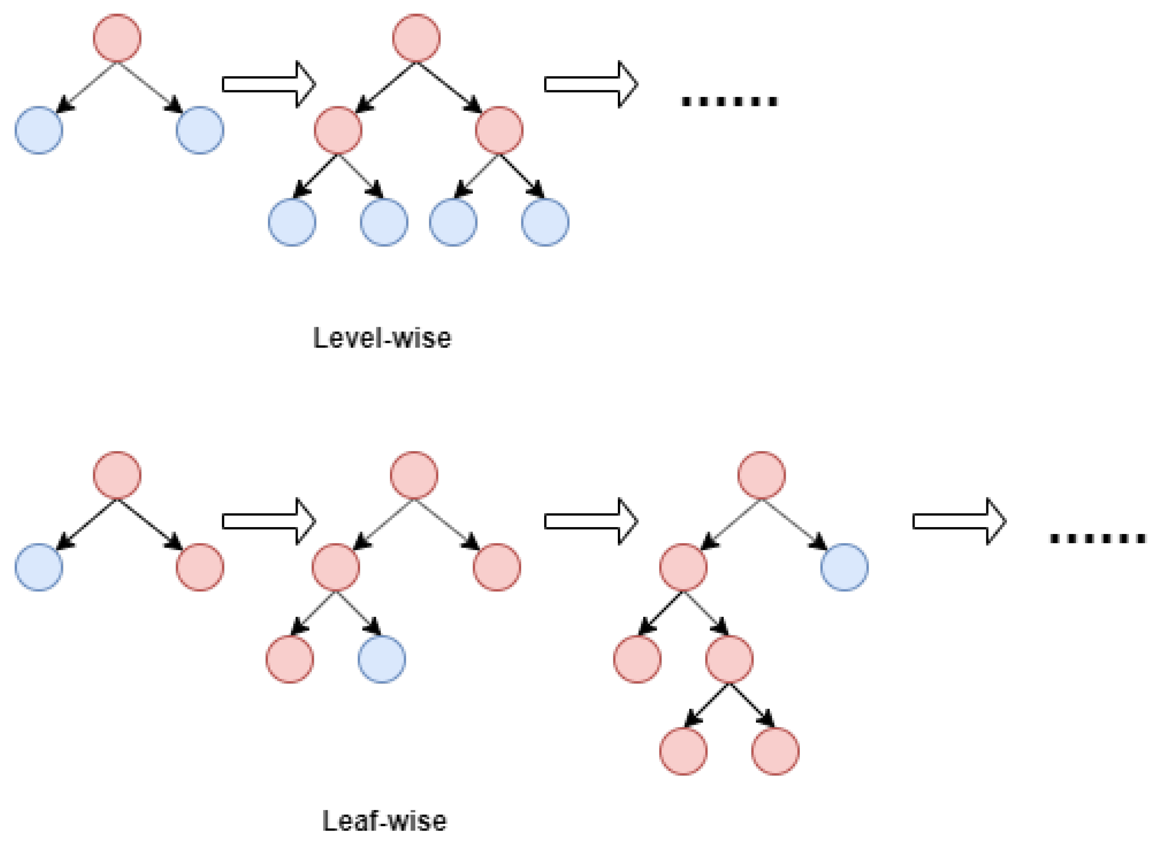
Leafwise growth [27] algorithm: Traditional decision trees such as XGBoost [37] grow levelwise, in which the leaf nodes in the same layer are split at the same time and then pruned. This splitting mode causes much unnecessary computational consumption. LightGBM uses leafwise growth. The model searches for the node with the maximum gain among all the current nodes every time and then splits and iterates repeatedly until the decision tree is completely generated. Leafwise is more efficient than levelwise, but easily generates too deeply, which leads to overfitting. If the decision tree does not have a max depth limit, the tree will continue to split. Under the same number of splits, the decision tree will more deeply generate with leafwise growth. Excessive splitting of the decision tree will make the model learn the information that is not important for the classification, thus reducing the accuracy of the classifier. The algorithm needs to control the maximum depth of the tree to reduce the risk of overfitting. The two algorithms are shown in Figure 2;

(c)

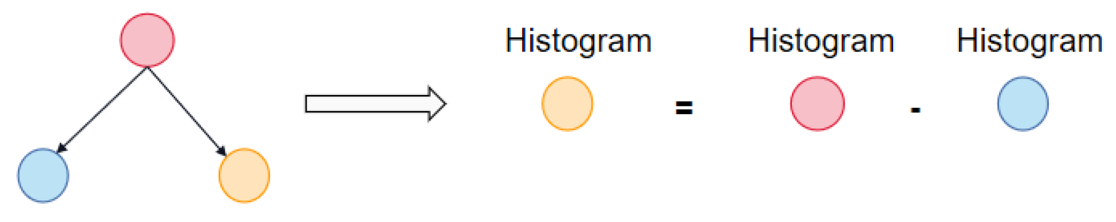
Acceleration of histogram differences: LightGBM accelerates the training process by using the differences of the histograms while constructing them. When splitting, the histogram of the current node is represented by the difference between the histogram of the parent node and the sibling node. This type of acceleration greatly improves the training speed and efficiency [38]. The schematic is shown in Figure 3.

In addition, LightGBM uses the GOSS algorithm [27] to sample data randomly based on gradients and uses the EFB algorithm [27] to further compress features and support efficient parallelism to improve the algorithm’s efficiency without affecting the accuracy.

4. Experimental Process and Analysis

In this study, we selected a total of 567 CV template spectra as positive samples and 20,000 random unlabeled spectra in LAMOST-DR7 as negative samples. The mixed dataset of positive and negative samples was divided into the training set and the testing set according to the ratio of 7:3. Since the wavelength range of each spectra in LAMOST-DR7 is not consistent, to unify the wavelength range, we selected the wavelength range of 4000–8900 Å, which has evident spectral characteristic peaks for sampling, and the sampling points of each spectra were 3473. In machine learning, if the values of different features of samples are large, then the algorithm will prefer the features with larger values in processing, which will mislead the prediction. To enable the algorithm to deal with each feature equally, we normalized the data into [0, 1]. The normalization formula is:

$$S_i=\frac{s_i-{\overline{s}}_i}{\sigma \left(s_i\right)}$$

(11)

where $s_i$ represents the one-dimensional vector formed by spectral flux with wavelength i, ${\overline{s}}_i$ is the mean of $s_i$, and $\sigma$(·) is the standard deviation operator. Next, we constructed the input matrix of the algorithm through the normalized dataset.

4.1. Experimental Metrics

To assess the performance of the models on the dataset, Accuracy, Precision, Recall, the F1-score, and the Receiver Operating Characteristic curve (ROC) were calculated as the experimental metrics, as given below:

$$Accuracy=\frac{TP+TN}{TP+TN+FP+FN}$$

(12)

$$Precision=\frac{TP}{TP+FP}$$

(13)

$$Recall=\frac{TP}{TP+FN}$$

(14)

$$F1-score=\frac{2·Precision·Recall}{Precision+Recall}$$

(15)

where:

(i)

TP means the number of positive samples predicted correctly as CVs;

(ii)

FN means the number of positive samples that not predicted as CVs;

(iii)

FP means the the number of negative samples predicted incorrectly as CVs;

(iv)

TN means the number of negative samples predicted correctly as negative samples.

The ROC curve, which does not depend on the scale of the test set, can evaluate the performance of the model comprehensively. The curve is based on the False Positive Rate (FPR) and the True Positive Rate (TPR). The false positive rate is the ratio of the number of negative samples predicted incorrectly as CVs to the actual number of negative samples. The true positive rate is the ratio of the number of positive samples predicted correctly as CVs to the total number of actual CVs. By adjusting the threshold of the model, we can obtain different (FPR, TPR) points. The ROC curve connects these points as a line. The Area Under the ROC curve is the AUC. The larger the area (AUC) (i.e., the curve is closer to (0, 1)), the better the model classification performance is. If the ROC curve of one model is surrounded by the ROC curve of another model, it is considered that the latter has better performance than the former on this dataset.

4.2. Process Analysis

On the basis of the above dataset, our first step was to train LightGBM classifiers. By using the grid research, we adjusted the best parameters of the learning rate, n_estimators, max_depth, and num_leaves, and obtained the best classifier. The main parameters are defined as follows:

(i)

The learning rate determines whether and when the objective function converges to the local minimum;

(ii)

n_estimators is the number of iterations of the model;

(iii)

max_depth limits the maximum depth of the decision tree;

(iv)

num_leaves limits the maximum number of leaf nodes of the decision tree.

The best main parameters of the LightGBM classifier are shown in

Table 2. Parameter list for LightGBM.

Parameter	Value
learning rate	0.05
n_estimators	372
max_depth	8
num_leaves	40

.

In the second step, we used Accuracy, Precision, Recall, and the F1-score to evaluate the performance of the LightGBM model.

Table 3. Evaluating the indicators of LightGBM.

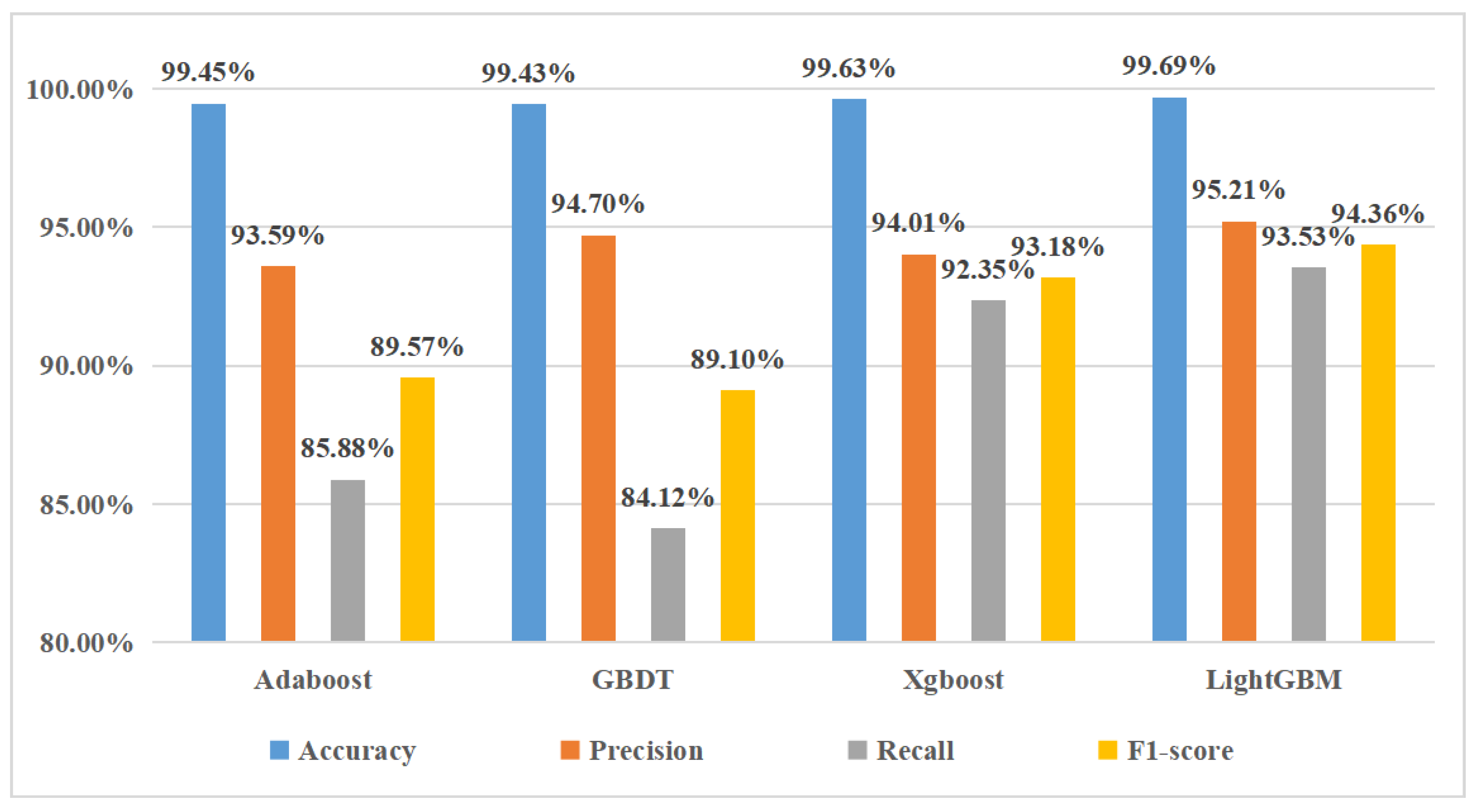
	Accuracy	Precision	Recall	F1-Score
LightGBM	99.69%	95.21%	93.53%	94.36%

shows that LightGBM had a great performance on the testing set. All the indicators of LightGBM were over 90%, and the Accuracy even reached 99.69%.

Moreover, we can obtain a distribution map of the importance score of the spectral features based on the classification model of LightGBM. The importance score is the importance of the features corresponding to the wavelengths to the classification performance in the training process. The higher the importance score, the more important for the classification model the feature is. Figure 4 shows that the importance scores of $H_{\delta }$(4102 Å), $H_{\gamma }$(4340 Å), $H_{\beta }$(4861 Å), $H_{\alpha }$(6563 Å), $HeII$(4685 Å), and $HeI$(5876 Å) were relatively high. Figure 4 shows that LightGBM had better generalization capabilities and could extract the complex features of CV spectra. This result is consistent with the description of the spectral characteristics of CVs [26]. Although there is noise in the spectral data, we focused on the Balmer and He lines in the process of searching for cataclysmic variable candidates. Moreover, LightGBM constructs decision trees based on a combination of multiple features. In the process of each iteration, each split of the decision tree will select a spectral feature with the maximum gain, such as the Balmer and He lines. With the continuous growth and iteration of the decision tree, LightGBM will select multiple spectral features. The single noise, which has little gain in the split, is less selected or not selected in the split. Thus, LightGBM can effectively avoid a single feature from being interfered with by noise and affecting the classification performance. The experimental results also proved this point.

4.3. Comparison of the Models

In this paper, we also trained the AdaBoost [39], GBDT [40], and XGBoost models based on the same training set and tested them on the same test set for the comparison with the LightGBM model. The comparison result is shown in Figure 5.

The results showed that the four models had good performance on spectra classification and the evaluation indicators of all models were over 80%. Compared with the other three models, LightGBM performed best and had the highest Accuracy, Precise, Recall, and F1-score among the four models.

Table 4. Runtimes of the four models.

Model	AdaBoost	GBDT	XGBoost	LightGBM
Time	341.73 s	269.25 s	190.05 s	75.41 s

shows the runtime of the four models, which was calculated from multiple runtimes. The runtime of the LightGBM model was far shorter than those of the other models, and the classification efficiency was high, which is suitable for its promotion for and application to larger-scale spectral data.

Given the imbalance of positive and negative samples, this study also compared the ROC curves of the four models. Figure 6 shows that the ROC curves of AdaBoost, GBDT, and XGBoost are surrounded by the ROC curve of the LightGBM model, and the AUC of LightGBM is largest among all models. This outcome indicated that the LightGBM classifier had a higher accuracy and a stable performance. Hence, the superiority of LightGBM was further proven.

4.4. Experimental Result

This study used the LightGBM classifier to search for CV candidates in LAMOST-DR7, and 225 CV candidates were found. After verification by SIMBAD and the published CV catalogs, there were four new CV candidates including a CV candidate (J020321.98 + 460731.5) in the outburst period, for which the emission nucleus of the Balmer line is clearly visible from its spectra. The list of CV candidates is shown in

Table 5. List of new CV candidates.

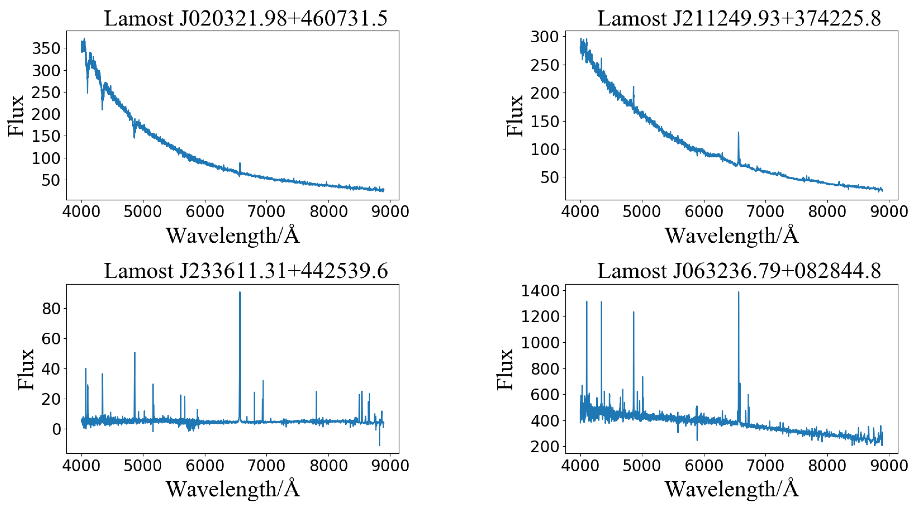
Designation	Obsid	Obsdate	Ra	Dec
J020321.98 + 460731.5	631616056	17 January 2018	30.8415900000	46.1254250000
J211249.93 + 374225.8	593810181	20 October 2017	318.2080800000	37.7071940000
J233611.31 + 442539.6	475914160	3 November 2016	354.0471500000	44.4276800000
J063236.79 + 082844.8	605312123	17 November 2017	98.1533180000	8.4791159000

, and the spectra are shown in Figure 7.

5. Conclusions

A CV star is a type of variable star. There are two different characteristics of the spectra in different periods. Therefore, the spectra of CVs are complex, and conventional methods can not learn these two characteristics at the same time. This study proposed a method to search for CV candidates automatically by using the LightGBM classifier in LAMOST-DR7. The model can extract the potential relationship of CV spectra in quiescent and outburst periods during the training process. By combining multiple features, LightGBM constructs the decision trees and can prevent a single feature from being disturbed by noise, affecting the classification accuracy. Finally, the experiment successfully found four new CV candidates, including a CV candidate in the outburst period, which verifies the accuracy and feasibility of the LightGBM model and enriches the existing CV spectral library. This study also used multiple indicators to compare LightGBM with AdaBoost, GBDT, and XGBoost. The result showed that the evaluation indicators of all models were over 80%, and all indicators of LightGBM were better than those of the other models. In addition, the runtime of LightGBM was much shorter, and the classification efficiency of LightGBM was higher. LightGBM is more suitable for large-scale and high-dimensional spectral data. The successful application of LightGBM in searching for CV candidates also provides a reference for data mining of other rare objects, such as planetary nebulae and HII regions.

References

- Hellier, C. Cataclysmic Variable Stars: How and Why They Vary; Springer: New York, NY, USA, 2001. [Google Scholar]
- Patterson, J. The DQ Herculis stars. Publ. Astron. Soc. Pac. 1994, 106, 209. [Google Scholar] [CrossRef]
- Hack, M.; La Dous, C. Cataclysmic Variables and Related Objects; National Aeronautics and Space Administration, Scientific and Technical: Washington, DC, USA, 1993; Volume 507.
- Sion, E.M. Recent advances on the formation and evolution of white dwarfs. Publ. Astron. Soc. Pac. 1986, 98, 821. [Google Scholar] [CrossRef]
- Warner, B. Cataclysmic Variable Stars, Vol. 28 of Cambridge Astrophysics Series; Cambridge University Press: Cambridge, UK, 1995; Volume 15, p. 20. [Google Scholar]
- Han, X.L.; Zhang, L.Y.; Shi, J.R.; Pi, Q.F.; Lu, H.P.; Zhao, L.B.; Terheide, R.K.; Jiang, L.Y. Cataclysmic variables based on the stellar spectral survey LAMOST DR3. Res. Astron. Astrophys. 2018, 18, 125–146. [Google Scholar] [CrossRef]
- Pan, C.Y.; Dai, Z.B.; Observatories, Y. Investigations on the Observations of Three Types of Periodic Oscillations in Cataclysmic Variables. Acta Astron. Sin. 2019, 60, 35. [Google Scholar]
- Hou, W.; Luo, A.L.; Li, Y.B.; Qin, L. Spectroscopically Identified Cataclysmic Variables from the LAMOST Survey. I. The Sample. Astron. J. 2020, 159, 43. [Google Scholar] [CrossRef]
- Patterson, J. The evolution of cataclysmic and low-mass X-ray binaries. Astrophys. J. Suppl. 1984, 54, 443–493. [Google Scholar] [CrossRef]
- Robinson, E.L. The structure of cataclysmic variables. Annu. Rev. Astron. Astrophys. 1976, 14, 119–142. [Google Scholar] [CrossRef]
- Li, Z.Y. The Observational Properties Of Cataclysmic Variables. Ann. Shanghai Astron. Obs. Chin. Acad. Sci. 1998, 19, 225–229. [Google Scholar]
- Szkody, P.; Anderson, S.F.; Agüeros, M.; Covarrubias, R.; Bentz, M.; Hawley, S.; Margon, B.; Voges, W.; Henden, A.; Knapp, G.R. Cataclysmic variables from the sloan digital sky survey. I. The first results. Astron. J. 2002, 123, 430. [Google Scholar] [CrossRef]
- Szkody, P.; Fraser, O.; Silvestri, N.; Henden, A.; Anderson, S.F.; Frith, J.; Lawton, B.; Owens, E.; Raymond, S.; Schmidt, G. Cataclysmic variables from the sloan digital sky survey. II. The second year. Astron. J. 2003, 126, 1499. [Google Scholar] [CrossRef]
- Szkody, P.; Henden, A.; Fraser, O.; Silvestri, N.; Bochanski, J.; Wolfe, M.A.; Agüeros, M.; Warner, B.; Woudt, P.; Tramposch, J. Cataclysmic Variables from the Sloan Digital Sky Survey. III. The Third Year. Astron. J. 2004, 128, 1882. [Google Scholar] [CrossRef]
- Szkody, P.; Henden, A.; Fraser, O.J.; Silvestri, N.M.; Schmidt, G.D.; Bochanski, J.J.; Wolfe, M.A.; Agüeros, M.; Anderson, S.F.; Mannikko, L. Cataclysmic Variables from Sloan Digital Sky Survey. IV. The Fourth Year (2003). Astron. J. 2005, 129, 2386. [Google Scholar] [CrossRef] [Green Version]
- Szkody, P.; Henden, A.; Agüeros, M.; Anderson, S.F.; Bochanski, J.J.; Knapp, G.R.; Mannikko, L.; Mukadam, A.; Silvestri, N.M.; Schmidt, G.D. Cataclysmic Variables from Sloan Digital Sky Survey. V. The Fifth Year (2004). Astron. J. 2006, 131, 973. [Google Scholar] [CrossRef] [Green Version]
- Szkody, P.; Henden, A.; Mannikko, L.; Mukadam, A.; Schmidt, G.D.; Bochanski, J.J.; Agüeros, M.; Anderson, S.F.; Silvestri, N.M.; Dahab, W.E. Cataclysmic Variables from Sloan Digital Sky Survey. VI. The Sixth Year (2005). Astron. J. 2007, 134, 185. [Google Scholar] [CrossRef] [Green Version]
- Szkody, P.; Anderson, S.F.; Hayden, M.; Kronberg, M.; McGurk, R.; Riecken, T.; Schmidt, G.D.; West, A.A.; Gänsicke, B.T.; Gomez-Moran, A.N. Cataclysmic variables from SDSS. VII. The seventh year (2006). Astron. J. 2009, 137, 4011. [Google Scholar] [CrossRef]
- York, D.G.; Adelman, J.; Anderson, J.E., Jr.; Anderson, S.F.; Annis, J.; Bahcall, N.A.; Bakken, J.A.; Barkhouser, R.; Bastian, S.; Berman, E.; et al. The Sloan Digital Sky Survey: Technical Summary. Astron. J. 2000, 120, 1579. [Google Scholar] [CrossRef]
- Szkody, P.; Anderson, S.F.; Brooks, K.; Gänsicke, B.T.; Kronberg, M.; Riecken, T.; Ross, N.P.; Schmidt, G.D.; Schneider, D.P.; Agüeros, M.A. Cataclysmic variables from the Sloan digital sky survey. VIII. The final year (2007–2008). Astron. J. 2011, 142, 181. [Google Scholar] [CrossRef] [Green Version]
- Djorgovski, S.G.; Drake, A.J.; Mahabal, A.A.; Graham, M.J.; Donalek, C.; Williams, R.; Beshore, E.; Larson, S.M.; Prieto, J.; Catelan, M. The Catalina Real-time Transient Survey. Proc. Int. Astron. Union 2011, 285, 306. [Google Scholar]
- Drake, A.; Gänsicke, B.; Djorgovski, S.; Wils, P.; Mahabal, A.; Graham, M.; Yang, T.C.; Williams, R.; Catelan, M.; Prieto, J.; et al. Cataclysmic variables from the catalina real-time transient survey. Mon. Not. R. Astron. Soc. 2014, 441, 1186–1200. [Google Scholar] [CrossRef] [Green Version]
- Udalski, A. The Optical Gravitational Lensing Experiment. Real Time Data Analysis Systems in the OGLE-III Survey. Acta Astron. 2004, 53, 291–305. [Google Scholar]
- Mróz, P.; Udalski, A.; Poleski, R.; Pietrukowicz, P.; Szymanski, M.; Soszynski, I.; Wyrzykowski, L.; Ulaczyk, K.; Kozlowski, S.; Skowron, J. One thousand new dwarf novae from the OGLE survey. arXiv 2016, arXiv:1601.02617. [Google Scholar]
- Jiang, B.; Luo, A.L.; Zhao, Y.H. Data Mining of Cataclysmic Variables Candidates in Massive Spectra. Spectrosc. Spectr. Anal. 2011, 31, 2278–2282. [Google Scholar]
- Jiang, B.; Luo, A.L.; Zhao, Y.H. Data Mining Approach to Cataclysmic Variables Candidates Based on Random Forest Algorithm. Spectrosc. Spectr. Anal. 2012, 32, 510–513. [Google Scholar]
- Ke, G.L.; Meng, Q.; Finley, T.; Wang, T.F.; Chen, W.; Ma, W.D.; Ye, Q.W.; Liu, T.Y. LightGBM: A highly efficient gradient boosting decision tree. Adv. Neural Inf. Process. Syst. 2017, 30, 3146–3154. [Google Scholar]
- Zhao, G.; Zhao, Y.H.; Chu, Y.Q.; Jing, Y.P.; Deng, L.C. LAMOST spectral survey—An overview. Res. Astron. Astrophys. 2012, 12, 723. [Google Scholar] [CrossRef] [Green Version]
- Cui, X.Q.; Zhao, Y.H.; Chu, Y.Q.; Li, G.P.; Li, Q.; Zhang, L.P.; Su, H.J.; Yao, Z.Q.; Wang, Y.N.; Xing, X.Z. The large sky area multi-object fiber spectroscopic telescope (LAMOST). Res. Astron. Astrophys. 2012, 12, 1197. [Google Scholar] [CrossRef]
- Luo, A.L.; Zhang, H.T.; Zhao, Y.H.; Zhao, G.; Cui, X.Q.; Li, G.P.; Chu, Y.Q.; Shi, J.R.; Wang, G.; Zhang, J.N. Data release of the LAMOST pilot survey. Res. Astron. Astrophys. 2012, 12, 1243. [Google Scholar] [CrossRef]
- Luo, A.L.; Zhang, H.T.; Zhao, Y.H.; Zhao, G.; Deng, L.C.; Liu, X.W.; Jing, Y.P.; Wang, G.; Zhang, H.T.; Shi, J.R.; et al. The first data release (DR1) of the LAMOST regular survey. Res. Astron. Astrophys. 2015, 15, 1095. [Google Scholar] [CrossRef]
- Chen, S.X.; Sun, W.M.; Kong, X. Difference Analysis of LAMOST Stellar Spectrum and Kurucz Model Based on Grid Clustering. Spectrosc. Spectr. Anal. 2017, 37, 1951–1954. [Google Scholar]
- Pulicherla, P.; Kumar, T.; Abbaraju, N.; Khatri, H. Job Shifting Prediction and Analysis Using Machine Learning. J. Phys. Conf. Ser. 2019, 1228, 012056. [Google Scholar] [CrossRef]
- Wang, D.; Yang, Z.; Yi, Z. An Effective miRNA Classification Method in Breast Cancer Patients. In Proceedings of the 2017 International Conference on Computational Biology and Bioinformatics, Newark, NJ, USA, 18–20 October 2017. [Google Scholar]
- Sun, X.; Liu, M.; Sima, Z. A novel cryptocurrency price trend forecasting model based on LightGBM. Financ. Res. Lett. 2020, 32, 101084. [Google Scholar] [CrossRef]
- Jain, A.; Saini, M.; Kumar, M. Greedy Algorithm. J. Adv. Res. Comput. Sci. Eng. 2015, 2, 11015. [Google Scholar]
- Chen, T.; Guestrin, C. XGBoost: A scalable tree boosting system. In Proceedings of the 22nd ACM Sigkdd International Conference on Knowledge Discovery and Data Mining, San Francisco, CA, USA, 13–17 August 2016; pp. 785–794. [Google Scholar]
- Jing, W.; Yi, Z.-P.; Yue, L.-L.; Dong, H.-F.; Pan, J.-C.; Bu, Y.-D. Spectral Classification of M-Type Stars Based on Ensemble Tree Models. Spectrosc. Spectr. Anal. 2019, 39, 2288–2292. [Google Scholar]
- Freund, Y.; Schapire, R.E. A decision-theoretic generalization of on-line learning and an application to boosting. J. Comput. Syst. Sci. 1997, 55, 119–139. [Google Scholar] [CrossRef] [Green Version]
- Friedman, J.H. Greedy function approximation: A gradient boosting machine. Ann. Stat. 2001, 29, 1189–1232. [Google Scholar] [CrossRef]