Article

Three-Dimensional MHD Modeling of Interplanetary Solar Wind Using Self-Consistent Boundary Condition Obtained from Multiple Observations and Machine Learning

1
National Space Science Center, Chinese Academy of Sciences, Beijing 100190, China
2
College of Earth and Planetary Sciences, University of Chinese Academy of Sciences, Beijing 100049, China
*
Author to whom correspondence should be addressed.
Universe 2021, 7(10), 371; https://doi.org/10.3390/universe7100371
Submission received: 31 August 2021 / Revised: 27 September 2021 / Accepted: 1 October 2021 / Published: 4 October 2021
(This article belongs to the Special Issue Plasma Physics in Astronomy)

Abstract

:
Three-dimensional (3-d) magnetohydrodynamics (MHD) modeling is a key method for studying the interplanetary solar wind. In this paper, we introduce a new 3-d MHD solar wind model driven by the self-consistent boundary condition obtained from multiple observations and the Artificial Neural Network (ANN) machine learning technique. At the inner boundary, the magnetic field is derived using the magnetogram and potential field source surface extrapolation; the electron density is derived from the polarized brightness (pB) observations, the velocity can be deduced by an ANN using both the magnetogram and pB observations, and the temperature is derived from the magnetic field and electron density by a self-consistent method. Then, the 3-d interplanetary solar wind from CR2057 to CR2062 is modeled by the new model with the self-consistent boundary conditions. The modeling results present various observational characteristics at different latitudes, and are in better agreement with both the OMNI and Ulysses observations compared to our previous MHD model based only on photospheric magnetic field observations.

1. Introduction

Magnetohydrodynamic (MHD) modeling is an important method for space plasma physics research and space weather prediction. In the research field of heliophysics, MHD models have been widely used in the studies of coronal–interplanetary solar wind, the propagation of coronal mass ejections (CMEs), and their interaction process [1]. Obtaining the realistic three-dimensional (3-d) solar wind plasma and magnetic field environment is a significant foundation for studying and predicting the propagation process of catastrophic space weather events such as CMEs and solar energetic particles (SEPs) [2,3,4,5,6,7,8,9]. Therefore, the development of a realistic 3-d MHD model for the interplanetary solar wind has great theoretical and practical value.
Different research groups have developed a few reasonable 3-d MHD solar wind modeling systems with relatively good performance at present, for example, the space weather modeling framework (SWMF) developed by the Center for Space Environment Modeling (CSEM) at University of Michigan [10], the Coronal-Heliosphere (CORHEL) model developed by the Center for Integrated Space Weather Modeling (CISM) at Boston University [11,12], the WSA-ENLIL model utilized by the space weather prediction center at National Oceanic and Atmospheric Administration (NOAA) [13], the SIP-CESE model and the COIN-TVD model developed by the National Space Science Center at Chinese Academy of Sciences [14,15,16], the EUHFORIA model developed by the European research community [17], and some models developed by other researchers [18,19,20,21].
Considering solar wind propagates to the interplanetary space through a complex heating and accelerating process at the inner corona, the current 3-d MHD solar wind models usually divide the solar–interplanetary space into two computational regions and deal with them by different methods [22]. One kind of model computes both the coronal and interplanetary regions by the physics-based MHD algorithm, and deals with the heating and accelerating process in the corona by adding mathematical terms to the MHD equations, such as the SWMF model and the SIP-CESE model. The other kinds of model deals with the coronal region by semi-empirical models, and only compute the interplanetary region by the MHD algorism. The second kind of model generally sets the inner boundary of MHD computational region beyond the Alfven critical point (around 0.1 AU from the Sun), and determines the inner boundary conditions with semi-empirical methods, such as the WSA-ENLIL model and the EUFORIA model.
The plasma β is the ratio of the plasma pressure to the magnetic pressure. Due to the plasma β << 1 in the corona, the numerical computation of the first kind of solar wind models requires a large amount of computing resources, while the second kind of model can save the computational cost of the corona and improve the computational efficiency for interplanetary solar wind greatly. Since the heating and accelerating mechanisms of the solar wind have not been totally revealed, the models based on empirical boundary conditions are no less effective than the models fully based on physical equations in reproducing large-scale structures of interplanetary solar wind, as a study that compared the two kinds of models in detail presented [23]. Therefore, the interplanetary solar wind model based on empirical boundary conditions has important value in solar wind prediction in terms of both efficiency and accuracy. For example, the WSA-ENLIL model based on the WSA empirical function for solar wind velocity has been utilized as an operational model by the SWPC/NOAA.
The performance of the hybrid empirical-MHD solar wind model is highly dependent on the initial boundary conditions used to solve the MHD equations, thus the realistic initial boundary conditions are significant to the simulation accuracy of the interplanetary solar wind [24,25,26,27,28,29]. Since the magnetic field is the main factor controlling the motion of solar wind plasma, most advanced solar wind MHD models utilize observational data of the photospheric magnetic field and some theoretical extrapolation models to obtain the initial boundary conditions of the magnetic field. For example, the potential field source surface (PFSS) model can extrapolate the coronal magnetic field from the photospheric magnetograms, and is widely used in current solar wind models. The boundary condition of velocity is usually given by the WSA model [30,31,32] based on an empirical relation between solar wind velocity and magnetic field expansion factor. In addition, the initial boundary conditions of density and temperature are generally derived by the assumption of constant momentum flux and the total pressure (sum of thermal and magnetic pressures) balance [19,28,33,34]. Thus, these two parameters are closely related to the derived magnetic field and velocity.
However, the coronal magnetic field extrapolated through theoretical models with some ideal assumptions, such as the potential field assumption, may be biased from the reality. Therefore, some additional types of observational data can be considered to improve the boundary conditions of solar wind MHD models. For example, some recent studies have tried to correct the coronal magnetic field extrapolated from the PFSS model by the white light brightness observation, according to the magnetic freezing effect of the solar wind plasma [35,36]. In addition, the empirical functions for solar wind velocity in the WSA model are derived only from ecliptic solar wind observations, so it may have uncertainties for providing the global distribution. Since the global structure of solar wind velocity can be obtained from the interplanetary scintillation (IPS) observations, some researchers have utilized the IPS data to give the boundary conditions of solar wind MHD models [25,37,38,39]. However, the IPS observation stations cannot operate every winter due to thick snow, and the data also could not cover all the global regions for other seasons due to the lack of proper radio sources [40].
With the development of computational technology and the accumulation of observational data, machine learning techniques have been introduced to predict the solar wind condition in recent years. For example, different machine learning algorisms have been utilized to predict the solar wind speed near the Earth [41,42]. However, these models can only give the prediction of solar wind speed near the Earth, and cannot give the 3-d distribution of all the solar wind parameters. In our recent work [43], we have developed a new method using multiple observations and the artificial neural network (ANN) machine learning technique to obtain the self-consistent global distribution of the magnetic field, electron density, flow velocity and plasma temperature on the coronal source surface. We established an empirical model for solar wind velocity based on the magnetic field properties and the electron density derived from the observations of photospheric magnetogram and polarized brightness. The new empirical correlation is determined from global observations at all latitudes as it utilized the IPS solar wind velocity data. The plasma temperature distribution is deduced by solving a 1D MHD system at the source surface. Therefore, the global distribution of different solar wind parameters is deduced self-consistently based on multiple observational data.
In this paper, we introduce a new 3-d MHD interplanetary solar wind model that coupled the method of obtaining self-consistent global distribution of solar wind parameters at the coronal source surface [43] and the interplanetary total variation diminishing (IN-TVD) MHD solar wind model [29]. By analyzing the modeled global structure of solar wind plasma and magnetic field, the new model is validated. Then, the modeling results are compared with in situ observations both at the ecliptic plane and at higher latitudes along the Ulysses spacecraft trajectory. In addition, the comparison with our previous MHD model shows the advantages of the multiple observation driven model.
The outline of this paper is as follows: in Section 2, we describe the data and methods that we used to establish the new MHD model. In Section 3, we first make analyses for the modeled global structure of different solar wind parameters during one Carrington rotation (CR), then we validate the model by comparing the modeling results with the Ulysses observations for six CRs from CR 2057 to CR 2062, i.e., the period from May 24th to Nov 4th of 2007. In Section 4, we discuss the results and draw some conclusions.

2. Materials and Methods

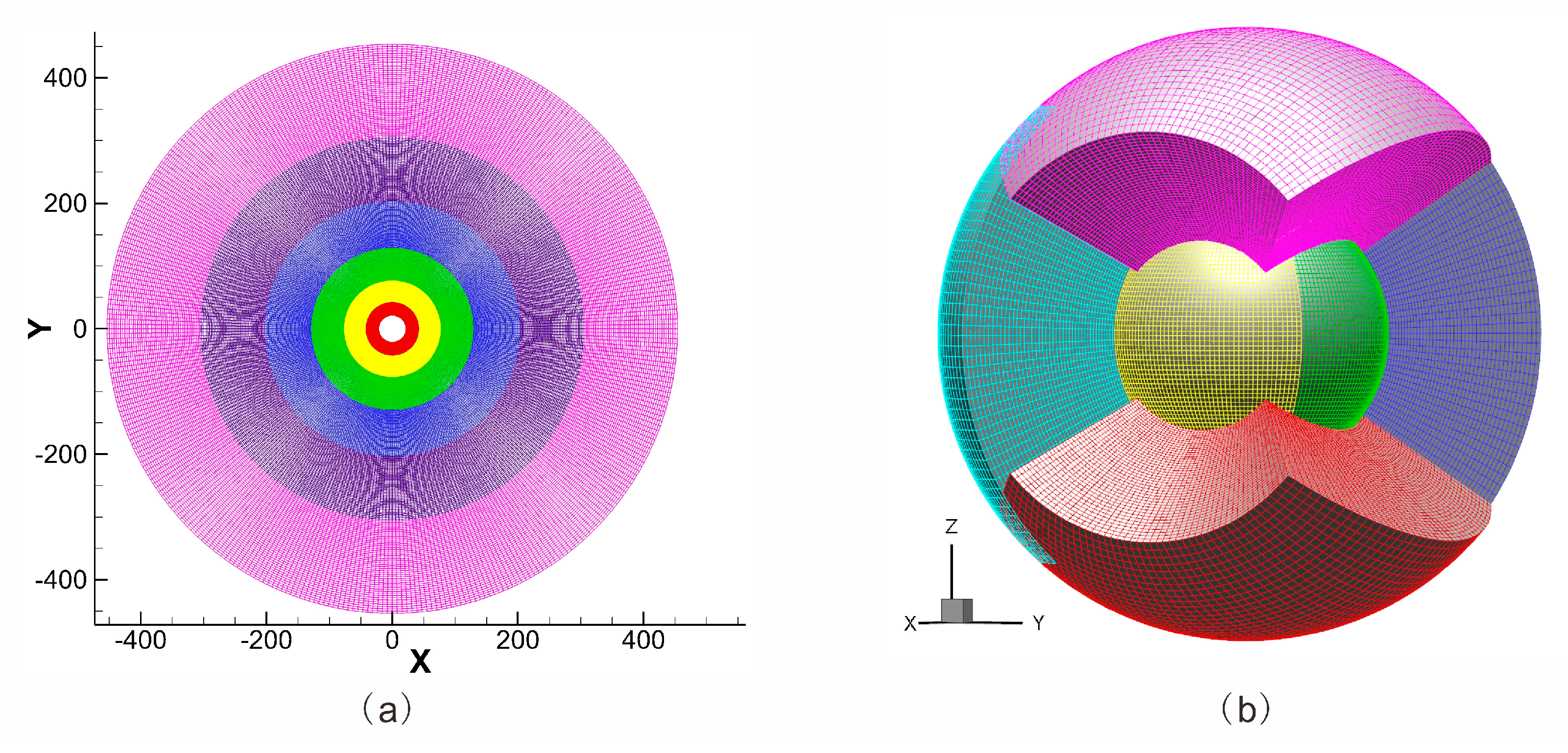
2.1. The MHD Numerical Model

Our interplanetary solar wind model is based on the 3-d ideal MHD equations. Because the solar wind and interplanetary magnetic field are rigidly co-rotating with the Sun, a co-rotating coordinate system can facilitate the processing of the bottom boundary conditions. In the co-rotating coordinates, the ideal MHD equations in the conservation form can be written as:
ρ t + ρ V = 0 ,
ρ V t + p + B 2 2 μ 0 I + ρ V V B B μ 0 = ρ G M s r 3 r + V f ,
B t + V B B V = 0   ,
p t + p V = γ 1 p V ,
where the physical parameters to be solved are the plasma density ρ , pressure p , velocity vector V and magnetic field vector B . Equation (1) is the continuity equation. Equation (2) is the momentum equation, where μ 0 is the vacuum permeability, I denotes the unit tensor, G is the universal gravitational constant, M s is the mass of the Sun, ω is the angular velocity of the solar rotation, and f = ω × ω × r + 2 ω × V is the centrifugal force introduced because of the adoption of the co-rotating coordinate system. Equation (3) is the simplified electromagnetic equation considering the ideal MHD condition. Equation (4) is the pressure equation used instead of the energy equation, where γ is the polytrophic index. The use of pressure equation is beneficial to ensure the stability of the numerical scheme [13].
In our model, the Lax–Friedrich finite difference scheme is used with the total variation diminishing (TVD) feature to solve the above 3-d time-dependent MHD equations in all the computational regions. In addition, since the numerical calculation cannot guarantee the physical condition that the divergence of the magnetic field is zero everywhere, so the divergence of the magnetic field may accumulate at some places and lead to the collapse of the calculation, and some methods have to be adopted to limit the divergence of the magnetic field. In this paper, we have adopted the diffusion method [44,45], which added a diffusion term to the equation to make the magnetic field divergence generated by numerical calculation spread rapidly to the whole calculation domain, so that the stability of the calculation can be ensured. Other details of the numerical scheme can be referred to the previous papers [15,46].
Our calculation domain is set to be from 0.1 AU to about 2 AU from the Sun’s center, exactly [21.5 R s , 450 R s ] in units of solar radius ( R s ). The meshes in the radial direction are divided by equal ratio, so the meshes become larger with the increase in heliocentric distance. The radial mesh size increases gradually from 0.37 R s to 3.6 R s . The allowable time step will be larger as the grid is larger, according to the Courant–Friedrichs–Lewy (CFL) conditions of numerical calculation. Therefore, we divide the whole computing space into six regions in the radial direction, and each region uses its own allowable time step, so that asynchronous parallel method can be adopted in the calculation to save the calculation time [15]. The division of radial grids is shown in Figure 1a. Different colors represent six different regions divided radially. There are 48 grid point in each region, and 4 of them overlap with the nearby region. The number of grids in the radial direction can be adjusted as needed to obtain the appropriate calculation area.
On the spherical shell of our computation domain, a six-component grid system is adopted to avoid the singularity in the spherical coordinate system and facilitate parallel computing with high performance. The six-component grid system consists of six identical regions, four of which are arranged in order along the longitude in the middle and low latitudes, and the other two are used to cover the North and South poles. Each component intersects with the nearby ones to cover an entire sphere. Figure 1b shows a diagram of the six-component grid systems in 3-d with each component represented by a different color.
In the six-component grid system, each component has an independent coordinate, and the coordinate range of each region is as follows:
π 4 Δ θ 3 π 4 + Δ 3 π 4 Δ ϕ 5 π 4 + Δ ,
where Δ represents the size of the overlap between the components on a spherical shell. Each component is divided according to the following rules:
θ j = θ m i n + j 1 Δ θ ,   Δ θ = θ m a x θ m i n n 1 ,
ϕ k = ϕ m i n + k 1 Δ ϕ ,   Δ ϕ = ϕ m a x ϕ m i n n 1 ,
where n is the number of grids in the direction of θ or ϕ . In this work, we adopted a mesh with the resolution of 1° × 1° on a sphere, and the overlapping parts of different components are set to 7 grids, so the value of n is 97. During the calculation process, the values of physical parameters for the inner grids of each component are solved by the numerical scheme, and the values on the boundary of each components are obtained by interpolation of the adjacent overlapping grids.

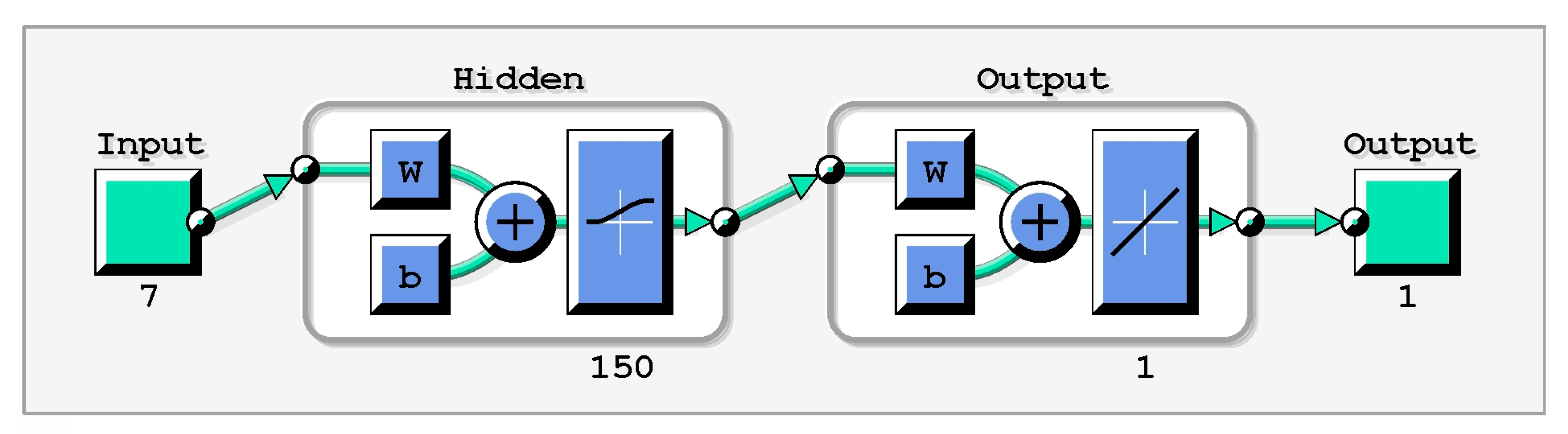
2.2. Boundary Conditions Obtained from Multiple Observations and Machine Learning

As mentioned above, the inner boundary of the calculation domain in this paper is located at 21.5 R s , which belongs to the supersonic and super-Alfven-velocity region. Thus, all the characteristic waves on the inner boundary are pointed to the calculation region, so all the physical values in the MHD equations need to be set empirically. The outer boundary adopts no reflection condition, which can be obtained by linear extrapolation of the points in the calculation region.
If realistic boundary conditions are given to the MHD model, the simulated interplanetary solar wind can be well consistent with actual observations. In order to provide a more realistic inner boundary, here we try to obtain the global distribution of various physical parameters using multiple observational data. Since there is no directly available interplanetary observation data at the inner boundary location, we firstly determine the global distribution of the physical parameters at the coronal source surface (2.5 R s ) using the observational data, and then extrapolate the global distributions to the inner boundary of the MHD model according to the Parker spiral [47]. The following describes how the boundary conditions for magnetic field, density, velocity, and temperature are given based on multiple observations.
Our boundary condition of radial magnetic field is given by the PFSS model [48,49], which can extrapolate the coronal magnetic field structure using the observational data of photospheric magnetograms. Although the PFSS model is relatively simple, it can still predict the polarity of the interplanetary magnetic field well [50], so it is commonly used in a lot of solar wind models. Currently, there are many data sources for the photospheric magnetograms data. According to a comparative study [51,52], we used the data provided by NSO/GONG (http://gong.nso.edu/, accessed on 30 September 2021). Previous studies have demonstrated that the nondipole harmonics of the solar magnetic field can be significant [53]. In this paper, we use a truncation number of 11 for the spherical harmonic expansion in the PFSS model. After the calculation of the magnetic field intensity, we can also obtain some other magnetic characteristic parameters by tracing field lines. The expansion factor f s on the source surface can be derived by the function:
f s = B 0 B s s R 0 R s s 2 ,
where B 0 and B s s are the magnetic field strength at the photosphere and at the source surface, respectively. The parameter θ b is defined as the minimum angular distance between an open field foot point and its nearest coronal hole boundary. The f s and θ b are good indicators for solar wind speed as they are both used in the WSA model.
In addition, we define L m as the latitude difference between a point at the source surface and the heliospheric current sheet (HCS), i.e., the magnetic latitude. The L m is also well related to the solar wind structure, as has been studied by many researchers [54,55,56]. Another feature we derived is the latitude of the magnetic foot-point (defined as L 0 ), since it may also have a relation with the solar wind velocity [57]. The six magnetic field features named B s s ,   B 0 , f s , θ b ,   L m and L 0 which are obtained from the PFSS model were utilized to predict the solar wind speed at 1AU in our previous paper, and achieved a good performance[58]. Thus, we intend to use these features to derive the global distribution of solar wind velocity in this study.
During the propagation of solar wind in interplanetary space, the dynamic pressure ( 1 2 ρ V 2 ) dominates the plasma flow in the region with a weak magnetic field. Thus, it is very necessary to give a reasonable density boundary condition for the 3-d MHD solar wind model. According to the Thomson scattering theory, the coronal electron density can be determined from the white light polarization brightness (pB) observation. Therefore, we obtain the global distribution of electron density at the source surface using the pB data from LASCO/C2 coronagraph and a coronal electron density inversion methods developed by Van de Hulst et al. [59]. Although the LASCO/C3 coronagraph can provide observations at the inner boundary location of our model directly, it cannot be used to invert the electron density distribution, because only the pB observation at low corona can avoid the noise caused by the interplanetary stray light [60].
The boundary condition of solar wind radial velocity is very important in solar wind MHD modeling, because the interaction between high and low velocity flows during the propagation of interplanetary solar wind has a great influence on the evolution of all other solar wind parameters. The current MHD solar wind model generally gives the radial velocity boundary value by the empirical WSA model, which can be expressed in the following formula:
V r = V s + V f 1 + f s a 1   1 0.8 exp θ b a 2 a 3 a 4 ,
where f s is the expansion factor, θ b is the angular distance between the foot point of the magnetic field line and the coronal hole boundary, V s and V f are free parameters used to define the minimum and maximum velocities, and a 1 to a 4 is the free parameters that control the influence of f s and θ b . There are variants of similar formula used in different studies [23,30,61], and we chose the above function because it has reduced free parameters and was validated in our previous study [29]. As mentioned above, the empirical formula of WSA velocity is obtained from the in situ observational data at 1AU in the ecliptic, so the initial boundary conditions of the high latitude region given by the WSA formula may have uncertainties. Moreover, the WSA model only relies on the photospheric magnetic observation. Therefore, it may be better if some other types of observations can be added to constrain the value of the velocity. For these reasons, we have used an artificial neural network (ANN) machine learning technique to establish an empirical relationship among the source surface velocity, six magnetic field parameters based on photospheric magnetic observations and the electron density inverted from pB observations. The new empirical relationship was established using IPS observations of global velocity, so it could be more reasonable than the WSA formula at high latitudes. The ANN model we used is a feed forward network with three layers, including the input layer, the hidden layer and the output layer. The architecture of our ANN model is shown in Figure 2.
The calculation of the ANN can be expressed as follows:
y =   g   b 0 + j = 1 n v j   f j b j + i = 1 m w j i x i ,
where x i is the input features; w j i is the weights between the neuron i of input layer and node j of hidden layer, v j are the weights between the hidden layer and the output; b j and b 0 represent the biases; and y is the target output. Besides, f is a bipolar sigmoid nonlinear activation function used in the hidden layer, and g is a linear function applied for the output layer. The function of f is:
f x = e x 1 + e x .
As shown in Figure 2, we use seven features derived from multiple observations as input and 150 neurons in the hidden layer. Using the above method, we can obtain a velocity boundary condition that are related to both photospheric magnetic observations and coronal pB observations. Figure 3 shows the comparison of (a) the IPS observed solar wind velocity distribution, (b) the ANN model derived velocity distribution, and (c) the WSA model derived velocity distribution during CR2057 to CR2062. We use this period to validate our model because there are few CMEs during this period, so it is proper to examine the model performance for background solar wind.
Our temperature boundary condition is derived by a self-consistent approach based on the already obtained magnetic field intensity and density distributions. It assumes that solar wind plasma satisfies the ideal gas conditions and the statistical results for the constant thermal pressure and plasma beta β at different regions, which can be presented as the following:
p = 2 N R T
β B = 8 π p / B 2
where T is the temperature, N is the density, p is the dynamical pressure, B is the magnetic field intensity, and the value of plasma β is given by:
β = C B 2       current sheet region β c                     other region
and the value of β c and C are given empirically according to the previous study[62]. Since the magnetic field and density are derived from photospheric magnetograms and pB brightness observations, respectively, the temperature computed from them is also related to the two kinds of observations self-consistently.
In addition, the longitudinal and latitudinal components of the magnetic field vector and velocity vector are given according to the corotation as follows:
V θ = 0 V ϕ = ω R i n sin θ
B θ = 0 B ϕ = ω R i n sin θ V r B r
Above all, we have obtained the boundary conditions of all the solar wind physical parameters according to three kinds of observational data, including the photospheric magnetogram, the pB brightness and the IPS velocity data. Then, we can drive the 3-d MHD model introduced in Section 2.1 and achieve the steady-state solution of the 3-d interplanetary solar wind after sufficient time relaxation iteration.
The left column of Figure 4 shows the global distributions of (a) radial velocity, (b) electron density, (c) temperature and (d) radial magnetic field at the inner boundary of our 3-d MHD model obtained from multiple observations and the ANN technique during CR2062. The right column is a comparison with the inner boundary condition based solely on the the WSA model, which we previously used. As the figure showed, the heliospheric current sheet during CR2062 is mainly distributed in low latitude near the equator and is well presented by both methods. However, the global distributions of density and temperature presented in the right column have exactly the same distribution structure with the velocity, while the global distribution of velocity, density and temperature in the left column have many more longitudinal and latitudinal variations, especially for the regions at the high latitudes.

3. Results

Utilizing the new 3-d MHD interplanetary model driven by multiple observations and ANN, we simulated the 3D interplanetary background solar wind during six CRs, which are CR2057 to CR2062. The Ulysses spacecraft had experienced its third fast passage from the solar south to the north, so we could examine the modeling performance at high latitude during this period. Besides, this period was in the year 2007, which is close to the minimum of the 23rd solar cycle, so there were few coronal mass ejections, meaning this time periods would be very suitable for the verification of a background solar wind model.

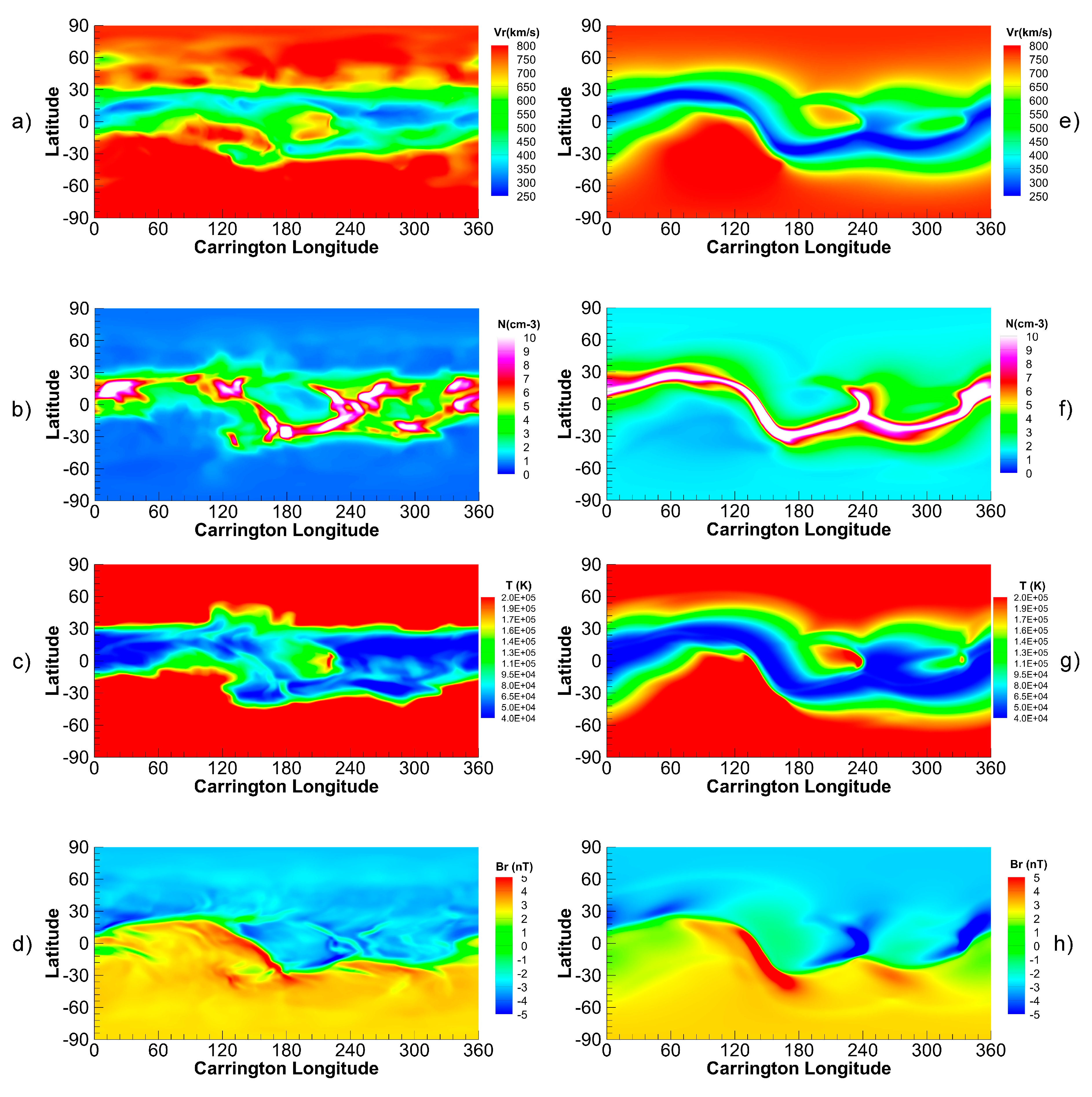
3.1. Analyses of the Modeled Solar Wind Parameters at 1AU

Firstly, we analyzed the modeling results for the global distribution of different solar wind parameters at 1AU during CR2062 as an example.
The left column of Figure 5 shows the global distribution of the interplanetary solar wind parameters at 1AU during CR2062 simulated by the MHD model with our new boundary condition settings. From a comprehensive view of various physical parameters, we can see that in the polar region the velocity is higher, the density is lower, the temperature is higher and the magnetic field is also higher than that in the equatorial region. These characteristics are consistent with the actual observation of large-scale solar wind structures near the minimum activity years in a solar cycle.
By comparison with Figure 4, it can be found that all the solar wind parameters at 1AU had obvious changes compared with the inner boundary. The magnetic field and density at low latitudes showed some inhomogeneous structures due to the interaction between high and low velocity flows, and a few sudden increases emerged due to the compression effects. Besides, the average solar wind speed increased by tens of km/s while the magnetic field and temperature decreased exponentially relative to the inner boundary. This means that when the solar wind travels through interplanetary space, the magnetic energy and internal energy are converted into kinetic energy. In addition, we can intuitively see that the large-scale configuration of all the solar wind parameters at 1AU is shifted to the left about 50 degree in the longitudinal direction relative to the inner boundary, which is due to the co-rotation effect of the solar wind [47].
The right column of Figure 5 shows the global distribution of solar wind parameters at 1AU during CR2062 simulated by the MHD model with our previous boundary condition treatment [29]. The comparison between the left and right columns in Figure 5 shows the modeling results from both models are similar on the large scale, but the new model driven by multiple observations presents more small variations for all the solar wind parameters. In the right column, the values of solar wind plasma parameters along the heliospheric current sheet are equal, while in the left column the values can be different. For example, the densities along the heliospheric current sheet are all above 10 cm−3 according to the results of our previous model, while the new model indicates the density can be less than 10 cm−3. Besides, there are more complex distributions of the parameters at high latitude in the left column. For example, the velocity value is almost the same above 60 degrees according to the result of our previous model, while the new model shows some variations.
In order to examine if the small scale variations simulated by our new MHD model are closer to the actual solar wind environment than the previous model, we compared the modeling results with the in situ observations at 1AU provided by OMNIweb (http://omniweb.gsfc.nasa.gov, accessed on 30 September 2021), and the results are shown in Figure 6. and Table 1.
Figure 6 shows the comparison of our MHD simulation results of solar wind (a) velocity, (b) density, (c) temperature and (d) radial interplanetary magnetic field (IMF) at 1AU with OMNI hourly averaged in situ observational data. The blue lines in Figure 6 show the results from the new model driven by multiple observations and ANN (MHD1), and the cyan lines present the results from our previous MHD model driven by the WSA-based boundary condition (MHD2). The overall trend of all simulated solar wind parameters at 1AU is generally in agreement with the observed value for both the MHD models. The two high-speed flows larger than 400 km/s are relatively accurate. The simulated values of density are generally consistent with the observation, but some peak values are missed. The two periods of temperature simulation values greater than 105 K are generally in agreement with the OMNI observations. The radial magnetic field also agrees with the observations at large scale, but the small fluctuations cannot be simulated by both the MHD models since they may come from the turbulence of the solar wind. We can see intuitively that the lines of the new model are closer to the observations.
Table 1 presents the correlation coefficient (CC) and the root mean squared error (RMSE) between the MHD models and the OMNI observation. We can see that both the MHD models performed well, especially for the solar wind velocity. Additionally, all the parameters simulated by the new model were more accurate than the previous model quantitatively for both CC and RMSE.

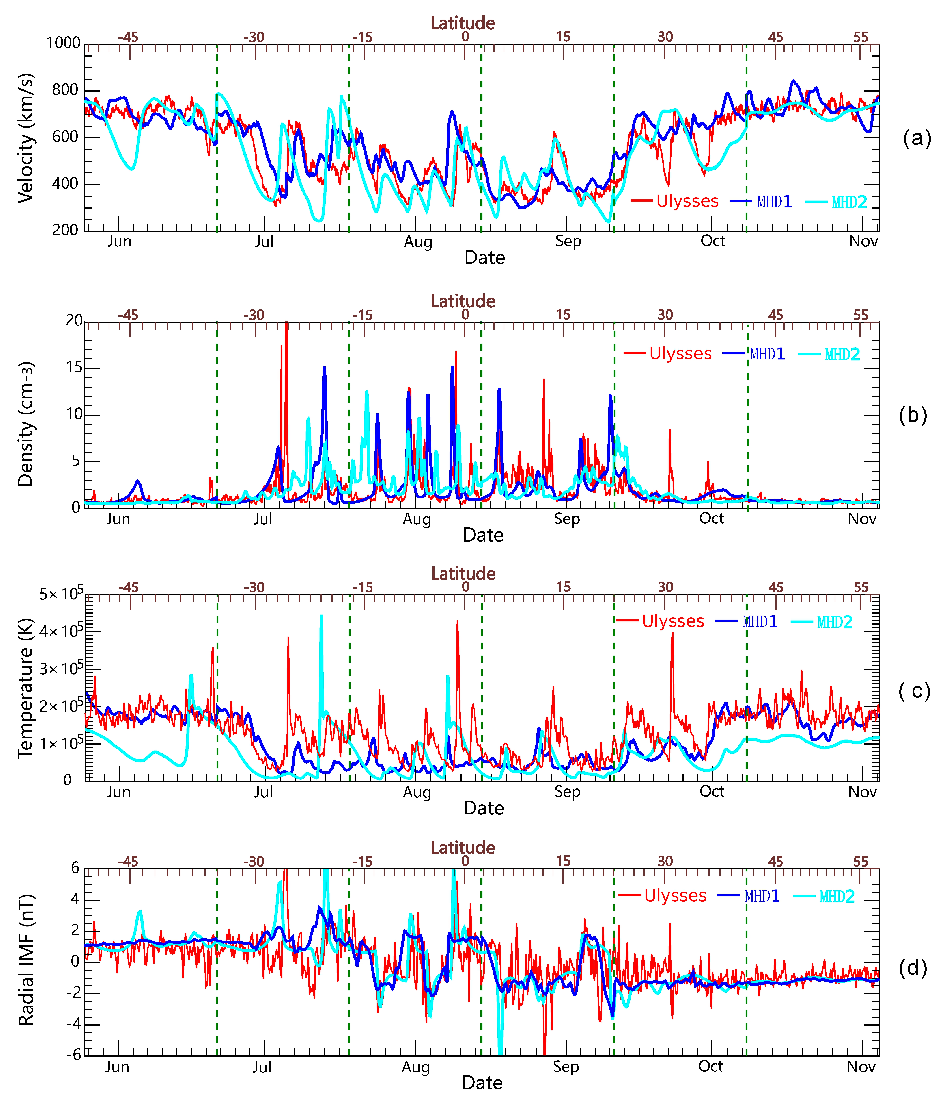
3.2. Comparison with the Ulysses Observation

Comparison between the modeling results and the OMNI in situ observational data at 1AU can only verify the performance of our MHD model on the equatorial plane. In order to further verify the performance of the model at high latitudes, we also compared the results with the observation data of Ulysses. The trajectory of Ulysses spacecraft during CR2057 to CR2062 is shown in Figure 7 as the black curve. The background is the modeled 3-d distribution of velocity during CR2062.
We can see that the Ulysses passed a large latitude range from the Southern Hemisphere to the Northern Hemisphere during CR2057 to CR2062, which is very suitable for comparison with our simulation results at high latitudes. The cone-shaped zones with a reduced speed that can be seen in the polar regions may reflect the presence of conic polar current sheets, which are introduced by a previous research [63].
Figure 8 presents the solar wind parameters simulated by the MHD models and the six-hour averaged in situ observational data from Ulysses. The x axis at the bottom of each panel is the date of the year 2007, and the x axis at the top of each panel is the latitude of the Ulysses spacecraft. The green dashed lines are used to separate the six CRs. We can see that Ulysses traveled from about -50 degrees to above 55 degrees during this period.
Firstly, we examined the general trend over the whole period, and found that both the MHD models indicate that the solar wind velocity and temperature increase with the increase in latitude, while the density decreases with the increase in latitude, which is generally in agreement with the observed characteristics.
Then, if we focus on the latitudes above ±15 degree, the modeling results of our new MHD model coincide with the Ulysses observations better than the previous MHD model for all the solar wind parameters, intuitively. The most obvious improvement is in the temperature at high latitudes, since both the observation and the new MHD model presented the temperature as around 2 × 10 5 below −30 latitude degrees and above 35 degrees, but the previous model presented much lower values. However, the two large dips in speed and the corresponding impulses of density observed by Ulysses during late September to the beginning of October in Figure 8a,b were not well reproduced by both our MHD models. According to the theoretical studies on the quasi-stationary current sheets [64,65], these differences might be caused by the large-scale current sheets at mid-heliolatitudes that are not reproduced by our models, as we can see the inversions of the radial magnetic field direction are only presented by the observational data in Figure 8d.
In order to validate the modeling results more quantitatively, we also calculated the CC and RMSE between the MHD models and the OMNI observation. Overall, both the MHD models perform well, but the solar wind parameters simulated by the new model are more accurate than the previous model.
From the comparison of Table 1 and Table 2, we can find that the metrics of the new MHD model using multiple observations and ANN technique stay nearly the same as at 1AU on the ecliptic plane as at high latitudes, indicating that the model can properly reproduce the solar wind plasma and magnetic field structures globally.

4. Discussion and Conclusions

In this paper, we introduced a new 3-d MHD interplanetary solar wind model using boundary conditions obtained from multiple observations and ANN technique. The model utilizes the TVD Lax–Friedrich scheme to solve ideal MHD equations in a parallel-helpful grid system with six components on a spherical shell and six radial partition. In the new boundary conditions, the magnetic field is extrapolated from the PFSS model using photosphere magnetic map observations, density was inverted from pB observation, velocity is obtained by an ANN, and temperature follows a self-consistent method that can be derived from the magnetic field and density. With the help of the ANN machine learning technology, the new velocity empirical relationship established from IPS data should be more reliable at high latitudes.
The new model is used to simulate the 3-d interplanetary solar wind during CR2057 to CR2062. Various analyses of the simulation results show that the new model using boundary conditions derived from multiple observations and ANN can reproduce the large-scale observational characteristics of the 3-d interplanetary solar wind better than our previous MHD model, especially at high latitudes. The modeled parameters are generally in agreement with the in situ observation data at 1AU and at the Ulysses orbit.
However, although the IPS data can provide the global velocity distribution including high latitudes, the error of IPS velocity is a problem we have not considered in this work. Besides, the ANN velocity function in this paper is trained from limited IPS data during the year 2007, so it may have larger errors during other periods. Nevertheless, utilizing more IPS data from different solar cycle phases to train the ANN in the future may improve the long-term performance of the ANN velocity function over the whole solar cycle. Since the Solar Orbiter has launched and will provide observations of solar wind plasma and the magnetic field at high latitudes in the coming years, we may extend this work to use more reliable data.
In addition, the numerical scheme can be improved to further improve the computational efficiency, so that the computational region can start directly from the near corona to the Earth orbit, which is more conducive to the simulation research and prediction of CME events.

Author Contributions

Conceptualization, Y.Y. and F.S.; methodology, Y.Y. and F.S.; software, Y.Y.; validation, Y.Y. and F.S.; formal analysis, Y.Y. and F.S.; investigation, Y.Y. and F.S.; resources, Y.Y. and F.S.; data curation, Y.Y. and F.S.; writing—original draft preparation, Y.Y. and F.S.; writing—review and editing, Y.Y. and F.S.; visualization, Y.Y.; supervision, F.S.; project administration, F.S. and Y.Y.; funding acquisition, F.S. and Y.Y. All authors have read and agreed to the published version of the manuscript.

Funding

This work is jointly supported by the Strategic Priority Research Program of the Chinese Academy of Sciences, Grant No. XDB 41000000, the National Natural Science Foundation of China (41774184, 41974202, 42030204, 41731067 and 42004146), the Specialized Research Fund for State Key Laboratories and the Pandeng Program of National Space Science Center, Chinese Academy of Sciences.

Data Availability Statement

The data used for this work are available at the official websites of NSO/GONG, SOHO/LASCO, NASA/GSFC and IPS group at Nagoya University. The Global Oscillation Network Group (GONG) magnetograms were downloaded from the website of the National Solar Observatory (NSO, http://gong.nso.edu/, accessed on 30 September 2021). The SOHO/LASCO data used here were produced by a consortium of the Naval Research Laboratory (USA), Max-Planck-Institut fuer Aeronomie (Germany), La-boratoire d’Astronomie (France), and the University of Birmingham (UK). The polarized bright-ness (pB) data can be downloaded from the LASCO instrument website at NRL (http://lasco-www.nrl.navy.mil/content/retrieve/polarize/, accessed on 30 September 2021). The IPS data were provided by the ISEE solar wind group at Nagoya University, and can be downloaded from the official website (http://stsw1.stelab.nagoya-u.ac.jp/ips_data-e.html, accessed on 30 September 2021). We acknowledge the use of the OMNIWeb service provided by the NASA/GSFC Space Physics Data Facility. The Ulysses and near-Earth in situ data in this work were both obtained from the web interface at http://omniweb.gsfc.nasa.gov (accessed on 30 September 2021).

Acknowledgments

We acknowledge the MHD calculations were performed on TianHe-1 (A) at the National Supercomputer Center in Tianjin, China.

Conflicts of Interest

The authors declare no conflict of interest.

References

  1. Feng, X. Magnetohydrodynamic Modeling of the Solar Corona and Heliosphere; Atmosphere, Earth, Ocean & Space; Springer: Singapore, 2020. [Google Scholar]
  2. Lugaz, N.; Manchester, W.B., IV; Gombosi, T.I. Numerical Simulation of the Interaction of Two Coronal Mass Ejections from Sun to Earth. Astrophys. J. 2005, 634, 651–662. [Google Scholar] [CrossRef]
  3. Linker, J.A.; Caplan, R.M.; Schwadron, N.; Gorby, M.; Downs, C.; Torok, T.; Lionello, R.; Wijaya, J. Coupled MHD-Focused Transport Simulations for Modeling Solar Particle Events. J. Physics Conf. Ser. 2019, 1225, 012007. [Google Scholar] [CrossRef]
  4. Luhmann, J.G.; Mays, M.L.; Odstrcil, D.; Li, Y.; Bain, H.; Lee, C.O.; Galvin, A.B.; Mewaldt, R.A.; Cohen, C.M.S.; Leske, R.A.; et al. Modeling solar energetic particle events using ENLIL heliosphere simulations. Space Weather 2017, 15, 934–954. [Google Scholar] [CrossRef]
  5. Shen, F.; Shen, C.; Wang, Y.; Feng, X.; Xiang, C. Could the collision of CMEs in the heliosphere be super-elastic? Validation through three-dimensional simulations. Geophys. Res. Lett. 2013, 40, 1457–1461. [Google Scholar] [CrossRef] [Green Version]
  6. Shen, F.; Shen, C.; Zhang, J.; Hess, P.; Wang, Y.; Feng, X.; Cheng, H.; Yang, Y. Evolution of the 12 July 2012 CME from the Sun to the Earth: Data-constrained three-dimensional MHD simulations. J. Geophys. Res. Space Phys. 2014, 119, 7128–7141. [Google Scholar] [CrossRef] [Green Version]
  7. Wijsen, N.; Aran, A.; Pomoell, J.; Poedts, S. Modelling three-dimensional transport of solar energetic protons in a corotating interaction region gen-erated with EUHFORIA. Astron. Astrophys. 2019, 622, A28. [Google Scholar] [CrossRef]
  8. Wei, W.; Shen, F.; Yang, Z.; Zhao, L.; Wang, Y.; Zuo, P.; Zhang, J. Modeling solar energetic particle transport in 3D background solar wind: Influences of the compression regions. J. Atmos. Sol.-Terr. Phys. 2019, 182, 155–164. [Google Scholar] [CrossRef]
  9. Shen, F.; Liu, Y.; Yang, Y. Numerical Research on the Effect of the Initial Parameters of a CME Flux-rope Model on Simulation Results. Astrophys. J. Suppl. Ser. 2021, 253, 12. [Google Scholar] [CrossRef]
  10. Tóth, G.; Sokolov, I.; Gombosi, T.; Chesney, D.R.; Clauer, C.R.; De Zeeuw, D.; Hansen, K.C.; Kane, K.J.; Manchester, W.B.; Oehmke, R.C.; et al. Space Weather Modeling Framework: A new tool for the space science community. J. Geophys. Res. Space Phys. 2005, 110, A12226. [Google Scholar] [CrossRef] [Green Version]
  11. Linker, J.A.; Riley, P.; Mikic, Z.; Lionello, R.; Titov, V.; Wijaya, J. CORHEL MHD Modeling in Support of Solar Dynamics Observatory. Am. Astron. Soc. Meet. 2010, 41, 876. [Google Scholar]
  12. Riley, P.; Linker, J.A.; Mikić, Z. An empirically-driven global MHD model of the solar corona and inner heliosphere. J. Geophys. Res. Space Phys. 2001, 106, 15889–15901. [Google Scholar] [CrossRef]
  13. Odstrcil, D. Modeling 3-D solar wind structure. Adv. Space Res. 2003, 32, 497–506. [Google Scholar] [CrossRef]
  14. Feng, X.; Wu, S.T.; Fan, Q.; Wei, F.; Yao, J. A class of TVD type combined numerical scheme for MHD equations and its application to MHD numerical simulation. Chin. J. Space Sci. 2002, 22, 200–208. [Google Scholar]
  15. Shen, F.; Feng, X.; Song, W. An asynchronous and parallel time-marching method: Application to three-dimensional MHD simulation of solar wind. Sci. China Ser. E: Technol. Sci. 2009, 52, 2895–2902. [Google Scholar] [CrossRef]
  16. Feng, X.; Xiang, C.; Zhong, D.; Zhou, Y.; Yang, L.; Ma, X. SIP-CESE MHD model of solar wind with adaptive mesh refinement of hexahedral meshes. Comput. Phys. Commun. 2014, 185, 1965–1980. [Google Scholar] [CrossRef]
  17. Pomoell, J.; Poedts, S. EUHFORIA: European heliospheric forecasting information asset. J. Space Weather. Space Clim. 2018, 8, A35. [Google Scholar] [CrossRef]
  18. Kissmann, R.; Kleimann, J.; Krebl, B.; Wiengarten, T. The CRONOS code for astrophysical MHD. Astrophys. J. Suppl. 2018, 236, 53. [Google Scholar] [CrossRef]
  19. Detman, T.; Smith, Z.; Dryer, M.; Fry, C.D.; Arge, C.N.; Pizzo, V. A hybrid heliospheric modeling system: Background solar wind. J. Geophys. Res. Space Phys. 2006, 111, 111.A7. [Google Scholar] [CrossRef]
  20. Lapenta, G.; Pierrard, V.; Keppens, R.; Markidis, S.; Poedts, S.; Šebek, O.; Trávníček, P.M.; Henri, P.; Califano, F.; Pegoraro, F.; et al. SWIFF: Space weather integrated forecasting framework. J. Space Weather. Space Clim. 2013, 3, A05. [Google Scholar] [CrossRef]
  21. Hayashi, K. An MHD simulation model of time-dependent co-rotating solar wind. J. Geophys. Res. Space Phys. 2012, 117, A8. [Google Scholar] [CrossRef] [Green Version]
  22. Wu, S.T.; Dryer, M. Comparative analyses of current three-dimensional numerical solar wind models. Sci. China Earth Sci. 2015, 58, 839–858. [Google Scholar] [CrossRef]
  23. Owens, M.J.; Arge, C.N.; Spence, H.; Pembroke, A. An event-based approach to validating solar wind speed predictions: High-speed enhancements in the Wang-Sheeley-Arge model. J. Geophys. Res. Space Phys. 2005, 110, 12105. [Google Scholar] [CrossRef]
  24. Hayashi, K.; Benevolenskaya, E.; Hoeksema, T.; Liu, Y.; Zhao, X.P. Three-Dimensional Magnetohydrodynamic Simulation of a Global Solar Corona Using a Temperature Distribution Map Obtained from SOHOEIT Measurements. Astrophys. J. Lett. 2006, 636, L165–L168. [Google Scholar] [CrossRef] [Green Version]
  25. Jackson, B.V.; Odstrcil, D.; Yu, H.-S.; Hick, P.P.; Buffington, A.; Mejia-Ambriz, J.C.; Kim, J.; Hong, S.; Kim, Y.; Han, J.; et al. The UCSD kinematic IPS solar wind boundary and its use in the ENLIL 3-D MHD prediction model. Space Weather 2015, 13, 104–115. [Google Scholar] [CrossRef]
  26. Manoharan, P.; Kim, T.; Pogorelov, N.V.; Arge, C.N.; Manoharan, P.K. Modeling solar wind with boundary conditions from interplanetary scintillations. J. Phys. Conf. Ser. 2015, 642, 012016. [Google Scholar] [CrossRef]
  27. Hayashi, K. Magnetohydrodynamic Simulations of the Solar Corona and Solar Wind Using a Boundary Treatment to Limit Solar Wind Mass Flux. Astrophys. J. Suppl. Ser. 2005, 161, 480–494. [Google Scholar] [CrossRef]
  28. Wiengarten, T.; Kleimann, J.; Fichtner, H.; Cameron, R.; Jiang, J.; Kissmann, R.; Scherer, K. MHD simulation of the inner-heliospheric magnetic field. J. Geophys. Res. Space Phys. 2013, 118, 29–44. [Google Scholar] [CrossRef] [Green Version]
  29. Shen, F.; Yang, Z.; Zhang, J.; Wei, W.; Feng, X. Three-dimensional MHD Simulation of Solar Wind Using a New Boundary Treatment: Comparison with In Situ Data at Earth. Astrophys. J. 2018, 866, 18. [Google Scholar] [CrossRef]
  30. Arge, C.N.; Odstrcil, D.; Pizzo, V.J.; Mayer, L.R. Improved Method for Specifying Solar Wind Speed Near the Sun. AIP Conference Proceedings; AIP Publishing LLC: Melville, NY, USA, 2003; Volume 679, pp. 190–193. [Google Scholar]
  31. Arge, C.N.; Pizzo, V.J. Improvement in the prediction of solar wind conditions using near-real time solar magnetic field updates. J. Geophys. Res. Space Phys. 2000, 105, 10465–10479. [Google Scholar] [CrossRef]
  32. Wang, Y.-M.; Sheeley, N. Solar wind speed and coronal flux-tube expansion. Astrophys. J. 1990, 355, 726–732. [Google Scholar] [CrossRef]
  33. Kim, T.K.; Pogorelov, N.V.; Arge, C.N.; Henney, C.J.; Jones-Mecholsky, S.I.; Smith, W.P.; Bale, S.D.; Bonnell, J.W.; De Wit, T.D.; Goetz, K.; et al. Predicting the Solar Wind at the Parker Solar Probe Using an Empirically Driven MHD Model. Astrophys. J. Suppl. Ser. 2020, 246, 40. [Google Scholar] [CrossRef] [Green Version]
  34. Odstrcil, D.; Pizzo, V.J.; Linker, J.A.; Riley, P.; Lionello, R.; Mikic, Z. Initial coupling of coronal and heliospheric numerical magnetohydrodynamic codes. J. Atmos. Sol. -Terr. Phys. 2004, 66, 1311–1320. [Google Scholar] [CrossRef]
  35. Everson, R.W.; Dikpati, M. An Observationally Constrained 3D Potential-field Source-surface Model for the Evolution of Longitude-dependent Coronal Structures. Astrophys. J. 2017, 850, 152. [Google Scholar] [CrossRef]
  36. Jones, S.I.; Davila, J.M.; Uritsky, V. Optimizing Global Coronal Magnetic Field Models Using Image-Based Constrains. Astrophys. J. 2016, 820, 113. [Google Scholar] [CrossRef] [Green Version]
  37. Hayashi, K.; Kojima, M.; Tokumaru, M.; Fujiki, K. MHD tomography using interplanetary scintillation measurement. J. Geophys. Res. Space Phys. 2003, 108, 1102. [Google Scholar] [CrossRef]
  38. Hayashi, K.; Tokumaru, M.; Fujiki, K. MHD-IPS analysis of relationship among solar wind density, temperature, and flow speed. J. Geophys. Res. Space Phys. 2016, 121, 7367–7384. [Google Scholar] [CrossRef]
  39. Kim, T.K.; Pogorelov, N.V.; Borovikov, S.N.; Jackson, B.V.; Yu, H.-S.; Tokumaru, M. MHD heliosphere with boundary conditions from a tomographic reconstruction using interplanetary scintillation data. J. Geophys. Res. Space Phys. 2014, 119, 7981–7997. [Google Scholar] [CrossRef]
  40. Tokumaru, M.; Satonaka, D.; Fujiki, K.; Hayashi, K.; Hakamada, K. Relation Between Coronal Hole Areas and Solar Wind Speeds Derived from Interplanetary Scintillation Measurements. Sol. Phys. 2017, 292, 41. [Google Scholar] [CrossRef]
  41. Bailey, R.L.; Reiss, M.A.; Arge, C.N.; Möstl, C.; Henney, C.J.; Owens, M.J.; Amerstorfer, U.V.; Amerstorfer, T.; Weiss, A.J.; Hinterreiter, J. Using Gradient Boosting Regression to Improve Ambient Solar Wind Model Predictions. Space Weather 2021, 19, 19. [Google Scholar] [CrossRef]
  42. Upendran, V.; Cheung, M.; Hanasoge, S.; Krishnamurthi, G. Solar Wind Prediction Using Deep Learning. Space Weather 2020, 18, e2020SW002478. [Google Scholar] [CrossRef]
  43. Yang, Y.; Shen, F. Modeling the Global Distribution of Solar Wind Parameters on the Source Surface Using Multiple Observations and the Artificial Neural Network Technique. Sol. Phys. 2019, 294, 1–22. [Google Scholar] [CrossRef]
  44. Feng, X.; Yang, L.; Xiang, C.; Wu, S.T.; Zhou, Y.; Zhong, D. Three-dimensional solar wind modeling from the Sun to Earth by a SIP-CESE MHD model with a six-component grid. Astrophys. J. 2010, 723, 300. [Google Scholar] [CrossRef]
  45. Rempel, M.; Schuessler, M.; Knoelker, M. Radiative MHD simulation of sunspot structure. Astrophys. J. 2008, 691, 812. [Google Scholar]
  46. Feng, X.; Wu, S.; Wei, F.; Fan, Q. A Class of TVD Type Combined Numerical Scheme for MHD Equations With a Survey About Numerical Methods in Solar Wind Simulations. Space Sci. Rev. 2003, 107, 43–53. [Google Scholar] [CrossRef]
  47. Parker, E.N. Dynamics of the Interplanetary Gas and Magnetic Fields. Astrophys. J. 1958, 128, 664. [Google Scholar] [CrossRef]
  48. Altschuler, M.D.; Newkirk, G. Magnetic fields and the structure of the solar corona. Sol. Phys. 1969, 9, 131–149. [Google Scholar] [CrossRef]
  49. Schatten, K.H.; Wilcox, J.M.; Ness, N.F. A model of interplanetary and coronal magnetic fields. Sol. Phys. 1969, 6, 442–455. [Google Scholar] [CrossRef] [Green Version]
  50. Hoeksema, J.T. Large-scale structure of the heliospheric magnetic field: 1976-1991. In Solar Wind Seven; Pergamon: Amsterdam, The Netherlands, 1992; pp. 191–196. Available online: https://doi.org/10.1016/B978-0-08-042049-3.50042-9 (accessed on 30 September 2021).
  51. Riley, P.; Linker, J.A.; Mikić, Z.; Lionello, R.; Ledvina, S.A.; Luhmann, J.G. A Comparison between Global Solar Magnetohydrodynamic and Potential Field Source Surface Model Results. Astrophys. J. 2006, 653, 1510–1516. [Google Scholar] [CrossRef]
  52. Li, H.; Feng, X.; Wei, F. Comparison of Synoptic Maps and PFSS Solutions for The Declining Phase of Solar Cycle 24. J. Geophys. Res. Space Phys. 2021, 126, 126. [Google Scholar] [CrossRef]
  53. Wang, Y.-M. Solar Cycle Variation of the Sun’s Low-Order Magnetic Multipoles: Heliospheric Consequences. Space Sci. Rev. 2014, 186, 387–407. [Google Scholar] [CrossRef]
  54. Newkirk, G.; Fisk, L.A. Variation of cosmic rays and solar wind properties with respect to the heliospheric current sheet: 1, Five-GeV protons and solar wind speed. J. Geophys. Res. Space Phys. 1985, 90, 3391. [Google Scholar] [CrossRef]
  55. McComas, D.J.; Elliott, H.A.; Gosling, J.T.; Skoug, R. Ulysses observations of very different heliospheric structure during the declining phase of solar activity cycle 23. Geophys. Res. Lett. 2006, 33, 33. [Google Scholar] [CrossRef]
  56. Hoeksema, J.T.; Wilcox, J.M.; Scherrer, P. The structure of the heliospheric current sheet: 1978–1982. J. Geophys. Res. Space Phys. 1983, 88, 9910–9918. [Google Scholar] [CrossRef]
  57. Hofmeister, S.J.; Veronig, A.; Temmer, M.; Vennerstrom, S.; Heber, B.; Vršnak, B. The Dependence of the Peak Velocity of High-Speed Solar Wind Streams as Measured in the Ecliptic by ACE and the STEREO satellites on the Area and Co-latitude of Their Solar Source Coronal Holes. J. Geophys. Res. Space Phys. 2018, 123, 1738–1753. [Google Scholar] [CrossRef] [PubMed]
  58. Yang, Z.; Shen, F.; Zhang, J.; Yang, Y.; Feng, X.; Richardson, I.G. Correlation Between the Magnetic Field and Plasma Parameters at 1 AU. Sol. Phys. 2018, 293, 24. [Google Scholar] [CrossRef]
  59. Van de Hulst, H. The electron density of the solar corona. Bull. Astron. Inst. Neth. 1950, 11, 135–150. [Google Scholar]
  60. Billings, D.E. A Guide to the Solar Corona; Academic Press: Cambridge, MA, USA, 2013. [Google Scholar]
  61. Riley, P.; Linker, J.A.; Arge, C.N. On the role played by magnetic expansion factor in the prediction of solar wind speed. Space Weather 2015, 13, 154–169. [Google Scholar] [CrossRef]
  62. Gary, G.A. Plasma Beta above a Solar Active Region: Rethinking the Paradigm. Sol. Phys. 2001, 203, 71–86. [Google Scholar] [CrossRef]
  63. Khabarova, O.V.; Malova, H.V.; Kislov, R.A.; Zelenyi, L.M.; Obridko, V.N.; Kharshiladze, A.F.; Tokumaru, M.; Sokół, J.M.; Grzedzielski, S.; Fujiki, K. High-latitude Conic Current Sheets in the Solar Wind. Astrophys. J. 2017, 836, 108. [Google Scholar] [CrossRef]
  64. Kislov, R.A.; Khabarova, O.V.; Malova, H.V. Quasi-stationary Current Sheets of the Solar Origin in the Heliosphere. Astrophys. J. 2019, 875, 28. [Google Scholar] [CrossRef]
  65. Maiewski, E.V.; Kislov, R.A.; Khabarova, O.V.; Malova, H.V.; Popov, V.Y.; Petrukovich, A.A.; Zelenyi, L.M. Magnetohydrodynamic Modeling of the Solar Wind Key Parameters and Current Sheets in the Heli-osphere: Radial and Solar Cycle Evolution. Astrophys. J. 2020, 892, 12. [Google Scholar] [CrossRef]
Figure 1. The grid system of our 3-d MHD interplanetary solar wind model. The left panel (a) shows the grid division on the radial direction, and the right panel (b) shows the spherical six-component grid system in a 3-d view.
Universe 07 00371 g001
Figure 2. The architecture of the ANN model that was used to derive the radial solar wind velocity.
Universe 07 00371 g002
Figure 3. Comparison of the global velocity distribution obtained from the (a) IPS observation, (b) our ANN model, and (c) the WSA model during CR2057 to CR2062. The x axis is the Carrington number, and the y axis is the latitude.
Universe 07 00371 g003
Figure 4. The global distribution of (a) velocity (Vr), (b) density (N), (c) temperature (T) and (d) radial magnetic field (Br) at the inner-boundary derived from the new method using multiple observations and ANN, and the global distribution of (e) Vr, (f) N, (g) T, and (h) Br derived from the method only based on the WSA model during CR2062. The x axis is the Carrington longitude, and the y axis is the latitude.
Universe 07 00371 g004
Figure 5. Modeling results of the global distribution of (a) velocity (Vr), (b) density (N), (c) temperature (T) and (d) radial magnetic field (Br) at 1AU during CR2062 from the new MHD model driven by multiple observations and ANN, and the modeling results of (e) Vr, (f) N, (g) T, and (h) Br from our previous MHD model only based on the WSA model. The x axis is the Carrington longitude, and the y axis is the latitude.
Universe 07 00371 g005
Figure 6. Comparison of the MHD modeled solar wind (a) velocity, (b) density, (c) temperature and (d) radial IMF at 1AU during CR2062 with the OMNI observation, where MHD1 is the new model driven by multiple observations and ANN, and MHD2 is our previous MHD model.
Universe 07 00371 g006
Figure 7. The schematic diagram for the Ulysses trajectory in the Carrington coordinate system during CR2057 to CR2062. The trajectory is shown as the black curve.
Universe 07 00371 g007
Figure 8. Comparison of the MHD modeled solar wind (a) velocity, (b) density, (c) temperature and (d) radial IMF with the in situ observation at the Ulysses trajectory during CR2057 to CR2062, where MHD1 is the new model driven by multiple observations and ANN, and MHD2 is our previous MHD model.
Universe 07 00371 g008
Table 1. Comparison of the solar wind modeling results at 1AU with the observational data from OMNI.
Solar Wind ParametersModelsCorrelation CoefficientRMSE
VelocityMHD10.8481
MHD20.80109
DensityMHD10.354.5
MHD20.275.2
TemperatureMHD10.636.0
MHD20.626.2
Radial Magnetic FieldMHD10.582.5
MHD20.512.8
Table 2. Comparison of the solar wind modeling results with the Ulysses observations during CR2057 to CR2062.
Solar Wind ParametersModelsCorrelation CoefficientRMSE
VelocityMHD10.8483
MHD20.79101
DensityMHD10.402.2
MHD20.302.2
TemperatureMHD10.605.8
MHD20.576.3
Radial Magnetic FieldMHD10.560.9
MHD20.520.9
Publisher’s Note: MDPI stays neutral with regard to jurisdictional claims in published maps and institutional affiliations.

