Gravitational Interaction in a Null String Gas and Its Possible Consequences

Abstract

In this paper, we investigated the possible consequences of gravitational interaction in a gas of null strings. The structural elements of this gas are closed null strings in the form of a circle (thin closed tubes of massless scalar field). A possibility to qualitatively take into account the mutual influence on motion for gravitationally interacting null strings is proposed. It is shown that the result of gravitational interaction is the self-consistent motion of two null strings inside a space-limited region. Such systems of gravitationally interacting null strings can be considered as primary particles in a gas of null strings with an effective nonzero rest mass. It is noted that the “lifetime” of such particles should depend on external conditions. Long-term existence (“lifetime”) of primary particles is possible if they are combined into more complex structures. The possibility of such a union depends on the motion direction of the null strings forming the particles. The most interesting is the possibility of combining primary particles into spherically symmetric formations—“macro” objects. A feature of such “macro” formations in a gas of null strings is the fundamental impossibility to have finally formed structure. In a gas of null strings, processes leading to a random (dynamic) change in the number of null strings gravitationally belonging to a “macro” object are inevitable. By averaging over time the various spatial distributions of the “macro” formations, the concepts of “substance” and “interaction field” can be introduced in a gas of null strings.

1. Introduction

A theoretical study of the consequences of spontaneous symmetry breaking during phase transitions in the early universe predicts the possibility of the existence of one-dimensional topological defects called cosmic strings. According to modern concepts, these objects could influence the physical processes that took place during the formation of the modern structure of the universe [1,2,3,4,5,6,7,8,9,10,11].

With their unique characteristics, strings have found wide application in cosmology. Moreover, depending on the theory, various mechanisms of the influence of strings on the evolutionary processes of the universe can be realized. For example, within the framework of superstring theory, a line of research called String Gas Cosmology (SGC) is successfully developing [8,9,10,11]. SGC is a model for the evolution of the very early universe. In String Gas Cosmology the universe starts in a quasi-static Hagedorn phase during which space is filled with a gas of highly excited string states [8]. Thermal fluctuations of this string gas lead to an almost scale-invariant spectrum of curvature fluctuations. Thus, String Gas Cosmology is an alternative to cosmological inflation as a theory for the origin of structure in the universe. An attractive feature of this model is that it provides opportunities for replacing the singular evolution of the early universe with a smooth cyclic phase and offers a dynamic mechanism for selecting at most three spatial dimensions that can grow large cosmologically.

A classical cosmic string is characterized by the linear mass density ${\rho }_l$ and the radius of the cross section $r_s$. For strings that arise in the Grand Unified Theory (GUT), they are associated with the mass scale of the theory $m_{GUT}$ and the Higgs constant $\lambda$ by the relations

$$\frac{G}{c^2}{\rho }_l={\lambda }^{-1}{\left(\frac{m_{GUT}}{m_{pl}}\right)}^2,r_s=l_{pl}\left(\frac{m_{pl}}{m_{GUT}}\right),$$

where $m_{pl}$ and $l_{pl}$ are the Planck mass and length, respectively, G is the gravitational constant, and c is the speed of light.

If we choose $m_{GUT}\approx {10}^{15}$ GeV and $\lambda \approx {10}^{-2}$ in the provided equations, then the radius of cross section of the cosmic string is $r_s\approx {10}^{-31}$ m. It is not excluded that cosmic strings may have been preserved until the modern era and can be observed [12].

To describe the string motion in the case where the radius of the string cross section $r_s$ is much smaller than the radius of string curvature, an approximation is used where the string position is specified by a line in D–dimensional space-time. In this case, the string trajectory is a two-dimensional world surface defined mathematically by the functions $x^m(\tau ,\sigma )$, where $\tau$ and $\sigma$ are the parameters on the world surface of the string: $\sigma$ is a space-like parameter marking points along the string, and $\tau$ is a time-like parameter.

Null strings correspond to a limit of zero tension of classical cosmic strings. The tension of a cosmic string is proportional to the linear mass density ${\rho }_l$ and, according to the above given relations, is measured by negative powers of the Planck mass $m_{pl}$. In this case, the limit of zero tension corresponds to asymptotically large scales of energy $E>>m_{pl}$, and, therefore, null strings could be formed in the early stages of the evolution of the Universe.

Arising at the time of the Big Bang, null strings could influence the processes and structure of the early universe [6,7]. For example, in [6], the possibility of a null string inflation mechanism for the case of D-dimensional Friedmann–Robertson–Walker spaces (FRW) described by a homogeneous and isotropic metric was considered. In the cosmic time $t=x^0$ it has form

$$d{S}^2={\left(d{x}^0\right)}^2-R^2\left(x^0\right)d{x}^i{\delta }_{ij}d{x}^j,$$

where i, $j=1,\dots ,D-1$.

The work notes the possibility of the existence of a phase of an ideal null-string gas (contracting or expanding) described by the exact equation of state

$$\rho =P(D-1).$$

Considering this phase of null-string gas as the dominant source of gravity in FRW spaces, possible scaling factors $R\left(t\right)$ were calculated

$$R_I\left(t\right)={\left[q·(t_c-t)\right]}^{2/D},t<t_c,$$

$$R_{II}\left(t\right)={\left[q·(t-t_c)\right]}^{2/D},t>t_c,$$

where $q={\left(4\pi G_{D}A/(D-1)(D-2)\right)}^{1/2}$; $G_D$, A, $t_c$ are constants. The solution $R_I\left(t\right)$ describes the regime of accelerated contraction of the D-dimensional universe ($dR/dt<0,d^{2}R/d{t}^2<0$) with collapse at the moment of time $t=t_c$. The second solution $R_{II}\left(t\right)$ describes the delayed expansion of the universe ($dR/dt>0,d^{2}R/d{t}^2<0$) from the superconstricted state with zero volume.

We note that in this paper the transition to the ideal gas of null strings was accomplished by means of $\left(D-1\right)$—dimensional spatial averaging over their ensemble of the energy-momentum tensor of single null string.

Investigation of the motion of a test null string in the gravitational field of a closed null string with a constant radius [13,14], performed in [15,16,17] and in the gravitational field of a closed null string radially expanding or radially contracting in a plane performed in [18,19,20,21,22] allows to assume the possibility of several interesting properties of a null string gas. As an example, it was shown that

• For a test null string, there is always only a narrow region (the interaction zone) in which the test null string may interact with the null string (source), which indicates the possibility of a grained structure of space filled with null string gas;
• For each test null string that falls into the interaction zone, there is abnormal segments of the trajectory, where, for an extremely short period of time, the test null string is either pushed to infinity with acceleration or gravitated from infinity with acceleration. It confirms, although indirectly, the hypothesis of the possible string nature of the universe inflation mechanism;
• It is shown that an existence of the state (phase) of null string gas in which closed strings are located in parallel planes (the polarization effect) and move towards the same direction with no change in their initial shape (i.e., they form a null string domain) is possible;
• An influence of the gravitational field of a null string domain may lead to stable in time oscillations of a test null string inside a limited region of space. These stable in time and limited in space regions may be considered as particles localized in space with an effective nonzero rest mass.

One of the problems in the study of null string gas is connected with the impossibility of taking into account the mutual influence on the motion for each of the two gravitationally interacting null strings in the model problem of a test null string motion in the gravitational field of a null string (source). However, the characteristic features of the realization of the test null string trajectories in the gravitational field of a null string (source) can be used as the basis for the study of gravitational interaction in a gas of null strings.

The current work is devoted to a study of the possibility of taking into account the mutual influence on motion for gravitationally interacting null strings, as well as to the analysis of the possible consequences of gravitational interaction in a gas of null strings. In the study, the term null string gas refers to a multi-string system, the elements of which are closed null strings in the form of a circle. The articles [23,24] showed the stability of the configuration of a closed null string in the form of a circle moving in an external gravitational field. An influence of this field for such a null string can only be reduced to a change in its motion as whole or to a change in its radius. Thus, the result of gravitational interaction in a gas consisting of such null strings cannot be a change in the shape of a null string in the form of a circle.

2. Gravitational Field of a Source Null String

Let us define a cylindrical coordinate system in space $x^0=t$, $x^1=\rho$, $x^2=\theta$, $x^3=z$. Suppose that at time moment $t=t_0$ a closed source null string which is the source of the gravitational field is located on the hypersurface $z=z_0$ and its radius is $\rho =R_0$.

If such a closed null string moves along the z axis without changing its size (radius), then its trajectory (or more precisely the world surface) is determined by the equalities

$$t=\tau ,\rho =R_0,\theta =\sigma ,z=z_0\pm t_0\mp \tau ,\tau \in \left(-{\tau }_0;{\tau }_0\right),\sigma \in \left[0,2\pi \right],$$

(1)

where ${\tau }_0$ is arbitrarily large positive number. The case $z=z_0+t_0-\tau$ describes the motion of a closed null string in the negative direction of the z axis, and the case $z=z_0-t_0+\tau$ describes the motion in the positive direction of the z axis.

If a closed null string which is the source of the gravitational field expands radially or contracts radially while being on the hypersurface $z=z_0$, then the trajectory of motion is determined by the equalities

$$t=\tau ,\rho =R_0\pm t_0\mp \tau ,\theta =\sigma ,z=z_0,\tau \in \left(-{\tau }_0;{\tau }_0\right),\sigma \in \left[0,2\pi \right],$$

(2)

where the case $\rho =R_0+t_0-\tau$ describes radial compression, and $\rho =R_0-t_0+\tau$ is the case of radial expansion of a closed null string. It is assumed that

$$R_0+t_0-{\tau }_0=r_0\ge 0,R_0-t_0-{\tau }_0={\acute{r}}_0\ge 0.$$

(3)

In the equalities (3), the constant ${\acute{r}}_0$ is the radius of the null string at the initial moment of time ($t=-{\tau }_0$) for the case of radial expansion, and $r_0$ the radius of the null string at a final moment of time ($t={\tau }_0$) for the case of radial compression.

When integrating Einstein’s equations, it is convenient to pass from the null string model as a one-dimensional object to the physically more plausible null string model in the form of a thin tube of a massless scalar field, the so-called smeared null string. In this case it is necessary to require that the components of the energy-momentum tensor of the scalar field are asymptotically identical with the components of the null string energy-momentum tensor in the limit of the scalar field contraction into the one-dimensional object. This algorithm provides an opportunity to determine the conditions under which thin tubes of the scalar field may be treated as smeared null strings.

The quadratic form describing the gravitational field of a closed (smeared) null string for the case (1) can be represented as [13]

$$d{S}^2=e^{2{\nu }_{\parallel }}\left({\left(dt\right)}^2-{\left(dz\right)}^2\right)-A{\left(d\rho \right)}^2-B_{\parallel }{\left(d\theta \right)}^2,$$

(4)

where

$$e^{2{\nu }_{\parallel }(q_i,\rho )}=\frac{\left|{\lambda }_{\parallel ,q_i}\right|}{{\left({\lambda }_{\parallel }\left(q_i\right)\right)}^2}{\left(\frac{{\alpha }_{\parallel }\left(q_i\right)+{\lambda }_{\parallel }\left(q_i\right)f_{\parallel }\left(\rho \right)}{{\lambda }_{\parallel }{\left(q_i\right)}^{1/(1-\chi )}}\right)}^{2-\sqrt{4-2\chi }},$$

$$B_{\parallel }(q_i,\rho )={\left(\frac{{\alpha }_{\parallel }\left(q_i\right)+{\lambda }_{\parallel }\left(q_i\right)f_{\parallel }\left(\rho \right)}{{\lambda }_{\parallel }{\left(q_i\right)}^{1/(1-\chi )}}\right)}^{\sqrt{4-2\chi }},$$

$$A(q_i,\rho )={\left(f_{\parallel ,\rho }\right)}^2{\left(\frac{{\alpha }_{\parallel }\left(q_i\right)+{\lambda }_{\parallel }\left(q_i\right)f_{\parallel }\left(\rho \right)}{{\lambda }_{\parallel }{\left(q_i\right)}^{1/(1-\chi )}}\right)}^{2-\sqrt{4-2\chi }},$$

$$q_i=t\pm z,$$

index i takes values 1 and 2. The case $q_1=t+z$, corresponds to the movement of the null string in the negative direction of the z axis, and the case $q_2=t-z$ corresponds to the movement of the null string in the positive direction of the z axis, ${\lambda }_{\parallel ,q_i}=d{\lambda }_{\parallel }\left(q_i\right)/d{q}_i$, $f_{\parallel ,\rho }=d{f}_{\parallel }\left(\rho \right)/d\rho$, $\chi =8\pi G$ (in the system of units $c=1$), $f_{\parallel 0}=const$, G is the gravitational constant.

The functions ${\alpha }_{\parallel }\left(q_i\right)$, ${\lambda }_{\parallel }\left(q_i\right)$ and $f_{\parallel }\left(\rho \right)$ determine the distribution function of the scalar field [13,14]

$${\phi }_{\parallel }=-ln\left({\alpha }_{\parallel }\left(q_i\right)+{\lambda }_{\parallel }\left(q_i\right)f_{\parallel }\left(\rho \right)\right).$$

(5)

The functions ${\alpha }_{\parallel }\left(q_i\right)$ and ${\lambda }_{\parallel }\left(q_i\right)$ are related by the equality

$${\lambda }_{\parallel }\left(q_i\right)=(1-{\alpha }_{\parallel }\left(q_i\right))/f_{\parallel 0}.$$

In the limit of compression of a thin tube of a scalar field into a one-dimensional object (null string), the following conditions must be met

$${\left|\frac{{\alpha }_{\parallel ,q_i}}{{\alpha }_{\parallel }\left(q_i\right)}\right|}_{q_i\to q_i^0}\to \infty ,{\left.\frac{f_{\parallel ,\rho }}{f_{\parallel }\left(\rho \right)}\right|}_{\rho \to R_0}\to 0,{\left.\frac{{\alpha }_{\parallel ,q_i}}{{\alpha }_{\parallel }\left(q_i\right)}\frac{f_{\parallel ,\rho }}{f_{\parallel }\left(\rho \right)}\right|}_{q_i\to q_i^0,\rho \to R_0}\to 0,$$

(6)

where

$$q_1^0=t_0+z_0,q_2^0=t_0-z_0.$$

Below, we present one of examples of the functions ${\alpha }_{\parallel }\left(q_i\right)$ and $f_{\parallel }\left(\rho \right)$ that satisfy the conditions (6)

$$\begin{array}{c}{\alpha }_{\parallel }\left(q_i\right)=exp\left(-{\left({\xi }_1^{\parallel }\left(q_i-q_i^0+{ϵ}_1^{\parallel }/{\xi }_1^{\parallel }\right)\right)}^{-2}\right),\hfill \\ \\ f_{\parallel }\left(\rho \right)=f_{\parallel 0}exp\left(-{\zeta }_1\left(1-exp\left(-{\left({\xi }_2^{\parallel }\left(\rho -R_0+{ϵ}_2^{\parallel }/{\xi }_2^{\parallel }\right)\right)}^{-2}\right)\right)\right),\hfill \end{array}$$

(7)

where constants ${\xi }_1^{\parallel }$ and ${\xi }_2^{\parallel }$ determine by the variables q and $\rho$ respectively the size (thickness) of the smeared null string which is the source of the gravitational field, and the positive constants ${ϵ}_1^{\parallel }$, ${ϵ}_2^{\parallel }$ and ${\zeta }_1$ provide the satisfaction of conditions (6).

The quadratic form describing the gravitational field of a closed (smeared) null string for the case (2) can be represented as [19,20]

$$d{S}^2=e^{2{\nu }_{\perp }}\left({\left(dt\right)}^2-{\left(d\rho \right)}^2\right)-B_{\perp }{\left(d\theta \right)}^2-e^{2\mu }{\left(dz\right)}^2,$$

(8)

where

$$e^{2{\nu }_{\perp }({\eta }_j,z)}=\frac{\left|{\lambda }_{\perp ,{\eta }_j}\right|}{{\left({\lambda }_{\perp }\left({\eta }_j\right)\right)}^2}{\left(\frac{{\alpha }_{\perp }\left({\eta }_j\right)+{\lambda }_{\perp }\left({\eta }_j\right)f_{\perp }\left(z\right)}{{\lambda }_{\perp }{\left({\eta }_j\right)}^{1/(1-\chi )}}\right)}^{2-\sqrt{4-2\chi }},$$

$$B_{\perp }({\eta }_j,z)={\left(\frac{{\alpha }_{\perp }\left({\eta }_j\right)+{\lambda }_{\perp }\left({\eta }_j\right)f_{\perp }\left(z\right)}{{\lambda }_{\perp }{\left({\eta }_j\right)}^{1/(1-\chi )}}\right)}^{\sqrt{4-2\chi }},$$

$$e^{2\mu ({\eta }_j,z)}={\left(f_{\perp ,z}\right)}^2{\left(\frac{{\alpha }_{\perp }\left({\eta }_j\right)+{\lambda }_{\perp }\left({\eta }_j\right)f_{\perp }\left(z\right)}{{\lambda }_{\perp }{\left({\eta }_j\right)}^{1/(1-\chi )}}\right)}^{2-\sqrt{4-2\chi }},$$

$${\eta }_j=t\mp \rho ,{\lambda }_{\perp }\left({\eta }_j\right)=(1-{\alpha }_{\perp }\left({\eta }_j\right))/f_{\perp 0},f_{\perp 0}=const,$$

index j takes values 1 and 2. Case ${\eta }_1=t-\rho$ corresponds to the radial extension of the null string, and the case ${\eta }_2=t+\rho$ corresponds to radial compression.

The functions ${\alpha }_{\perp }$, ${\lambda }_{\perp }$ and $f_{\perp }$ determine the distribution function of the scalar field [18]

$${\phi }_{\perp }=-ln\left({\alpha }_{\perp }\left({\eta }_j\right)+{\lambda }_{\perp }\left({\eta }_j\right)f_{\perp }\left(z\right)\right).$$

(9)

In the limit of compression of a thin tube of a scalar field into a one-dimensional object (null string), the following conditions must be met

$${\left|\frac{{\alpha }_{\perp ,{\eta }_j}}{{\alpha }_{\perp }\left({\eta }_j\right)}\right|}_{\eta \to {\eta }_j^0}\to \infty ,{\left.\frac{f_{\perp ,z}}{f_{\perp }\left(z\right)}\right|}_{z\to z_0}\to 0,{\left.\frac{{\alpha }_{\perp ,{\eta }_j}}{{\alpha }_{\perp }\left({\eta }_j\right)}\frac{f_{\perp ,z}}{f_{\perp }\left(z\right)}\right|}_{{\eta }_j\to {\eta }_j^0,z\to z_0}\to 0,$$

(10)

where

$${\eta }_1^0=t_0-R_0,{\eta }_2^0=t_0+R_0.$$

Below, we present one of examples of the functions ${\alpha }_{\perp }\left({\eta }_j\right)$ and $f_{\perp }\left(z\right)$ that satisfy the conditions (10)

$$\begin{array}{c}{\alpha }_{\perp }\left({\eta }_j\right)=exp\left(-{\left({\xi }_1^{\perp }\left({\eta }_j-{\eta }_j^0+{ϵ}_1^{\perp }/{\xi }_1^{\perp }\right)\right)}^{-2}\right),\hfill \\ \\ f_{\perp }\left(z\right)=f_{\perp 0}exp\left(-{\zeta }_2\left(1-exp\left(-{\left({\xi }_2^{\perp }\left(z-z_0+{ϵ}_2^{\perp }/{\xi }_2^{\perp }\right)\right)}^{-2}\right)\right)\right),\hfill \end{array}$$

(11)

where constants ${\xi }_1^{\perp }$ and ${\xi }_2^{\perp }$ determine by the variables $\eta$ and z respectively the size (thickness) of the smeared null string which is the source of the gravitational field, and the positive constants ${ϵ}_1^{\perp }$, ${ϵ}_2^{\perp }$ and ${\zeta }_2$ provide the satisfaction of the conditions (10).

It can be shown that for solutions (4) and (8) considered outside the region where the scalar field is concentrated (outside the smeared null string) all components of the Weyl tensor tend to zero. Thus, according to Petrov’s classification [25], the space in which the smeared null string is located is asymptotically conformally flat. It is well known that FRW spaces are also of the $\mathbf{O}$ type (conformally flat space-time). The result obtained indicates the possibility of choosing a gas of smeared null strings (thin closed tubes of massless scalar field) as the dominant source of gravity in Friedman–Robertson–Walker spaces.

3. The Motion of a Test Null String in a Gravitational Field (4)

The null string motion in a pseudo-Riemannian space-time is determined by the set of equations

$$x_{,\tau \tau }^m+{\Gamma }_{pl}^m{x}_{,\tau }^p{x}_{,\tau }^l=0,$$

$$g_{mn}{x}_{,\tau }^m{x}_{,\tau }^n=0,g_{mn}{x}_{,\tau }^m{x}_{,\sigma }^n=0,$$

where $g_{mn}$ and ${\Gamma }_{pq}^m$ are respectively the metric tensor and the Christoffel symbols of the external space-time, $x_{,\tau }^m=\partial x^m/\partial \tau$, $x_{,\sigma }^n=\partial x^n/\partial \sigma$, the indices m, n, p, l take values 0, 1, 2, 3, and the functions $x^m(\tau ,\sigma )$ determine the motion trajectory (the world surface) of the null string.

When integrating the equations of motion for the quadratic form (4), we will be interested in the case

$$q_i=q_i\left(\tau \right),d_i=d_i\left(\tau \right),\rho =\rho \left(\tau \right),q_{i,\tau }>0,d_{i,\tau }>0,\theta =\theta \left(\sigma \right),$$

(12)

where $d_i=t\mp z$.

For the case (12), the test null string has a shape of circle and moves “towards” the null string (the source of the gravitational field). Moreover, at each moment of time, the test null string and the source null string are coaxial and are located in parallel planes.

It is important to note that the case (12) describes not only the motion of the test null string in the direction opposite to the direction of the source null string (for example, a source null string moves in the positive direction of the z axis and a test null string moves in the negative direction of the z axis), but is also describes the case in which a test null string moves in a plane perpendicular to the z axis (for example, radially expands or collapses), or a situation in which a test null string moves in the same direction as the source null string, but the projection of the velocity of a test null string points on the z axis is less than the speed of light (for example, it moves along the z axis and simultaneously changes its size (radius)).

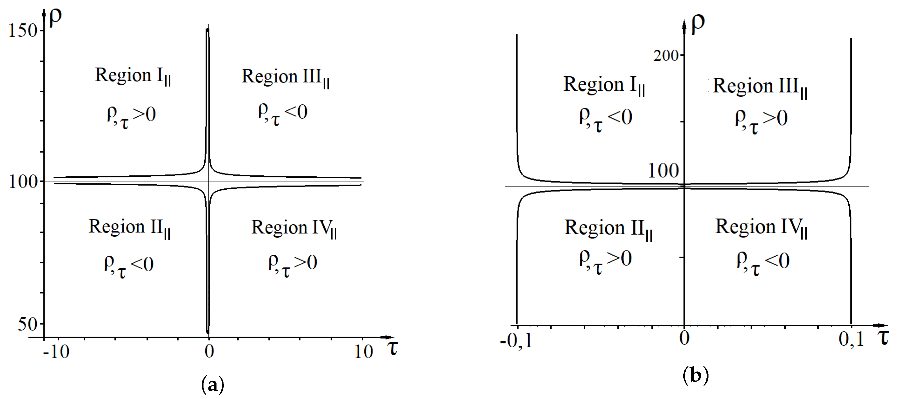
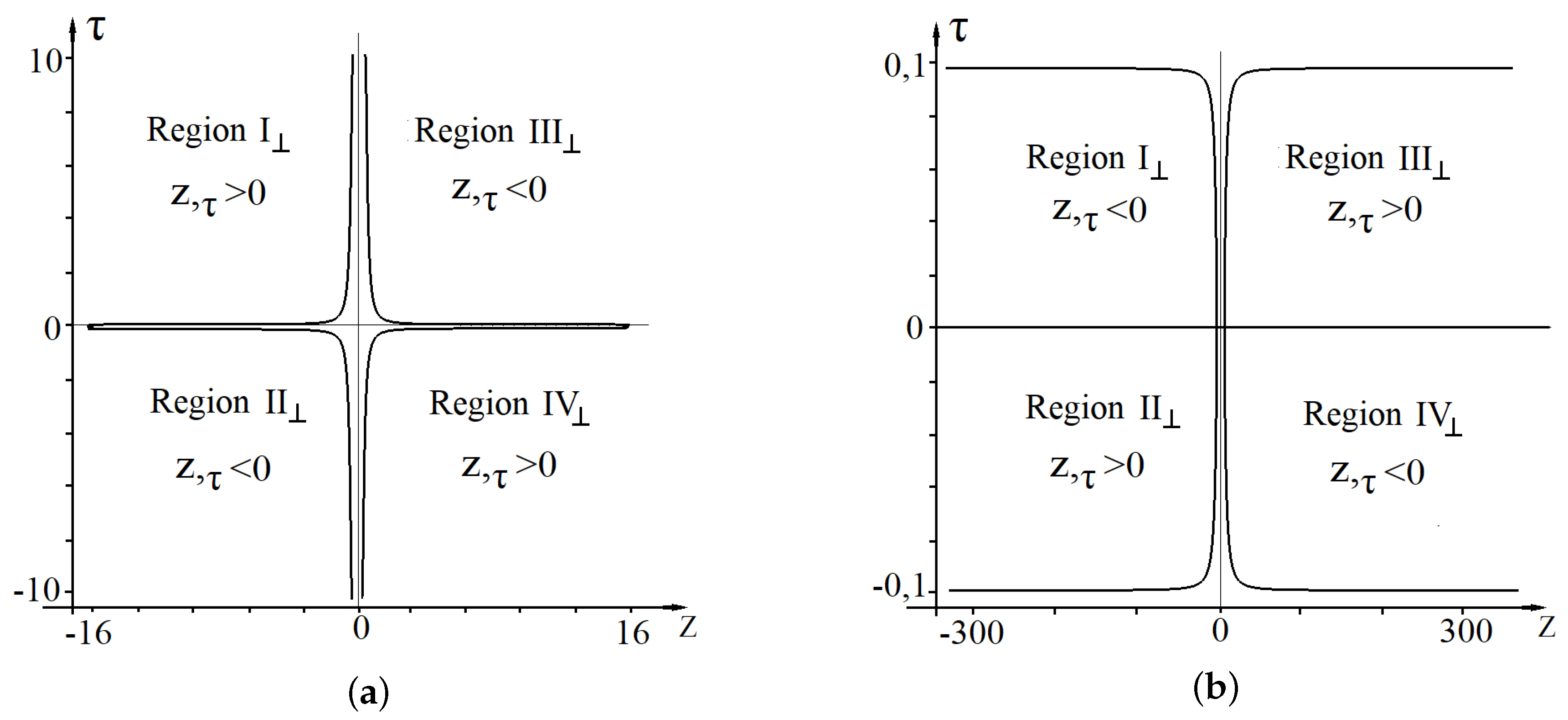
For (12) the range of the variables $q_i$ and $\rho$ depending on the sign of the derivatives of the functions ${\lambda }_{\parallel }\left(q_i\right)$ and $f_{\parallel }\left(\rho \right)$ splits into four regions [13]:

Region ${\mathbf{I}}_{\parallel }$:

$$q_i\in (-\infty ,q_i^{\prime 0}),\rho \in (R_0^{\prime },+\infty ),$$

Region ${\mathbf{II}}_{\parallel }$:

$$q_i\in (-\infty ,q_i^{\prime 0}),\rho \in [0,R_0^{\prime }),$$

Region ${\mathbf{III}}_{\parallel }$:

$$q_i\in (q_i^{\prime 0},+\infty ),\rho \in (R_0^{\prime },+\infty ),$$

Region ${\mathbf{IV}}_{\parallel }$:

$$q_i\in (q_i^{\prime 0},+\infty ),\rho \in [0,R_0^{\prime }),$$

where

$$q_i^{\prime 0}=q_i^0-{ϵ}_1^{\parallel }/{\xi }_1^{\parallel },R_0^{\prime }=R_0-{ϵ}_2^{\parallel }/{\xi }_2^{\parallel }.$$

For (4) and (12) the solution of the equations of motion of the test null string is [13]

$$t\pm z=q_i^{\prime 0}\mp \frac{1}{{\xi }_1^{\parallel }}\sqrt{{ln}^{-1}{\left(1-\frac{f_{\parallel 0}}{f_{\parallel 0}+P_{\parallel 1i}\left|\tau \right|}\right)}^{-1}},$$

(13)

$$t\mp z=-q_i^0+\frac{P_{\parallel 2i}^2}{P_{\parallel 1i}}\tau ,$$

(14)

for case ${\rho }_{,\tau }>0$

$$f_{\parallel I,IV}\left(\rho \right)=g_{\parallel }^0-P_{\parallel 2i}\left|\tau \right|,f_{\parallel II,III}\left(\rho \right)=g_{\parallel }^0+P_{\parallel 2i}\left|\tau \right|,$$

(15)

for case ${\rho }_{,\tau }<0$

$$f_{\parallel II,III}\left(\rho \right)=g_{\parallel }^0-P_{\parallel 2i}\left|\tau \right|,f_{\parallel I,IV}\left(\rho \right)=g_{\parallel }^0+P_{\parallel 2i}\left|\tau \right|,$$

(16)

where $P_{\parallel 1i}$ and $P_{\parallel 2i}$ are the initial momenta of the points of the test null string, the index on the left side of the equalities (15) and (16) shows the number of the region in which this solution is realized, $g_{\parallel }^0$ is a constant.

On the right side of the equality (13) we select the upper sign for the regions ${\mathbf{I}}_{\parallel }$ and ${\mathbf{II}}_{\parallel }$ and the lower sign for the regions ${\mathbf{III}}_{\parallel }$ and ${\mathbf{IV}}_{\parallel }$.

In the regions ${\mathbf{I}}_{\parallel }$ and ${\mathbf{II}}_{\parallel }$, the values of the parameter $\tau$ belong to the interval

$$\tau \in (-\infty ,{\tau }^{\prime }),$$

and in the regions ${\mathbf{III}}_{\parallel }$ and ${\mathbf{IV}}_{\parallel }$

$$\tau \in ({\tau }^{\prime },+\infty ),$$

where the constant ${\tau }^{\prime }$ determines the value of the parameter $\tau$ at the boundary of the regions (for $q_i=q_i^{\prime 0}$).

It can be noted that the trajectory of the test null string in the gravitational field of the source null string can be determined only in some limited area, which is called the “interaction zone”. Indeed, according to the above relations, in the whole space the parameter $\tau$ can take values that belong to the unlimited interval $(-\infty ,+\infty )$. The equalities (15) and (16) limit the possible values of the parameter $\tau$, since their left side is a limited function and the right side is linear in the parameter $\tau$. According to (13) and (14), a restriction on the values of a time-like parameter $\tau$ leads to restrictions on the values of the variables z and t for a test null string, i.e., it leads to the formation of a region beyond which the behavior of the test null string is not defined.

4. The Motion of a Test Null String in a Gravitational Field (8)

When integrating the equations of motion of a test null string for a quadratic form (8), we will be interested in the case

$${\eta }_j={\eta }_j\left(\tau \right),h_j=h_j\left(\tau \right),z=z\left(\tau \right),{\eta }_{j,\tau }>0,h_{j,\tau }>0,\theta =\theta \left(\sigma \right),$$

(17)

where $h_j=t\pm \rho$.

For the case (17), the test null string has a shape of a circle and moves “towards” (in the variable $\rho$) the null string which is the source of the gravitational field. Moreover, at each moment of time, the test null string and the source null string are coaxial and are in parallel planes.

It is important to note that the case (17) describes not only the motion of the test null string in the direction opposite to the direction of the source null string (source) (for example, a test null string radially expanding while the source null string is radially collapsing, or vice versa), but also situation where the test null string is moving along the z axis not changing its size (radius), as well as the situation where the test null string is moving in the same direction as the source null string (i.e., also radially expands or collapses), but the projections of velocities of the test null string points in the variable $\rho$ is less than the speed of light (for example, it is radially expanding or collapsing and is simultaneously moving along the z axis).

For (17) the range of the variables ${\eta }_j$ and z depending on the sign of the derivatives of the functions ${\lambda }_{\perp }\left({\eta }_j\right)$ and $f_{\perp }\left(z\right)$ splits into four regions [19,20]:

Region ${\mathbf{I}}_{\perp }$:

$$z\in (-\infty ,z_0^{\prime }),{\eta }_j\in ({\eta }_j^{\prime 0},+\infty ),$$

Region ${\mathbf{II}}_{\perp }$:

$$z\in (-\infty ,z_0^{\prime }),{\eta }_j\in (-\infty ,{\eta }_j^{\prime 0}),$$

Region ${\mathbf{III}}_{\perp }$:

$$z\in (z_0^{\prime },+\infty ),{\eta }_j\in ({\eta }_j^{\prime 0},+\infty ),$$

Region ${\mathbf{IV}}_{\perp }$:

$$z\in (z_0^{\prime },+\infty ),{\eta }_j\in (-\infty ,{\eta }_j^{\prime 0}),$$

where

$${\eta }_j^{\prime 0}={\eta }_j^0-{ϵ}_1^{\perp }/{\xi }_1^{\perp },z_0^{\prime }=z_0-{ϵ}_2^{\perp }/{\xi }_2^{\perp }.$$

For (8) and (17) the solution of the equations of motion of the test null string is [19,20]

$$t\mp \rho ={\eta }_j^{\prime 0}\mp \frac{1}{{\xi }_1^{\perp }}\sqrt{{ln}^{-1}{\left(1-\frac{f_{\perp 0}}{f_{\perp 0}+P_{\perp 1j}\left|\tau \right|}\right)}^{-1}},$$

(18)

$$t\pm \rho =-{\eta }_j^0+\frac{P_{\perp 2j}^2}{P_{\perp 1j}}\tau ,$$

(19)

for case $z_{,\tau }>0$

$$f_{\perp I,IV}\left(z\right)=g_{\perp }^0-P_{\perp 2j}\left|\tau \right|,f_{\perp II,III}\left(z\right)=g_{\perp }^0+P_{\perp 2j}\left|\tau \right|,$$

(20)

for case $z_{,\tau }<0$

$$f_{\perp II,III}\left(z\right)=g_{\perp }^0-P_{\perp 2j}\left|\tau \right|,f_{\perp I,IV}\left(z\right)=g_{\perp }^0+P_{\perp 2j}\left|\tau \right|,$$

(21)

where $P_{\perp 1j}$ and $P_{\perp 2j}$ are the initial momenta of the points of the test null string, the index on the left side of the equalities (20) and (21) shows the number of the region in which this solution is implemented, $g_{\perp }^0$ is a constant.

On the right side of the equality (18), we select the upper sign for the regions ${\mathbf{II}}_{\perp }$ and ${\mathbf{IV}}_{\perp }$ and the lower sign for the regions ${\mathbf{I}}_{\perp }$ and ${\mathbf{III}}_{\perp }$.

In the regions ${\mathbf{II}}_{\perp }$ and ${\mathbf{IV}}_{\parallel }$, the values of the parameter $\tau$ belong to the interval

$$\tau \in (-\infty ,{\tau }^{″}),$$

and in the regions ${\mathbf{I}}_{\perp }$ and ${\mathbf{III}}_{\perp }$

$$\tau \in ({\tau }^{″},+\infty ),$$

where the constant ${\tau }^{″}$ determines the value of the parameter $\tau$ at the boundary of the regions (for ${\eta }_j={\eta }_j^{\prime 0}$).

The graphs that characterize the motion of a test null string in the gravitational field of a closed null string moving along the z axis without change of the size and also in the gravitational field of a radially expanding or radially contracting closed null string clearly demonstrate a number of general regularities that can be considered as a basis for research of gravitational interaction of null strings.

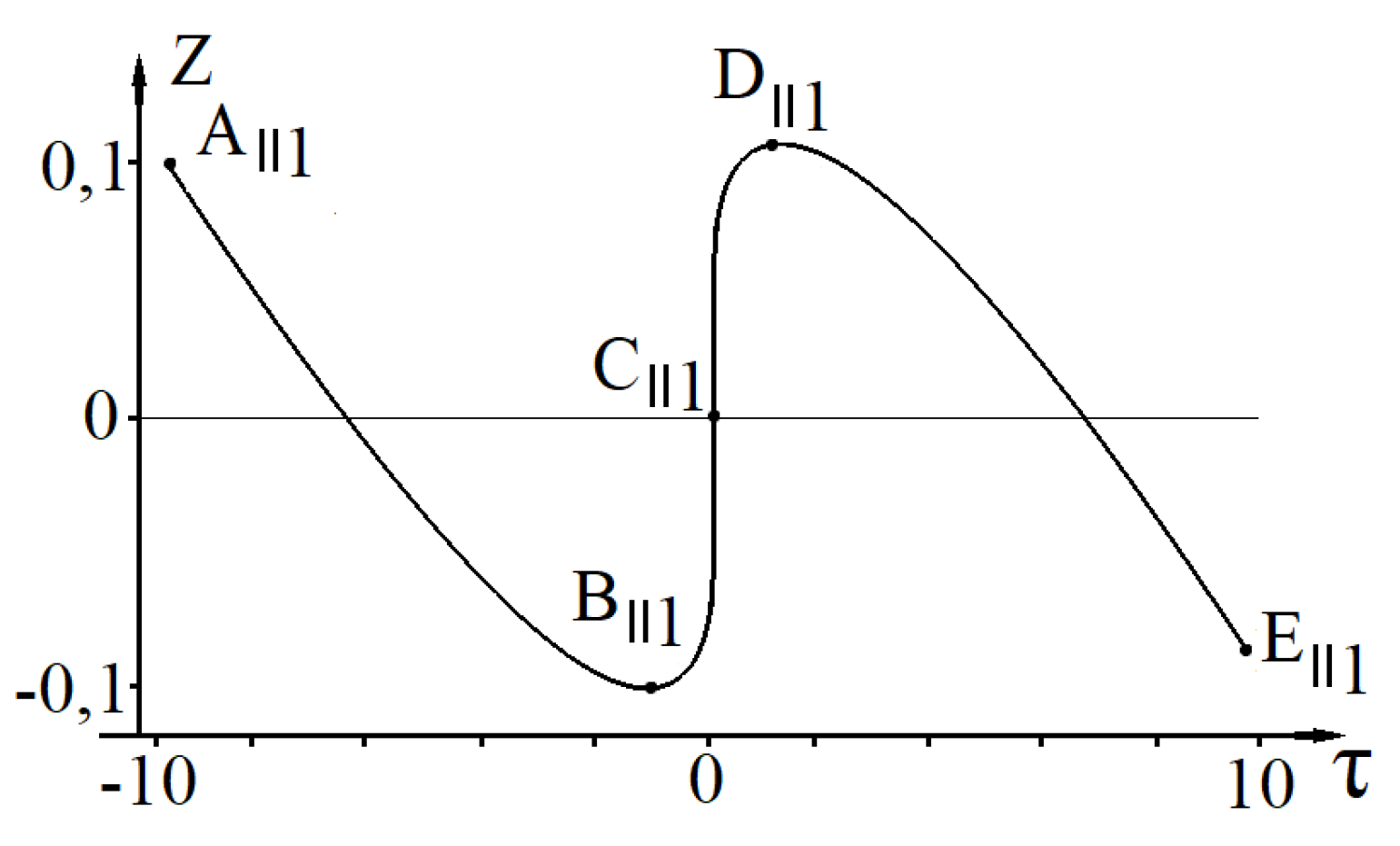
5. Graphs of the Motion of the Test Null String in a Variable Corresponding to the Direction of Motion of the Source Null String

The graphs illustrated in Figure 1, Figure 2 and Figure 3 show that the influence of the gravitational field of the source null string on the test null string in a variable, in the direction of which the source null string moves, is similar to the influence of an elastic medium.

Thus, in Figure 1 a graph of the change in the position of the test null string on the z axis in the case when the source null string moves in the negative direction of the z axis is shown. It can be seen that in the $A_{\parallel 1}$–$B_{\parallel 1}$ segment the test null string also moves in the negative direction of the z axis (we can say that the test null string is pushed out by the increasing gravitational field of the source null strings). From the provided table (

Table 1. Values of the variable z for the test null string and the source null string.

Position on the z Axis
Point	Test Null String	Source Null String
$A_{\parallel 1}$	$z=0.1$	$z=1$
$B_{\parallel 1}$	$z=-0.1$	$z=0.1$
$C_{\parallel 1}$	$z=0$	$z=0$
$D_{\parallel 1}$	$z=0.1$	$z=-0.1$
$E_{\parallel 1}$	$z=-0.1$	$z=-1$

) it can be seen that the distance in the variable z between the test null string and the source null string on the segment $A_{\parallel 1}$–$B_{\parallel 1}$ decreases.

On the segment $B_{\parallel 1}$–$D_{\parallel 1}$, the test null string moves towards the source null string, i.e., in the positive direction of the z axis. At the point $C_{\parallel 1}$, the test null string and the source null string are on the same surface ($z=0$). On the segment $D_{\parallel 1}$–$E_{\parallel 1}$, the test null string again moves in the negative direction of the z axis. However, the distance in the variable z between the test null string and the source null string in this segment is already increasing (we can say that the test null string is attracted by the decreasing gravitational field of the source null string). At the point $E_{\parallel 1}$, the test null string leaves the zone of interaction of the source null string.

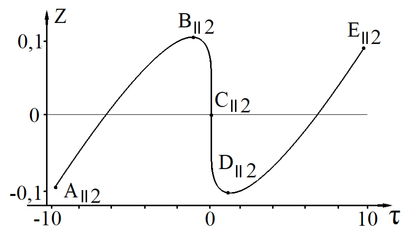
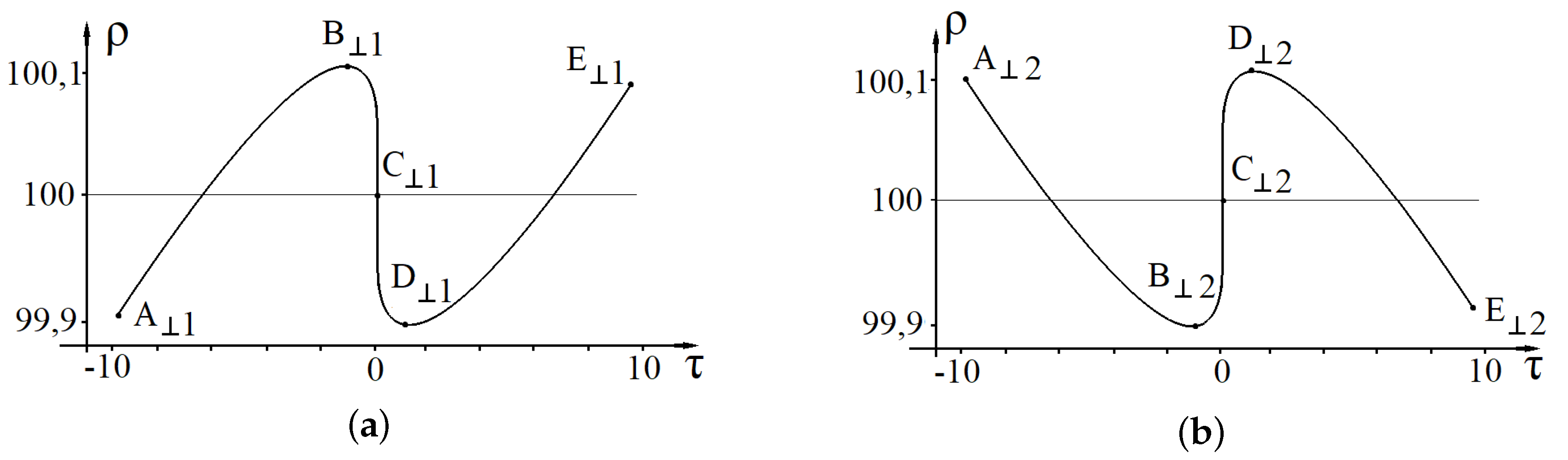
A similar “elastic” effect on the motion of a test null string in the variable z is exerted by the gravitational field of the source null string which moves in the positive direction of the z axis (Figure 2), or in the variable $\rho$ in the case of radial expansion or radial contraction of the source null string, which is shown respectively on Figure 3a,b.

6. Graphs of the Motion of the Test Null String in a Variable That Is Orthogonal to the Direction of Motion of the Source Null String

Figure 4 shows the graphs of the change in the radius of the test null string when moving in the regions ${\mathbf{I}}_{\parallel }$–${\mathbf{IV}}_{\parallel }$ in the case when the source null string, moves along the z axis without change of the radius.

You can see that each trajectory shown in Figure 4 for the corresponding region can be conventionally divided into two segments. Namely, the anomalous segment on which the test null string makes a significant displacement in a very short period of time, i.e., in this segment the test null string is strongly influenced by the gravitational field of the source null string and the segment on which this influence is weak.

This is also true for the case shown in Figure 5 which shows the graphs of the change of the position of the test null string on the z axis when it moves in the regions ${\mathbf{I}}_{\perp }$–${\mathbf{IV}}_{\perp }$ in the case when the source null string radially decreases or increases its size (radius) while being on the surface $z=z_0$.

The variables along which the anomalous sections of the trajectory of the test null string are realized correspond to the variables along which there is no motion of the null string which is the source of the gravitational field. Namely, the variable $\rho$ for the case of the motion of the test null string in the field of the closed null string of constant radius (Figure 4), and the variable z for the case of motion of the test null string in the field of the closed null string which radially expands or radially contracts orthogonally to the z axis (Figure 5).

7. Gravitational Null Strings Interaction

It can be assumed that the reason for the occurrence of anomalous segments of the trajectories of the test null string is the impossibility of taking into account the mutual influence on the movement for each of two gravitationally interacting null-strings in the solved model problem of the movement of a test null string.

However, if it is physically reasonable to assume that the speed of the null string points on the anomalous segment of the trajectory is constant and equal to the speed of light (since the null string is a null object), and the strong interaction on the anomalous segment should lead to a change in the trajectory of the source null string, then the mutual gravitational influence of interacting null strings can be taken into account.

Namely, it is possible, since on the anomalous segment of the trajectory the test null string either radially changes its size or moves along the z axis with a constant radius, and for such types of motion of the null string their gravitational properties are determined.

Then, in order to take into account the mutual gravitational influence of two null strings, we can first assume that string 1 is a source, and string 2 is a test null string. In this case, on the trajectory of string 2 there will be an anomalous segment where string 2 moves orthogonal to the direction of motion of string 1. In order to take into account the effect of string 2 on the movement of string 1, we swap strings 1 and 2 (string 2 is the source, and string 1 is test string). In other words, we will assume that string 2 moves at a constant speed (speed of light) in the anomalous segment of the trajectory and string 1 moves in the gravitational field of string 2. Such alternation on anomalous segments of the trajectory of a test null string and a source null string allows to approximately take into account the mutual influence and qualitatively construct the trajectories of motion for each of two gravitationally interacting null strings.

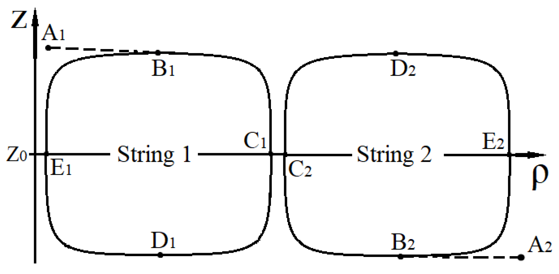
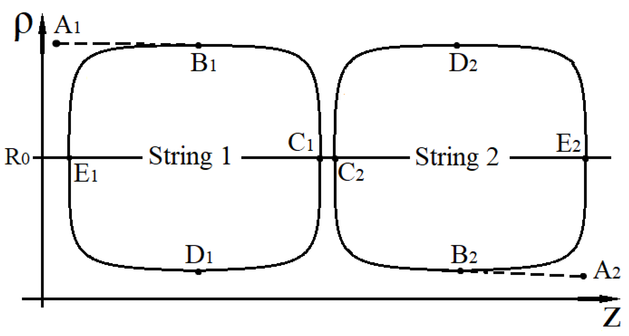
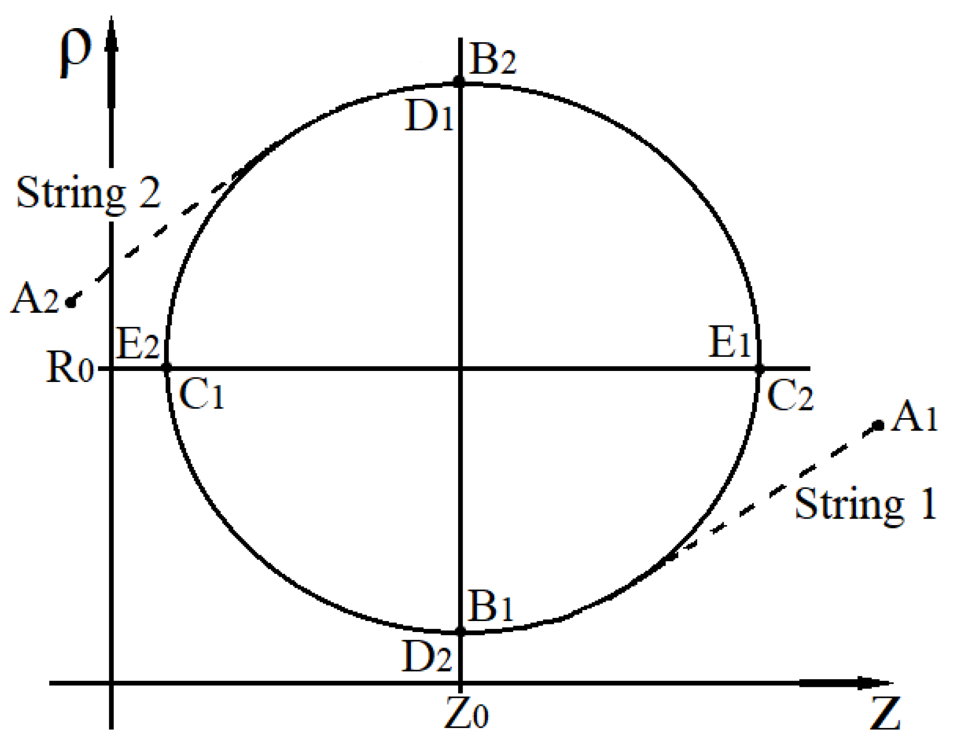
Figure 6, Figure 7 and Figure 8 qualitatively give examples of the trajectories of motion for two gravitationally interacting null strings, in which their mutual gravitational influence leads to oscillations of each null strings inside a space-limited region.

In Figure 6, Figure 7 and Figure 8 the points $A_1$ and $A_2$ fix the radius and position on the z axis, which have respectively string 1 and string 2 at the boundary of the interaction zone. The direction of motion for each null string is specified by a sequence of points: $A_l$, $B_l$, $C_l$, $D_l$, $E_l$, $B_l$, …, where the subscript l takes two values 1 and 2 and denotes the number of the null string. Points on the trajectories of two gravitationally interacting null strings, which are denoted by the same letter (regardless of indices), determine the position in space of each null string for the same value of the variable t.

For the situation shown in Figure 6 during one complete oscillation both null strings are located twice on the same surface (they meet) respectively at the points $C_l$ and $E_l$, ($l=1$; 2). The meeting surface is the surface $z=z_o$.

For the situation shown in Figure 7 during one complete oscillation both null strings are located twice on the same surface (they meet), namely, at the points $C_l$, and $E_l$, ($l=1$; 2). The meeting surface is the surface $\rho =R_o$.

For the situation shown in Figure 8 during one full oscillation both null strings are located on the same surface four times. The first time both null strings meet on the surface $z=z_o$ (points $B_1$ and $B_2$), the second time they meet on the surface $\rho =R_o$ (points $C_1$ and $C_2$), the third time they meet on the surface $z=z_o$ (points $D_1$ and $D_2$), the fourth time they meet on the surface $\rho =R_o$ (points $E_1$ and $E_2$). Thus, for the situation shown in Figure 8, the meeting surfaces alternate.

Each of the cases of motion of two null strings shown in Figure 6, Figure 7 and Figure 8 leads to the formation of a region limited in space, within which oscillations of gravitationally interacting null strings occur. These regions can be considered as particles localized in space with an effective nonzero rest mass.

The “lifetime” of such particles should depend on external conditions. So, it is obvious that for each solitary pair of gravitationally interacting null strings shown in Figure 6, Figure 7 and Figure 8 the “lifetime” is not limited. However, in the case of a gas of null strings, gravitational interaction with external null strings, depending on the situation, can lead to both the long-term existence of such particles and their possible rapid destruction.

Long-term existence (“lifetime”) of such particles is possible if they are combined into more complex structures. The possibility of such a combination depends on the direction of motion of the null strings that form the particles.

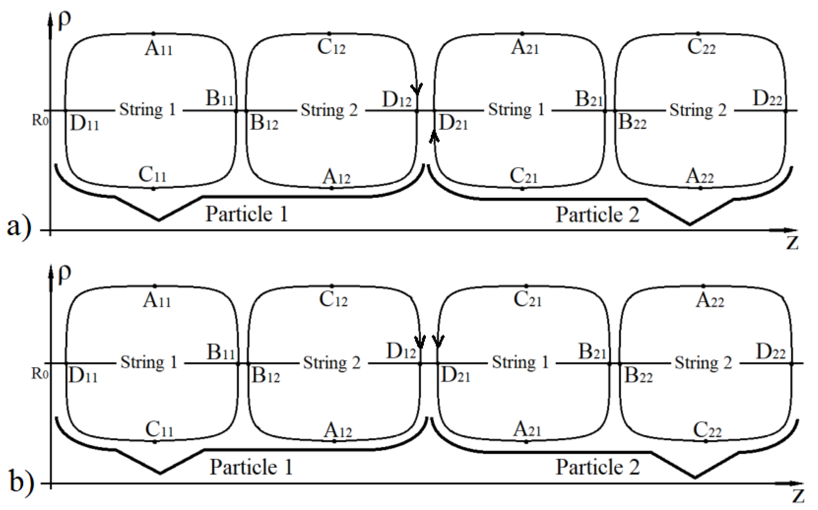
Thus, Figure 9 shows two cases of the location of two pairs of interacting null strings (“particle 1” and “particle 2”). The direction of motion for each null string is specified by a sequence of points: $A_{lk}$, $B_{lk}$, $C_{lk}$, $D_{lk}$, $A_{lk}$, …, where the first index corresponds to the number of the particle and the second index corresponds to the number of the null string. Points on the trajectories of motion of null strings, which are denoted by the same letter (regardless of indices), determine the position in space of each null string for the same time value.

For the case shown in Figure 9b the trajectories of null strings belonging to “particle 1” and “particle 2” violate the condition of intersection of the meeting surface, and therefore this case of location is not realized. It can be seen that the case shown in Figure 9b differs from the case shown in Figure 9a only in the position of the second pair of interacting null strings. Moreover, changing in Figure 9b the spatial orientation of “particle 2” along the z axis to the opposite one, we obtain the case of the arrangement of particles shown in Figure 9a.

To characterize the direction of motion of null strings that form a “particle”, one can define a vector orthogonal to the plane of location of null strings that form the particle. Moreover, for the possibility of combining interacting null strings into some complex formations (in the given example it is a “one-dimensional” object that can be roughly called a “thread”) the directions of the vectors (at least locally) must coincide.

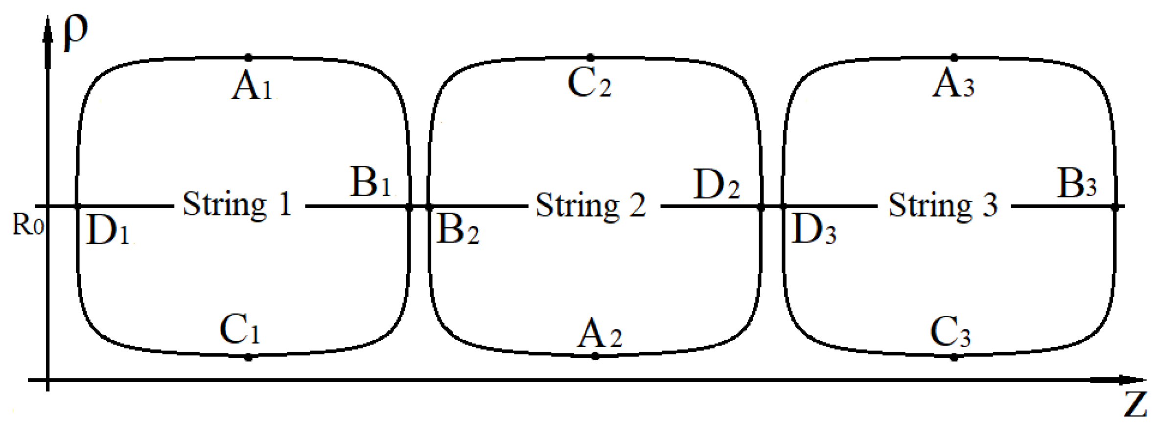
It can be noted that the process of generation of complex formations consisting of interacting null strings is not necessarily associated with the union of already formed “particles” (pairs of gravitationally interacting null strings), for example, the situation shown in Figure 10 is possible, in which three null strings are gravitationally united.

8. Discussion

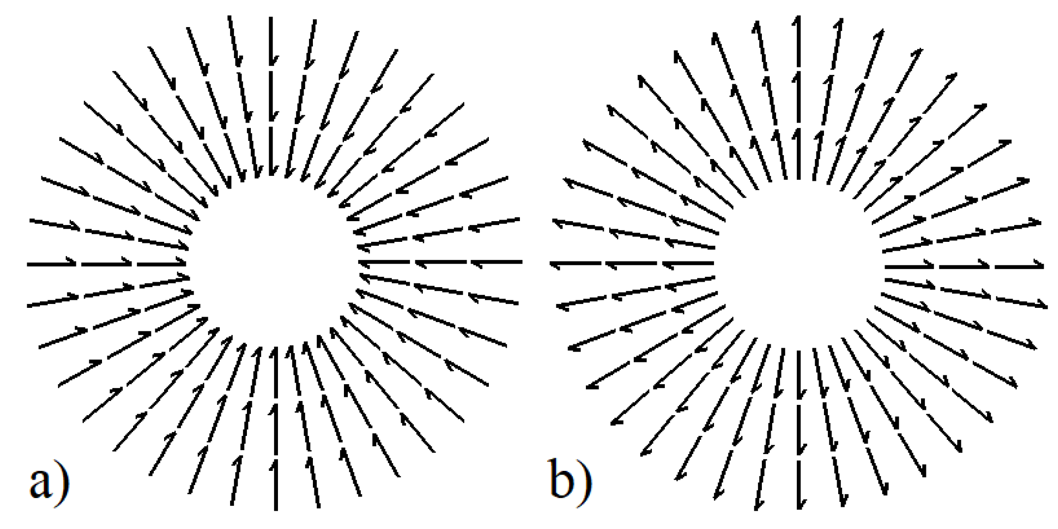
Formed “threads” can be part of more complex spatial structures. The most interesting is the possibility of combining the “threads” into spherically symmetric formations (domains). With such a union, null strings belonging to neighboring “threads” are located on spherical surfaces (form layers of the domain), and the “threads” themselves are located orthogonal to the layers, i.e., are located at the radii of a spherically symmetric domain. Figure 11 schematically shows two possibilities of such a combination. Each vector in Figure 11 corresponds to a null string (the vector characterizes the direction of motion of a gravitationally interacting null string that forms a “thread”). The plane of location of null strings forming the domain is orthogonal to the direction of the corresponding vector.

Being in a gas of null strings, such “macro” objects cannot have a completely formed (static) structure. The presence of external (“free”) null strings, other “macro” objects in the gas, the possible movement of “macro” objects relatively to each other, the existence of a interaction zone for each null string, being outside which the null strings do not experience the gravitational influence of each other, should lead to a random (dynamic) change in the number of null strings gravitationally belonging to a given “macro” object, and, as a consequence, to a random (dynamic) change in the spatial form of the “macro” object (domain).

In such a situation, it is impossible to talk about symmetry, the number of structural elements, the shape of a “macro” object at a fixed moment of time. But by averaging over time various spatial forms (distributions) of “macro” objects in a gas of null strings, one can introduce the concepts of “substance” and “field”. Averaged over a long period of time “macro” objects form “substance” and structures associated with “macro” objects, the “lifetime” of which is shorter, form a “field”. With a decrease in the observation time “particles” will appear in the “field”, which can be interpreted as carriers of interaction. Moreover, the shorter the observation time, the more quantitatively and spatially more diverse the structures that form the “field”.

The question of the interaction of various “macro” objects, and, as a consequence, the question of the motion of “macro” objects respectively to each other, should be related to the question of the influence of the external “ordered” distribution of null strings on the motion of a solitary null strings.

In the papers [19,20] the simplest (model) problems of the motion of a test null string in the gravitational field of a layered domain of null strings (multi-string system) were investigated. In these works, it was shown that, depending on the ratio of the parameters characterizing the test null string and the null string domain, the region within which the test null string (“particle”) oscillates is shifted (drifted) in space.

Such coordinated movements of null strings, which are constituent elements of spatial structures that form the field of interaction between “macro” objects, can cause the appearance of “tensions” (“rigidity”) of such structures, and as a consequence, lead to the movement of “macro” objects (field sources).

The proposed qualitative method for taking into account the mutual influence of gravitationally interacting null strings cannot help in determination of the characteristics of the interaction between “macro” objects. In such a situation, only some indirect reasoning is possible. Thus, one can argue about the possibility of the formation of “threads” or other extended structures of the interaction field, which “connect” (spatially) “macro” objects that have different structures (different directions of vectors characterizing the motion of null strings forming a “macro” object). For example, it can be the “macro” objects shown in Figure 11a,b. It can also be argued that it is impossible to form extended structures that spatially connect two “macro” objects with the same structure. For example, both “macro” objects have the structure shown in Figure 11a or the structure shown in Figure 11b.

The presence of “tension” (“rigidity”) in admissible extended structures of the interaction field which “connect” “macro” objects of various structures can indirectly indicate the possibility of realization of the “attraction” of such “ macro ” objects. The inadmissibility of the formation of extended structures of the interaction field “connecting” the “macro” objects of the same structure can indirectly speak of the possibility of realization of the “repulsion” of such “macro” objects.

It is interesting to note that since the solutions (4) and (8) are obtained for the null string model in the form of a thin tube of a massless scalar field, then, in essence, the processes in a null string gas are processes in a gas of thin tubes of a massless scalar field. The gravitational interaction between the elements of this field leads to the appearance of a “mass” in the scalar field (primary particles with a nonzero rest mass are “formed”). Further gravitational interaction of primary particles in the gas leads to the formation of “stable” in time “macro” objects, the interaction between which, in fact, remaining gravitational, leads to the appearance of polarization waves of the vector field associated with a change (rearrangement) of structures, forming the field of interaction. While propagating, such waves affect the formation of structures of the interaction field between “macro” objects, i.e., affect the interaction between “macro” objects (sources).