Article

Quark Stars in Massive Brans–Dicke Gravity with Tolman–Kuchowicz Spacetime

Department of Mathematics, University of the Punjab, Quaid-e-Azam Campus, Lahore 54590, Pakistan
*
Author to whom correspondence should be addressed.
Universe 2020, 6(8), 124; https://doi.org/10.3390/universe6080124
Submission received: 14 July 2020 / Revised: 7 August 2020 / Accepted: 8 August 2020 / Published: 13 August 2020

Abstract

:
In this paper, we construct anisotropic model representing salient features of strange stars in the framework of massive Brans–Dicke gravity. We formulate the field equations for Tolman–Kuchowicz ansatz by incorporating the MIT bag model. Junction conditions are applied on the boundary of the stellar model to evaluate the unknown constants in terms of mass and radius of the star. The radius of the strange star candidate PSR J1614-2230 is predicted by assuming maximum anisotropy at the surface of the star for different values of the coupling parameter, mass of the scalar field and bag constant. We examine various properties as well as the viability and stability of the anisotropic sphere. We conclude that the astrophysical model agrees with the essential criteria of a physically realistic model for higher values of the coupling parameter as well as mass of the scalar field.

1. Introduction

Self-gravitating systems such as stellar and galactic structures constitute a major part of the visible universe. The study of the evolution of these systems plays a crucial role in revealing various hidden aspects (composition, evolution, age) of the cosmos. One of the important evolutionary phases of a star is the process of gravitational collapse near its death which leads to the formation of dense compact objects. The neutron star is one of the intriguing outcomes of collapse with a dense core of about 1 M to 3 M ( M is the solar mass). The degeneracy pressure of neutrons resists the strong inward gravitational pull and halts the process of collapse. Since radiation emitted by neutron stars is less as compared to other cosmic objects, therefore, they are difficult to detect. Baade and Zwicky [1] predicted the existence of neutron stars in 1934. However, the first rapidly rotating pulsar was discovered in 1967 which pulsated at a regular interval of 1.37 s [2].
According to the Tolman–Oppenheimer–Volkoff limit, a stable neutron star must have a mass of at most 3 M . If the mass exceeds this limit, it is hypothesized that neutrons lose their individuality under extreme pressure and breakdown into quarks. Quark matter can exist in the universe in two scenarios: the transition phase of quark-hadron in the initial era of the cosmos or the evolution of neutron stars into strange quark stars [3]. A quark star is smaller in size but ultra-dense as compared to the neutron star. However, increased pressure in its core stops quark stars from collapsing into black holes. It has been proposed that the amount of energy emitted in extremely luminous supernovae (observed once in every thousand supernovae) can be explained with the help of stable strange quark stars [4,5]. Moreover, estimates of radii of some stellar objects (LMC X-4, 4U 1820-30, Her X-1, etc.) suggest that their structure and characteristics may be similar to that of strange quark stars.
Interactions among tightly packed nuclear matter generate anisotropy in a system with high density [6]. Bowers and Liang proposed that extreme density at the core of celestial structures (like compact stars) makes them highly anisotropic in nature [7]. Anisotropy may be the result of different physical processes such as the presence of superfluid, phase transition or magnetic field [8,9,10]. Researchers have investigated salient properties of cosmic objects by introducing anisotropic pressure in matter source. Herrera and Santos [11] studied different aspects of anisotropic self-gravitating objects and identified the causes of local anisotropy. Harko and Mak [12] considered the anisotropy factor to obtain static interior solutions of relativistic objects. Hossein et al. [13] included cosmological constant to explore the stability of anisotropic systems. Viable solutions were derived for spherical systems in equilibrium by Paul and Deb [14]. Recently, Maurya et al. [15] presented a class of physically realistic solutions representing static anisotropic stars by incorporating Buchdahl’s ansatz.
Equation of state (EoS) relating different physical properties of the matter distribution is often introduced in the modeling of an astrophysical configuration to describe the realistic scenario within the stellar structure. An agreement on the most suitable EoS representing quark stars has not been achieved. Witten [3] conjectured that the quark star is composed of strange quark matter (SQM) containing strange, up and down quarks. The confined hadrons can exist in their true ground state in a hypothetical quark star [16,17]. As the EoS for neutron star does not accurately describe the compact objects like SAX J 1808.4-3658, Her X-1, PSR J1614-2230, etc. therefore, the MIT bag model (SQM EoS) [18] is chosen as the most suitable representative of quark stars. Moreover, recent statistics obtained from the collision of binary neutron stars (GW170817 [19] and GW190425 [20]) have provided an estimation of masses of neutron stars as well as strange stars which support the assumption of MIT bag model as an EoS for quark stars.
The difference between the energy density of true and false vacuums is incorporated in the MIT bag EoS through a bag constant ( B ). The bag constant lies within the range 58.9–91.5 MeV/fm 3 [21] for massless strange quarks whereas the range of B for massive quarks is of 56–78 MeV/fm 3 [22]. However, researchers have also considered larger values of B . Xu et al. [23] found that the cosmic body LMXB EXO 0748-676 can serve as a strange star candidate for two values of B . Further, the experimental data of RHIC and CERN-SPS also allow higher values of the bag constant [24,25]. The MIT bag model has been employed in literature to discuss the structure and characteristics of quark stars [26,27,28]. Rahaman et al. [29] calculated the mass of a star of radius 9.9   km using MIT bag model. Bhar [30] employed Krori and Barura ansatz to study a hybrid star made of quark matter. Anisotropic quark star models have been constructed in the presence of charge as well [31,32,33]. Deb et al. [34] examined different physical properties of strange stars for B = 83 MeV/fm 3 , 100 MeV/fm 3 , 120 MeV/fm 3 . Bhar [35] investigated the viability as well as the stability of quark models through the condition of embedding class-one.
Dirac’s hypothesis in 1937 suggested that the gravitational constant (G) varies with respect to cosmic time [36,37]. In 1961, Brans and Dicke [38] incorporated the dynamical gravitational constant in terms of a massless scalar field ( ϕ ) and modified general relativity (GR). Brans–Dicke (BD) theory, a scalar-tensor theory, is based on the Machian principle. The matter distribution is coupled to the dynamical scalar field through a tunable coupling parameter ( ω B D ) in Jordan frame. The weak-field tests put a lower limit on the coupling parameter as ω B D > 40 , 000 [39]. However, as higher values of scalar field support rapid expansion of the cosmos, the inflationary era is explained for small values of the coupling parameter [40]. The issue is resolved through a potential function that allows a massive scalar field ( Ψ ). Thus, the BD gravity is modified to Massive BD (MBD) theory in which the mass of scalar field ( m Ψ ) provides a finite range of the scalar field in terms of its compton wavelength ( λ Ψ ). The constraints on the coupling parameter due to solar system observations vanish for m Ψ 2 × 10 25 GeV and ω B D > 3 2 [41].
Various astrophysical phenomena have been discussed in scalar-tensor gravity. Sotani [42] discussed deviations from GR while studying neutron stars in the presence of a massless scalar field. Silva et al. [43] analyzed the inertia of anisotropic neutron stars. The effects of a massive scalar field on rapidly rotating neutron stars were studied by Doneva and Yazadjiev [44] and it was verified that deviations from GR increase for larger inertia. This work was extended by employing a self-interacting potential to examine the structure of slowly rotating neutron stars [45]. Researchers have constructed different models for quark stars in modified theories of gravity as well [46,47,48,49]. Recently, we have used the condition of embedding class-one to generate anisotropic model for quark stars in the background of MBD gravity [50].
In this paper, we formulate anisotropic model obeying MIT bag model with Tolman–Kuchowicz (TK) ansatz in the context of MBD theory. We further check the viability and stability of the resulting stellar model. The matter variables obeying the MIT bag model are obtained from MBD field equations in Section 2. The necessary matching conditions on the boundary of the model are applied in Section 3. In Section 4, we examine various physical features, viability and stability of the anisotropic solution. The results are summarized in the last section.

2. Massive Brans–Dicke Theory and Matter Variables

The action of MBD gravity in Jordan frame with G 0 = 1 is defined as
S = g ( R Ψ ω B D Ψ γ γ Ψ V ( Ψ ) + L m ) d 4 x ,
where g = | g γ δ | , R is the Ricci scalar and L m represents the matter lagrangian. The MBD gravity can also be discussed in Einstein frame of reference. The conformal transformations g ^ γ δ = A 2 ( Ψ ) g γ δ and Ψ = A 2 ( Ψ ^ ) yield metric ( g ^ γ δ ) and scalar field ( Ψ ^ ) for Einstein frame. The field and evolution equations are respectively, given as
G γ δ = 1 Ψ [ T γ δ ( m ) + T γ δ Ψ ] = 1 Ψ [ T γ δ ( m ) + Ψ , γ ; δ g γ δ Ψ + ω B D Ψ ( Ψ , γ Ψ , δ g γ δ Ψ , μ Ψ , μ 2 ) V ( Ψ ) g μ ν 2 ] ,
Ψ = T ( m ) 3 + 2 ω B D + 1 3 + 2 ω B D ( Ψ d V ( Ψ ) d Ψ 2 V ( Ψ ) ) ,
where the matter source is described by the energy-momentum tensor T γ δ ( m ) and T ( m ) = T γ γ ( m ) . Moreover, □ indicates the d’Alembertian operator.
We consider a static sphere represented by the following line element
d s 2 = e ν ( r ) d t 2 e λ ( r ) d r 2 r 2 ( d θ 2 + sin 2 θ d ϕ 2 ) .
The relativistic motion of particles in compact objects leads to a random distribution throughout the interior region. Consequently, compact stellar structures are characterized by variable energy density and anisotropic pressure. Therefore, we employ the energy-momentum tensor specifying the anisotropic interior in terms of density ( ρ ), radial ( p r ) and tangential ( p ) pressures as follows
T γ δ ( m ) = ( ρ + p ) U γ U δ p g γ δ + ( p r p ) S γ S δ ,
where U γ = ( e ν 2 , 0 , 0 , 0 ) is the 4-velocity and S γ = ( 0 , e λ 2 , 0 , 0 ) . Using Equations (2)–(5), the field equations are obtained as
1 r 2 1 r 2 λ r e λ = 1 Ψ ( ρ + e λ ( Ψ + ( 2 r λ 2 ) Ψ + ω B D 2 Ψ × Ψ 2 e λ V ( Ψ ) 2 ) ) ,
1 r 2 + e λ 1 r 2 + ν r = 1 Ψ ( p r e λ ( 2 r + ν 2 Ψ ω B D 2 Ψ Ψ 2 e λ V ( Ψ ) 2 ) ) ,
e λ 4 2 ν + ν 2 λ ν + 2 ν λ r = 1 Ψ ( p e λ ( Ψ + 1 r λ 2 + ν 2 Ψ + ω B D 2 Ψ Ψ 2 e λ V ( Ψ ) 2 ) ) ,
where denotes differentiation with respect to r. The evolution Equation (3) becomes
Ψ = e λ 2 r λ 2 + ν 2 Ψ ( r ) + Ψ ( r ) , = 1 3 + 2 ω B D g γ δ T γ δ + Ψ d V ( Ψ ) d Ψ 2 V ( Ψ ) .
Extreme temperature and pressure at the core of a neutron star may transform it into a quark star composed of up strange ( s ) , up ( u ) and down ( d ) flavors. We assume that the MIT bag model governs the state determinants (density and pressure) of these relativistic stars. It is further assumed that non-interacting and massless quarks occupy the interior of the configuration. The MIT bag model defines the individual quark pressure ( p f ) as
p r = f p f B , f = u , d , s .
The total external bag pressure (or bag constant) balances the individual pressure. The deconfined quarks within the bag model have the following energy density
ρ = f ρ f + B ,
where the density of a flavor ( ρ f ) is related to the corresponding pressure as ρ f 3 = p f . Thus, Equations (10) and (11) are combined to formulate the following EoS of MIT bag model
p r = 1 3 ( ρ 4 B ) .
The metric potentials ν ( r ) = B r 2 + 2 ln F and λ ( r ) = ln ( 1 + a r 2 + b r 4 ) ( a , b , B and F are constants) define the Tolman–Kuchowicz (TK) spacetime [51,52]. Salient features of compact objects have been investigated by employing the TK metric in GR as well as modified theories of gravity [53,54,55]. The field Equations (6)–(8) are rewritten in terms of TK metric functions as
ρ = 1 2 r Ψ a r 2 + b r 4 + 1 2 2 Ψ 2 a 2 r 3 + a r 2 b r 4 + 3 + b r 3 b r 4 + 5 + r Ψ V ( Ψ ) a r 2 + b r 4 + 1 2 r ω B D a r 2 + b r 4 + 1 Ψ 2 2 Ψ r a r 2 + b r 4 + 1 Ψ ( r ) + a r 2 + 2 Ψ ,
p r = 1 4 Ψ a r 2 + b r 4 + 1 2 Ψ r Ψ a B r 2 + a + b B r 4 + 2 b r 2 + B a r 2 + b r 4 + 1 Ψ + 2 Ψ 2 a B r 2 + a + b B r 4 + 2 b r 2 + B ω B D a r 2 + b r 4 + 1 Ψ 2 B ,
p = 1 4 r Ψ a r 2 + b r 4 + 1 2 2 r Ψ 2 2 a 2 r 2 + a 4 b r 4 + 2 B 2 r 4 B r 2 + 1 + 2 b 2 r 6 + 2 B 2 b r 6 + r 2 3 b B r 4 + B + Ψ Ψ a r 2 B r 2 7 + b B r 6 10 b r 4 + B r 2 4 r a r 2 + b r 4 + 1 4 B a r 2 + b r 4 + 1 3 Ψ + 3 r ω B D a r 2 + b r 4 + 1 Ψ 2 .
In this study, we choose V ( Ψ ) = 1 2 m Ψ 2 Ψ 2 , where m Ψ denotes the mass of the scalar field. This form of potential function has been used to study neutron stars [44,56].

Junction Conditions

The constants ( a , b , B , F ) completely specify the solution in Equations (13)–(15) In order to evaluate these constants, we apply constraints at the hypersurface ( Σ : r = R ) which ensure a smooth junction between interior and exterior geometries. The Schwarzschild spacetime describes the external vacuum as
d s 2 = ( 1 2 M r ) d t 2 1 ( 1 2 M r ) d r 2 r 2 ( d θ 2 + sin 2 θ d ϕ 2 ) ,
where M is the mass. Using the procedure in [57], the scalar field associated with the external Schwarzschild metric is obtained as Ψ = e ( 1 2 M r ) . The matching at the boundary surface ( h = r R = 0 ) is continuous when the following conditions are satisfied
( d s 2 ) Σ = ( d s + 2 ) Σ , ( K i j ) Σ = ( K i j + ) Σ ,
( Ψ ( r ) ) Σ = ( Ψ ( r ) + ) Σ , ( Ψ ( r ) ) Σ = ( Ψ ( r ) + ) Σ .
Here K i j is curvature whereas interior and exterior spacetimes are represented by subscripts − and +, respectively. The metric defining the hypersurface is written as
d s 2 = d T 2 R 2 ( d θ 2 + sin 2 θ d ϕ 2 ) ,
where T represents the proper time on Σ . The curvature is given by
K i j ± = 2 z ± γ η i η j n γ ± Γ δ μ γ z ± δ η i z ± μ η j n γ ± ,
where η i are the coordinates defined on Σ . The normal ( n γ ± ) to the boundary is defined as
n γ ± = ± d h d z γ | g δ μ d h d z δ d h d z μ | 1 2 ,
with n γ n γ = 1 . Here z ± γ are the coordinates of internal/external regions. The unit normal vectors turn out to be
n γ = ( 0 , e λ 2 , 0 , 0 ) , n γ + = ( 0 , ( r 2 M r ) 1 2 , 0 , 0 ) .
Comparing the spacetimes defined by metrics (4) and (16) with (19), it follows that
( d t d τ ) Σ = ( e ν 2 ) Σ = ( ( 1 2 M r ) 1 2 ) Σ , ( r ) Σ = R .
Moreover, the non-zero components of curvature are evaluated as
K 00 = [ ν e λ 2 2 ] Σ , K 22 = sin 2 ( θ ) K 33 = [ e λ 2 r ] Σ , K 00 + = [ ( 1 2 M r ) 1 2 M r 2 ] Σ , K 22 + = sin 2 ( θ ) K 33 + = [ ( 1 2 M r ) 1 2 r ] Σ .
Employing the matching conditions on the hypersurface yields
e ν ( R ) = 2 M + R R , e λ ( R ) = 2 M + R R , ν ( R ) = 2 M ( 2 M + R ) R .
The O’Brien and Synge [58] junction conditions (equivalent to the continuity of the second fundamental form) are given as ( G γ δ r δ ) Σ = 0 , where r γ is a unit radial vector. Using this condition in the field equations implies zero radial pressure at the hypersurface. The constants appearing in the TK metric are determined in terms of mass and radius through Equation (21) and p r ( R ) = 0 as
a = 24 M 3 M 2 R ( ω B D + 34 ) 4 R 5 B 1 2 M R + 12 M R 2 R 2 ( R 2 M ) 2 ( 2 R 3 M ) ,
b = 12 M 3 + M 2 R ( ω B D + 20 ) + 4 R 5 B 1 2 M R 8 M R 2 R 4 ( R 2 M ) 2 ( 2 R 3 M ) ,
B = M R 2 ( R 2 M ) ,
F = e ( 2 M R ) ln R 2 M R + M 4 M 2 R .

3. Physical Features of Compact Stars

In this section, we analyze the influence of the massive scalar field on the physical structure of strange stars through viability and stability constraints. In the present work, the numerical solutions have been obtained by considering B = 60 MeV/fm 3 , 83 MeV/fm 3 . These values are within the allowed limits [29]. Moreover, as per the results of Gravity Probe B experiment, all values of m Ψ > 10 4 (in dimensionless units) are admissible [41,44]. Thus, we solve the wave equation numerically for m Ψ = 0.001 , 0.3 and ω B D = 5 , 8 , 10 by imposing the initial conditions Ψ ( 0 ) = Ψ c = constant and Ψ ( 0 ) = 0 . The constant Ψ c corresponding to the chosen values of the parameters B , ω B D and m Ψ are presented in Table 1 and Table 2. The quantities with subscripts s and c are derived at the surface and center of the star, respectively. The results are displayed graphically for PSR J1614-2230 ( M = 1.97 ± 0.04 M ) [59].
Literature survey reveals that anisotropy vanishes at r = 0 and then increases to attain a maximum value at the surface of the compact star [12,13,60]. Deb et al. [34] evaluated the extremum of anisotropy at the boundary and showed that for a viable and stable spherical structure anisotropy must be maximum at r = R . Adopting the procedure in [34], we predict radius of the strange star candidate PSR J1614-2230 by maximizing anisotropy at the boundary. The metric potentials must be well-behaved and positive throughout the interior region to ensure a singularity-free geometry [61]. As shown in Figure 1, the TK metric functions are monotonically increasing as well as regular functions of the radial coordinate. Energy density and pressure play a dominant role in determining the behavior of extremely dense strange stars. The matter variables must be positive and decrease monotonically towards the surface of the star. Figure 2 and Figure 3 show that the state determinants are maximum at the center and decrease away from it for the considered values of m Ψ , coupling parameter and bag constant.
The presence of radial/transverse pressure leads to anisotropy ( Δ = p p r ) within the system. The anisotropy is negative when p r > p and positive otherwise. Moreover, particles are tightly packed together in dense celestial objects which limits the particles’ movement in the radial direction. Consequently, the radial force or pressure is less than the tangential force leading to positive anisotropy. Thus, the positive anisotropy generates an outward repulsive force increasing the stability and compactness of the star. The anisotropy of the current setup, displayed in Figure 4, is calculated through Equations (14), (15) and (22)–(25). The anisotropy is positive throughout the stellar region for the considered values of m Ψ , ω B D and B .

3.1. Energy Conditions

The anisotropic configuration is physically viable if it complies with four constraints, i.e., null (NEC), weak (WEC), strong (SEC) and dominant (DEC). In the background of MBD gravity, these conditions are stated in terms of following inequalities [62].
NEC : ρ 0 , WEC : ρ + p r 0 , ρ + p 0 , SEC : ρ + p r + 2 p 0 , DEC : ρ p r 0 , ρ p 0 .
The positive trend of state determinants presented in Figure 2 and Figure 3 readily satisfies the first three inequalities. The plots of DEC in Figure 5 show that DEC is violated near the boundary of the surface for m Ψ = 0.001 . However, the setup corresponding to m Ψ = 0.3 satisfies the DEC except for ω B D = 5 as shown in Figure 6. The critical values of m Ψ for which the stellar model becomes viable are mentioned in Table 3.

3.2. Effective Mass, Compactness and Redshift

Gravitational mass (m) is one of the key features that determine the structure and compactness of stellar objects. The mass of a spherical celestial object (measured using Kepler’s law when a satellite orbits the star) is evaluated as
m = 1 2 0 r ρ r 2 d r .
The mass of the anisotropic stellar model is obtained by numerically solving the above equation along with the wave equation under the condition m ( 0 ) = 0 . The size and mass of a cosmic body provide a measure of its compactness ( μ ( r ) = m r ). Buchdal [63] proposed that a compact object is stable if μ ( r ) < 4 9 . The value of the compactness function at the surface of the star is shown in Table 4 for m Ψ = 0.001 and m Ψ = 0.3 . In both cases, the compactness parameter increases corresponding to an increase in m Ψ , ω B D or B . Moreover, it attains values less than 4 9 . Under the influence of a star’s gravitational field, the electromagnetic radiation loses some of the energy resulting in an increase in its wavelength, i.e., the radiation is redshifted. The effect of the gravitational force is measured through a redshift parameter defined as
Z = 1 1 2 u ( r ) 1 .
For an anisotropic source, the redshift must not exceed the value 5.211 [64]. The redshift parameter obeys the limit proposed in [64] (refer to Table 4).

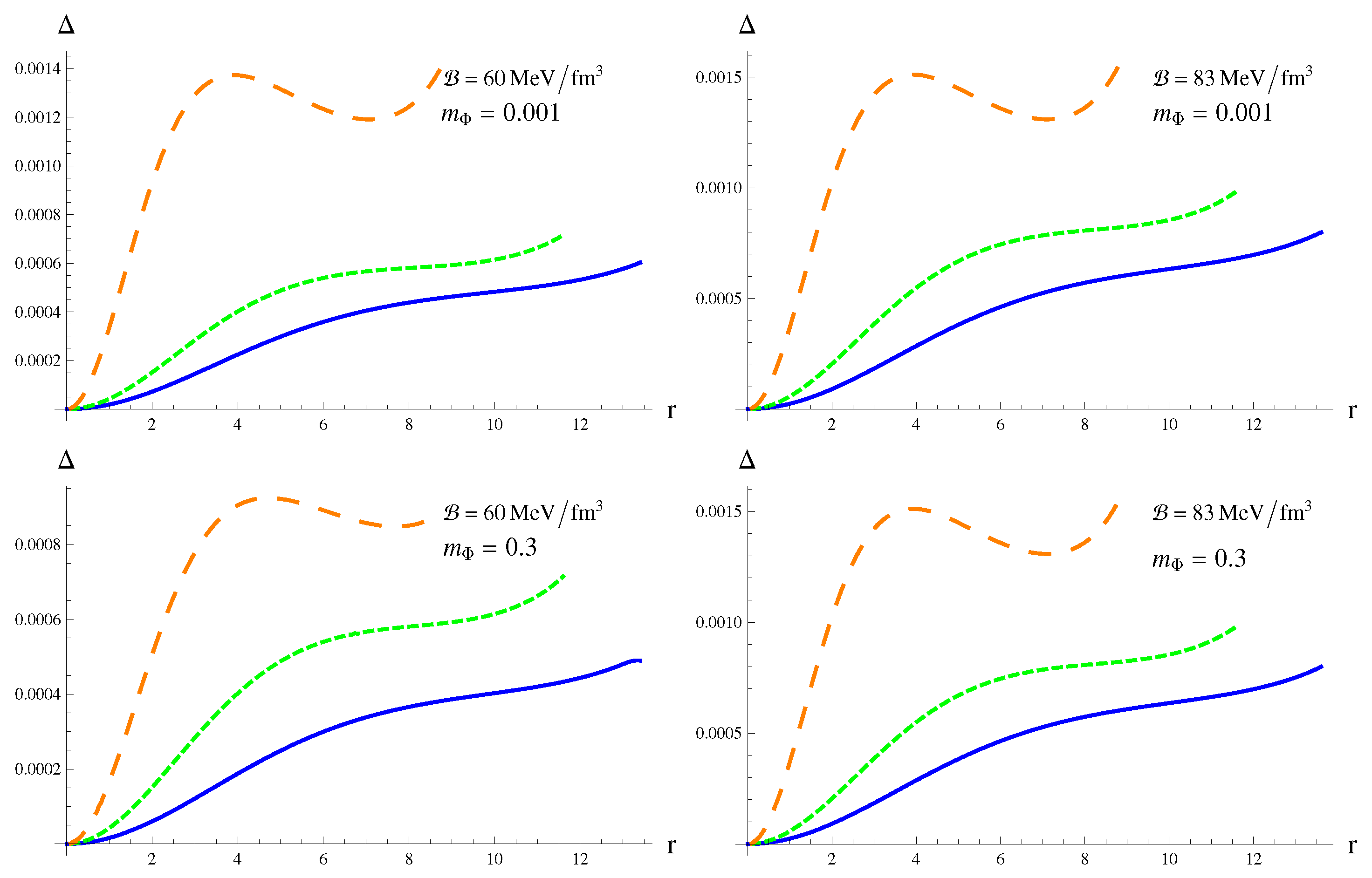
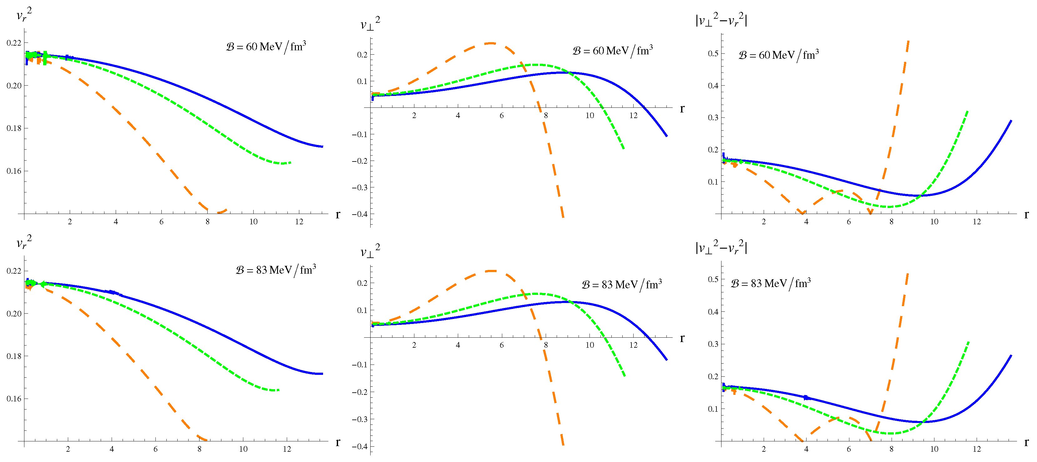
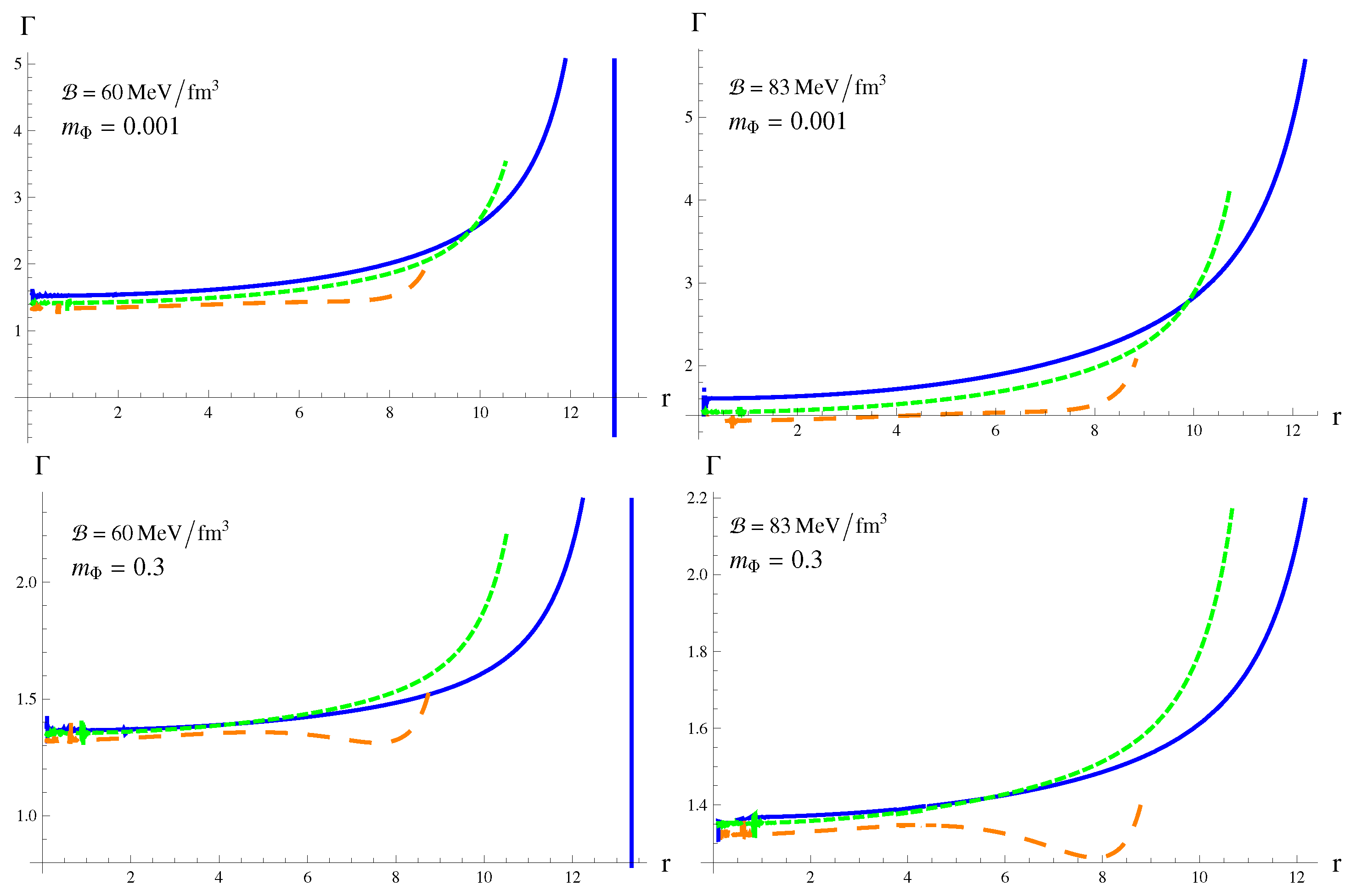
3.3. Stability of Anisotropic Stellar Model

In this section, the anisotropic model is checked for stability via three approaches: causality condition [65], Herrera’s cracking approach [66] and adiabatic index. Causality condition enforces the relation between cause and effect within the stellar region. The condition holds when sound waves travel at a speed less than that of light, i.e., 0 < v r 2 < 1 and 0 < v 2 < 1 , where v r 2 = d p r d ρ and v 2 = d p d ρ are the radial and tangential components of sound speed, respectively. On the other hand, the cracking approach provides a criterion for potentially stable systems. The phenomenon of internal perturbations changing the sign of the radial forces is known as cracking. According to this approach, the condition for a region free from cracking is 0 < | v 2 v r 2 | < 1 . Figure 7 indicates that the system corresponding to m Ψ = 0.001 is unstable as tangential velocity becomes negative near the stellar surface. However, the system is compatible with Herrera’s cracking approach for higher vales of the coupling parameter. The plots in Figure 8 adhere to the criteria of causality and cracking approaches. Thus, a stable structure is obtained for m Ψ = 0.3 .
If an increase in density results in an effective increase in pressure, the system obeys a stiff EoS. A structure associated with a stiff EoS is harder to compress and more stable as compared to a setup with a soft EoS. The stiffness of EoS is measured through adiabatic index given as
Γ = p r + ρ p r d p r d ρ = p r + ρ p r v r 2 .
The lower limit of adiabatic index for a stable anisotropic distribution is 4 3 [67]. The adiabatic index for different values of m Ψ , ω B D and B is displayed in Figure 9. The anisotropic configuration is stable according to this criterion when
  • m Ψ = 0.001 , ω B D = 5 , 8 , B = 60 MeV/fm 3 .
  • m Ψ = 0.001 , ω B D = 8 , 10 , B = 83 MeV/fm 3 .
  • m Ψ = 0.3 , ω B D = 8 , B = 60 MeV/fm 3 .
  • m Ψ = 0.3 , ω B D = 8 , 10 , B = 83 MeV/fm 3 .

4. Concluding Remarks

Astrophysicists have studied the dynamics of stellar structures and their remnants to gain insight into the mechanism of the universe. One of the hypothesized remnants are the quark stars that emerge from the collapse of neutron stars. The interaction among constituent quarks (up, down and strange) of these dense celestial structures is represented by the MIT bag model. In this paper, we have investigated the existence and stability of quark stars in the framework of MBD gravity. For this purpose, we have constructed field equations using well-behaved TK metric potentials and MIT bag model. The unknown constants appearing in the anisotropic model have been specified by matching the interior TK spacetime to exterior Schwarzschild spacetime. The solution has been determined by choosing the potential function as V ( Ψ ) = 1 2 m Ψ 2 Ψ 2 . Moreover, the wave equation has been solved numerically for m Ψ = 0.001 , 0.3 , ω B D = 5 , 8 , 10 and B = 60 MeV/fm 3 , 83 MeV/fm 3 . Finally, we have explored the behavior of matter variables as well as viability and stability of the resulting model in the presence of a massive scalar field.
The observed mass of the strange star candidate PSR J1614-2230 has been used to maximize the anisotropy at r = R and predict the radius of the stellar structure. The predicted radius presented in Table 1 and Table 2 increases with an increase in the values of the bag constant and coupling parameter. The behavior of matter variables shows that the cosmic object becomes denser as the value of the bag constant increases. Moreover, these variables attain a maximum value at the center and decrease towards the surface. The anisotropy increases with an increase in the values of the bag constant. However, an increase in m Ψ or ω B D reduces the anisotropic pressure within the star. Three energy conditions (NEC, WEC, SEC) are readily satisfied for all values of the involved parameters. The model violates the DEC near the boundary for m Ψ = 0.001 . On the other hand, the anisotropic structure becomes viable for m Ψ = 0.3 except for ω B D = 5 .
We have also analyzed the effective mass, compactness and redshift parameter of the constructed model. An increase in the mass of scalar field and value of the bag constant leads to massive and more compact structures with higher redshift parameter (refer to Table 4). It is worth mentioning here that compactness and redshift parameters obey their respective upper bounds [63,64]. The stability of the stellar model has been investigated through three criteria. The tangential velocity becomes negative at the surface of the star when m Ψ = 0.001 for the chosen values of the bag constant and coupling parameter. However, the model is stable according to causality and cracking criteria for m Ψ = 0.3 . Finally, the plots in Figure 9 indicate that the adiabatic index is less than 4 3 for some values of the parameters. It is concluded that viable and stable solutions have been obtained in MBD theory for m Ψ = 0.3 when
  • ω B D = 8 and B = 60 MeV/fm 3 .
  • ω B D = 8 , 10 and B = 83 MeV/fm 3 .
It is worthwhile to mention here that all our results reduce to GR for ω B D .

Author Contributions

Conceptualization, M.S.; Investigation, A.M.; Supervision, M.S.; Writing—original draft, A.M.; Writing—review & editing, M.S. All authors have read and agreed to the published version of the manuscript.

Funding

This research received no external funding.

Conflicts of Interest

The authors declare no conflict of interest.

References

  1. Baade, W.; Zwicky, F. Remarks on super-novae and cosmic rays. Phys. Rev. 1934, 46, 76–77. [Google Scholar] [CrossRef]
  2. Hewish, A.; Bell, S.J.; Pilkington, J.D.H.; Scott, P.F.; Collins, R.A. Observation of a rapidly pulsating radio source. Nature 1968, 217, 709–713. [Google Scholar] [CrossRef]
  3. Witten, E. Cosmic separation of phases. Phys. Rev. D 1984, 30, 272–285. [Google Scholar] [CrossRef]
  4. Ofek, E.O.; Cameron, P.B.; Kasliwal, M.M.; Gal-Yam, A.; Rau, A.; Kulkarni, S.R.; Fraol, D.A.; Chandra, P.; Cenko, S.B.; Soderberg, A.M.; et al. SN2006gy: An extremely luminoue supernova in the galaxy NGC 1260. Astrophys. J. 2007, 659, L13. [Google Scholar] [CrossRef]
  5. Ouyed, R.; Leahy, D.; Jaikumar, P. Predictions for signatures of the quark-nova in superluminous supernovae. arXiv 2009, arXiv:0911.5424. [Google Scholar]
  6. Ruderman, A. Pulsars: Structures and dynamics. Annu. Rev. Astron. Astrophys. 1972, 10, 427–476. [Google Scholar] [CrossRef]
  7. Bowers, R.L.; Liang, E.P.T. Anisotropic spheres in general relativity. Astrophys. J. 1974, 188, 657–665. [Google Scholar] [CrossRef]
  8. Sokolov, A.I. Phase transitions in a superfluid neutron liquid. Sov. Phys. JETP. 1980, 79, 1137–1140. [Google Scholar]
  9. Kippenhahn, R.; Weigert, A. Stellar Structure and Evolution, 2nd ed.; Springer: New York, NY, USA, 1990. [Google Scholar]
  10. Weber, F. Pulsars as Astrophysical Observatories for Nuclear and Particle Physics, 1st ed.; CRC Press: New York, NY, USA, 1999. [Google Scholar]
  11. Herrera, L.; Santos, N.O. Local anisotropy in self-gravitating systems. Phys. Rep. 1997, 286, 53–130. [Google Scholar] [CrossRef]
  12. Harko, T.; Mak, M.K. Anisotropic relativistic stellar models. Ann. Phys. 2002, 11, 3–13. [Google Scholar] [CrossRef]
  13. Hossein, S.M.; Rahaman, F.; Naskar, J.; Kalam, M.; Ray, S. Anisotropic compact stars with variable cosmological constant. Int. J. Mod. Phys. D 2012, 21, 1250088. [Google Scholar] [CrossRef] [Green Version]
  14. Paul, B.C.; Deb, R. Relativistic solutions of anisotropic compact objects. Astrophys. Space Sci. 2014, 354, 421–430. [Google Scholar] [CrossRef]
  15. Maurya, S.K.; Banarjee, A.; Jasim, M.K.; Kumar, J.; Prasad, A.K.; Pradhan, A. Anisotropic compact stars in the Buchdahl model: A comprehensive study. Phys. Rev. D 2019, 99, 044029. [Google Scholar] [CrossRef] [Green Version]
  16. Alcock, C.; Olinto, A.V. Exotic phases of hardonic matter and their astrophysical application. Annu. Rev. Nucl. Part. Sci. 1988, 38, 161–184. [Google Scholar] [CrossRef]
  17. Madsen, J. Physics and astrophysics of strange quark matter. Lect. Notes Phys. 1999, 516, 162–203. [Google Scholar]
  18. Bordbar, G.H.; Peivand, A.R. Computation of the structure of a magnetized strange quark star. Res. Astron. Astrophys. 2011, 11, 851–862. [Google Scholar] [CrossRef]
  19. Abbott, B.P.; Abbott, R.; Abbott, T.D.; Acernese, F.; Ackley, K.; Adams, C.; Adams, T.; Addesso, P.; Adhikari, R.X.; Adya, V.B.; et al. GW170817: Observation of gravitational waves from a binary neutron star inspiral. Phys. Rev. Lett. 2017, 119, 161101. [Google Scholar] [CrossRef] [PubMed] [Green Version]
  20. Abbott, B.P.; Abbott, R.; Abbott, T.D.; Abraham, S.; Acernese, F.; Ackley, K.; Adams, C.; Adhikari, R.X.; Adya, V.B.; Affeldt, C.; et al. GW190425: Observation of a compact binary coalescence with total mass ∼3.4M. Astrophys. J. Lett. 2020, 892, L3. [Google Scholar] [CrossRef]
  21. Farhi, E.; Jaffe, R.L. Strange matter. Phys. Rev. D 1984, 30, 2379. [Google Scholar] [CrossRef]
  22. Stergioulas, N. Rotating stars in relativity. Living Rev. Relativ. 2003, 6, 3. [Google Scholar] [CrossRef] [Green Version]
  23. Xu, R.X. What can the redshift observed in exo 0748-676 tell us? Chin. J. Astron. Astrophys. 2003, 3, 33–37. [Google Scholar] [CrossRef] [Green Version]
  24. Rahaman, F.; Sharma, R.; Ray, S.; Maulick, R.; Karar, I. Strange stars in Krori-Barua spacetime. Eur. Phys. J. C 2012, 72, 2071. [Google Scholar] [CrossRef]
  25. Kalam, M.; Usmani, A.A.; Rahaman, F.; Hossein, S.M.; Karar, I.; Sharma, R. A relativistic model for strange quark star. Int. J. Theor. Phys. 2013, 52, 3319. [Google Scholar] [CrossRef]
  26. Haensel, P.; Zdunik, J.L.; Schaffer, R. Strange quark stars. Astron. Astrophys. 1986, 160, 121–128. [Google Scholar]
  27. Cheng, K.S.; Dai, Z.G.; Lu, T. Strange stars and related astrophysical phenomena. Int. J. Mod. Phys. D 1998, 7, 139–176. [Google Scholar] [CrossRef]
  28. Harko, T.; Mak, M.K. An exact anisotropic quark star model. Chin. J. Astron. Astrophys. 2002, 2, 248–259. [Google Scholar]
  29. Rahaman, F.; Chakraborty, K.; Kuhfittig, P.K.F.; Shit, G.C.; Rahman, M. A new deterministic model of strange stars. Eur. Phys. J. C 2014, 74, 3126. [Google Scholar] [CrossRef] [Green Version]
  30. Bhar, P. A new hybrid star model in Krori-Barua spacetime. Astrophys. Space Sci. 2015, 357, 46. [Google Scholar] [CrossRef]
  31. Maurya, S.K.; Gupta, Y.K.; Ray, S.; Chowdhury, S.R. Spherically symmetric charged compact stars. Eur. Phys. J. C 2015, 75, 389. [Google Scholar] [CrossRef] [Green Version]
  32. Maurya, S.K.; Jasim, M.K.; Gupta, Y.K.; Smitha, T.T. A new model for charged anisotropic compact star. Astrophys. Space Sci. 2016, 361, 163. [Google Scholar] [CrossRef] [Green Version]
  33. Murad, M.H. Some analytical models of anisotropic strange stars. Astrophys. Space Sci. 2016, 361, 20. [Google Scholar] [CrossRef]
  34. Deb, D.; Chowdhury, S.R.; Ray, S.; Rahaman, F.; Guha, B.K. Relativistic model for anisotropic strange stars. Ann. Phys. 2017, 387, 239–252. [Google Scholar] [CrossRef] [Green Version]
  35. Bhar, P. Anisotropic compact star model: A brief study via embedding. Eur. Phys. J. C 2019, 79, 138. [Google Scholar] [CrossRef] [Green Version]
  36. Dirac, P.A.M. The cosmological constants. Nature 1937, 139, 323. [Google Scholar] [CrossRef]
  37. Dirac, P.A.M. A new basis for cosmology. Proc. R. Soc. Lond. A 1938, 165, 199–208. [Google Scholar] [CrossRef] [Green Version]
  38. Brans, C.; Dicke, R.H. Mach’s principle and a relativistic theory of gravitation. Phys. Rev. 1961, 124, 925–935. [Google Scholar] [CrossRef]
  39. Will, C.M. Theory and experiment in gravitational physics. Living Rev. Rel. 2001, 4, 4. [Google Scholar] [CrossRef] [Green Version]
  40. Weinberg, E.J. Some problems with extended inflation. Phys. Rev. D 1989, 40, 3950. [Google Scholar] [CrossRef]
  41. Perivolaropoulos, L. PPN parameter γ and solar system constraints of massive Brans–Dicke theories. Phys. Rev. D 2010, 81, 047501. [Google Scholar] [CrossRef] [Green Version]
  42. Sotani, H. Slowly rotating relativistic stars in scalar-tensor gravity. Phys. Rev. D 2012, 86, 124036. [Google Scholar] [CrossRef] [Green Version]
  43. Silva, H.O.; Macedo, C.F.B.; Beri, E.; Crispino, L.C.B. Slowly rotating anisotropic neutron stars in general relativity and scalar-tensor theory. Class. Quantum Grav. 2015, 32, 145008. [Google Scholar] [CrossRef]
  44. Doneva, D.D.; Yazadjiev, S.S. Rapidly rotating neutron stars with a massive scalar field-striucture and universal relations. J. Cosmol. Astropart. Phys. 2016, 11, 019. [Google Scholar] [CrossRef]
  45. Staykov, K.V.; Popchev, D.; Doneva, D.D.; Yazadjiev, S.S. Static and slowly rotating neutron stars in scalar-tensor theory with a massive scalar field. Eur. Phys. J. C 2018, 78, 586. [Google Scholar] [CrossRef] [Green Version]
  46. Astashenok, A.V. Neutron and quark stars in f( R ) gravity. Int. J. Mod. Phys. Conf. Ser. 2016, 41, 1660130. [Google Scholar] [CrossRef] [Green Version]
  47. Sharif, M.; Waseem, A. Anisotopic quark stars in f( R ,T) gravity. Eur. Phys. J. C 2018, 78, 868. [Google Scholar] [CrossRef]
  48. Deb, D.; Ketov, S.V.; Khlopov, M.; Ray, S. Study on charged stars in f( R ,T) gravity. J. Cosmol. Astropart. Phys. 2019, 10, 70. [Google Scholar] [CrossRef] [Green Version]
  49. Maurya, S.K.; Errehymy, A.; Deb, D.; Tello-Ortiz, F.; Daoud, M. Study of anisotropic stange stars in f( R ,T) gravity: An embedding approach under the simplest linear functinal of the matter-geometry coupling. Phys. Rev. D 2019, 100, 044014. [Google Scholar] [CrossRef] [Green Version]
  50. Sharif, M.; Majid, A. Anisotropic strange stars through embedding technique in massive Brans–Dicke gravity. Eur. Phys. J. Plus 2020, 135, 558. [Google Scholar] [CrossRef]
  51. Tolman, R.C. Static solutions of Einstein’s field equations for spheres of fluids. Phys. Rev. 1939, 55, 364–373. [Google Scholar] [CrossRef] [Green Version]
  52. Kuchowicz, B. General relativistic fluid spheres. I. New solutions for sphericlly symmetric matter distributions. Acta. Phys. Pol. 1968, 33, 541–563. [Google Scholar]
  53. Jasim, M.K.; Deb, D.; Ray, S.; Gupta, Y.K.; Chowdhury, S.R. Anisotropic strange stars in Tolman–Kuchowicz spacetime. Eur. Phys. J. C 2018, 78, 603. [Google Scholar] [CrossRef] [Green Version]
  54. Biswas, S.; Shee, D.; Ray, S.; Rahaman, F.; Guha, B.K. Relativistic strange stars in Tolman–Kuchowicz spacetime. Ann. Phys. 2019, 409, 167905. [Google Scholar] [CrossRef] [Green Version]
  55. Shamir, M.F.; Naz, T. Study of charged stellar models in f( G ) gravity with Tolman–Kuchowicz spacetime. Int. J. Mod. Phys. A 2020, 35, 2050040. [Google Scholar]
  56. Yazadjiev, S.S.; Doneva, D.D.; Popchev, D. Slowly rotating neutron stars in scalar-tensor theories with a massive scalar field. Phys. Rev. D 2016, 93, 084038. [Google Scholar] [CrossRef] [Green Version]
  57. Bruckman, W.F.; Kazes, E. Properties of the solutions of cold ultradense configurations in the Brans–Dicke theory. Phys. Rev. D 1977, 16, 2. [Google Scholar] [CrossRef]
  58. O’Brien, S.; Synge, J.L. Jump Conditions at Discontinuities in General Relativity; Dublin Institute for Advanced Studies: Dublin, Ireland, 1952. [Google Scholar]
  59. Demorest, P.B.; Pennucci, T.; Ransom, S.M.; Roberts, M.S.E.; Hessels, J.W.T. A two-solar-mass neutron star measured using Shapiro delay. Nature 2010, 467, 1081–1083. [Google Scholar] [CrossRef]
  60. Kalam, M.; Rahaman, F.; Ray, S.; Hossein, S.M.; Karar, I.; Naskar, J. Anisotropic strange star with de sitter spacetime. Eur. Phys. J. C 2012, 72, 2248. [Google Scholar] [CrossRef]
  61. Lake, K. All static spherically symmetric perfect-fluid solutions of Einstein’s equations. Phys. Rev. D 2003, 67, 104015. [Google Scholar] [CrossRef] [Green Version]
  62. Fujii, Y.; Maeda, K. The Scalar-Tensor Theory of Gravitation; Landshoff, P.V., Nelson, D.R., WeinBerg, S., Eds.; Cambridge University Press: Cambridge, UK, 2003. [Google Scholar]
  63. Buchdahl, H.A. General relativistic fluid spheres. Phys. Rev. 1959, 116, 1027–1034. [Google Scholar] [CrossRef]
  64. Ivanov, B.V. Maximum bounds on the surface redshift of anisotropic stars. Phys. Rev. D 2002, 65, 104011. [Google Scholar] [CrossRef] [Green Version]
  65. Abreu, H.; Hernandez, H.; Nunez, L.A. Sound speeds, cracking and stability of self-gravitating anisotropic compact objects. Class. Quantum Gravit. 2007, 24, 4631–4645. [Google Scholar] [CrossRef]
  66. Herrera, L. Cracking of self-gravitating compact objects. Phys. Lett. A 1992, 165, 206–210. [Google Scholar] [CrossRef]
  67. Heintzmann, H.; Hillebrandt, W. Neutron stars with an anisotropic equation of state: Mass, redshift and stability. Astron. Astrophys. 1975, 24, 51–55. [Google Scholar]
Figure 1. Metric potentials for massive scalar field versus radial (in km).
Universe 06 00124 g001
Figure 2. Matter variables (in km 2 ) as functions of r (in km) with m Ψ = 0.001 .
Universe 06 00124 g002
Figure 3. Matter variables (in km 2 ) as functions of r (in km) with m Ψ = 0.3 .
Universe 06 00124 g003
Figure 4. Effective anisotropy (in km 2 ) as a function of r (in km).
Universe 06 00124 g004
Figure 5. DEC (with ρ , p r , p in k m 2 ) against the radial coordinate (in km) for m Ψ = 0.001 .
Universe 06 00124 g005
Figure 6. DEC (with ρ , p r , p in km 2 ) against the radial coordinate m Ψ = 0.3 .
Universe 06 00124 g006
Figure 7. Radial/tangential velocities and | v 2 v r 2 | with m Ψ = 0.001 .
Universe 06 00124 g007
Figure 8. Radial /tangential velocities and | v 2 v r 2 | with m Ψ = 0.3 .
Universe 06 00124 g008
Figure 9. Plots of adiabatic index versus r.
Universe 06 00124 g009
Table 1. Physical properties of PSR J1614-2230 ( M = 1.97 ± 0.04 M ) with m Ψ = 0.001 .
B = 60 MeV/fm 3
ω B D Ψ c Predicted ρ c (gm/cm 3 ) ρ s (gm/cm 3 ) p c (dyne/cm 2 )
Radius (km)
50.1 8.8024 0.1813 + 0.1815 2.3051 × 10 16 7.2604 × 10 14 3.9692 × 10 36
80.125 11.5653 0.2426 + 0.243 9.0518 × 10 15 4.0282 × 10 14 1.4958 × 10 36
100.15 13.4483 0.2869 + 0.2878 6.8805 × 10 15 3.6403 × 10 14 1.1523 × 10 36
B = 83 MeV/fm 3
ω B D Ψ c Predicted ρ c (gm/cm 3 ) ρ s (gm/cm 3 ) p c (dyne/cm 2 )
Radius (km)
50.1 8.828 0.1829 + 0.1832 2.5432 × 10 16 6.0511 × 10 14 4.3768 × 10 36
80.18 11.6418 0.2478 + 0.2482 1.2336 × 10 16 5.2002 × 10 14 2.1006 × 10 36
100.25 13.5868 0.296 + 0.2975 9.0211 × 10 15 4.3507 × 10 14 1.5319 × 10 36
Table 2. Physical properties of PSR J1614-2230 ( M = 1.97 ± 0.04 M ) with m Ψ = 0.3 .
B = 60 MeV/fm 3
ω B D Ψ c Predicted ρ c (gm/cm 3 ) ρ s (gm/cm 3 ) p c (dyne/cm 2 )
Radius (km)
50.1 8.8024 0.1813 + 0.1815 1.5412 × 10 16 1.2272 × 10 15 2.4962 × 10 36
80.125 11.5653 0.2426 + 0.243 9.3622 × 10 15 8.3976 × 10 14 1.509 × 10 36
100.15 13.4483 0.2869 + 0.2878 6.4885 × 10 15 9.9402 × 10 14 9.4198 × 10 35
B = 83 MeV/fm 3
ω B D Ψ c Predicted ρ c (gm/cm 3 ) ρ s (gm/cm 3 ) p c (dyne/cm 2 )
Radius (km)
50.1 8.828 0.1829 + 0.1832 2.5687 × 10 16 9.3087 × 10 14 4.4261 × 10 36
80.18 11.6418 0.2478 + 0.2482 1.3305 × 10 16 1.3258 × 10 15 2.1018 × 10 36
100.25 13.5868 0.296 + 0.2975 9.7515 × 10 15 1.0625 × 10 15 1.5094 × 10 36
Table 3. Critical values of m Ψ for different values of B and ω B D corresponding to PSR J1614-2230 ( M = 1.97 ± 0.04 M ).
B = 60 MeV/fm 3 B = 83 MeV/fm 3
ω B D m Ψ ω B D m Ψ
50.750.65
80.380.25
100.2100.15
Table 4. Values of μ s and Z s for different values of m Ψ , B and ω B D corresponding to PSR J1614-2230 ( M = 1.97 ± 0.04 M ).
m Ψ = 0.001
B = 60 MeV/fm 3 B = 83 MeV/fm 3
ω B D μ s Z s μ s Z s
50.02910.03030.03260.0338
80.03110.03260.04410.0468
100.03860.04060.05220.0571
m Ψ = 0 . 3
B = 60 MeV/fm 3 B = 83 MeV/fm 3
ω B D μ s Z s μ s Z s
50.03540.03700.03600.0381
80.03870.04120.06130.0667
100.04740.05140.09760.1146

