Article

Evidence of Time Evolution in Quantum Gravity

by
Sergey Cherkas
1,† and
Vladimir Kalashnikov
2,*,†
1
Institute for Nuclear Problems, Bobruiskaya 11, 220030 Minsk, Belarus
2
Dipartimento di Ingegneria dell’Informazione, Elettronica e Telecomunicazioni, Sapienza Universitá di Roma, Via Eudossiana 18, 00189 Roma, Italy
*
Author to whom correspondence should be addressed.
These authors contributed equally to this work.
Universe 2020, 6(5), 67; https://doi.org/10.3390/universe6050067
Submission received: 1 April 2020 / Revised: 25 April 2020 / Accepted: 4 May 2020 / Published: 8 May 2020
(This article belongs to the Section Gravitation)

Abstract

:
In this paper, we argue that the problem of time is not a crucial issue inherent in the quantum picture of the universe evolution. On the minisuperspace model example with the massless scalar field, we demonstrate four approaches to the description of quantum evolution, which give similar results explicitly. The relevance of these approaches to building a quantum theory of gravity is discussed.

Graphical Abstract

1. Introduction

Usually, some crucial theoretical problems were self-created in some sense, and then these issues were solved successfully during some period. An example could be the spin crisis problem, which had been stating about 30 years ago [1]. The problem of time [2,3,4,5,6] held for a relatively long time from [7] and was related closely with the variety of the points of view in a gravity quantization [8]. The root of this issue is the gauge invariance of the general relativity [9].1 Such invariance allows for choosing the equivalent time parameterizations, and one may suspect that the time is an “illusion” [10].
On the other hand, astrophysical data demonstrate the time evolution of the universe. The modern trends in the interpretation of quantum mechanics (e.g., see [11]) suggest that all the phenomena, including the universe itself, are generally quantum. Thus, the time evolution in the frameworks of quantum cosmology has to be explained.
Although “eternity” and “time” are two sides of one coin [12], all observations are performed in time. Thus, time should put into a theory, in any case, to confront the theory with observations. However, sometimes, it could be useful to think in terms of eternity for the development of theoretical concepts, such as sub specie aeternitatis.
The complexity of the full system of the equations of gravity does not prevent considering this problem as an example of the so-called minisuperspace models [13], which are extremely simple but have the Hamiltonian constraint like that in the general case.
Here we show that the problem of time does not prevent calculating the time-dependent mean values, which could be, in the principle, compared with the observations. In the quantization methods considered, the time reparameterization invariance [14] is violated by imposing the gauge condition. As a result, the Schrödinger equation arises in the methods of A, E. If the quantization procedure is realized before imposing the gauge condition (the methods B, C, D), the WDW equation arises. After that, the gauge condition is set in the scalar product (the methods B, C), or at a level of the operator equations of motion (the method D).

2. Classical Picture

As is well-known, there is no problem with defining time in the classical theory because it implies that if an observer has some particular clock, she can choose a gauge corresponding to this clock.
Let us consider an action for gravity and a real massless scalar field ϕ :
S = 1 16 π G R g d 4 x + 1 2 μ ϕ g μ ν ν ϕ g d 4 x ,
where R is a scalar curvature.
We restrict the consideration by the uniform, isotropic and flat universe
d s 2 = g μ ν d x μ d x ν = a 2 ( N 2 d η 2 d 2 r ) ,
where a scale factor a and a lapse function N depend on a conformal time η only. Under these conditions, the action of Equation (1) becomes
S = 1 2 1 N M p 2 a 2 + a 2 ϕ 2 d η ,
where the reduced Planck mass M p = 3 4 π G is used2, which is set to unity for simplicity.
The action (Equation (3)) in the generalized form [15,16,17,18,19] looks as
S = p a a + π ϕ ϕ N 1 2 p a 2 + π ϕ 2 2 a 2 d η .
The variation of Equation (4) with respect to π ϕ and p a gives π ϕ = ϕ a 2 / N and p a = a / N , respectively. After substituting these values into Equation (4), Equation (3) is recovered. The explicit expression for the Hamiltonian follows from Equation (4):
H = N 1 2 p a 2 + π ϕ 2 2 a 2 ,
which is also the Hamiltonian constraint
Φ 1 = 1 2 p a 2 + π ϕ 2 2 a 2 = 0 ,
due to δ S δ N = 0 .
Time evolution of an arbitrary quantity is expressed through the Poisson brackets
d A d η = A η + { H , A } ,
which reads as
{ A , B } = A π ϕ B ϕ A ϕ B π ϕ A p a B a + A a A p a .
The full system of the equations of motion has the form:
π ϕ = H ϕ = 0 , π ϕ = c o n s t k , ϕ = H π ϕ = k a 2 , a = H p a = p a , p a = H a = k 2 a 3 .
The solution of the equations of motion is
a = 2 | π ϕ | η , ϕ = π ϕ 2 | π ϕ | ln η + c o n s t .
According to Equation (10), a gauge fixing condition
Φ 2 = a 2 | π ϕ | η = 0 ,
which conserves in time, can be introduced in addition to the constraint Φ 1 .
One can see that there is an explicit time evolution under some particular gauge fixing. Moreover, for this simple example, the system could be reduced to a single degree of freedom [20,21].
Let us take π ϕ and ϕ as the physical variables, then a and p a have to be excluded by the constraints in Equations (6) and (11). Substituting p a , a and a into Equation (3) results in
S = π ϕ ϕ H p h y s ( ϕ , π ϕ , η ) d η ,
where
H p h y s ( ϕ , π ϕ , η ) = p a a = | π ϕ | 2 η .

3. Quantum Pictures with Time

3.1. The Schrödinger Equation with a Physical Hamiltonian (Method A)

The most simple and straightforward way to the description of the quantum evolution is based on the Schröodinger equation [20,21]
i η Ψ = H ^ p h y s Ψ
with a physical Hamiltonian Equation (13). In the momentum representation, the operators become
π ^ ϕ = k , ϕ ^ = i k .
The solution of Equation (14) is
Ψ ( k , η ) = C ( k ) | 2 k η | i | k | / 2 e i | k | / 2 ,
where C ( k ) is a momentum wave packet. An arbitrary operator A ^ build from ϕ ^ = i k and a = 2 | k | η is, in fact, the function of η , k, and i k . Using the wave function Equation (16) allows us to calculate the mean value
< C | A ^ | C > = Ψ * ( k , η ) A ^ Ψ ( k , η ) d k .
Since the base wave functions ψ k = | 2 k η | i | k | / 2 e i | k | / 2 contain the module of k, a singularity may arise at k = 0 if A ^ contains the degrees of the differential operator k . That could violate hermicity. To avoid this, the wave packet C ( k ) should turn to zero at k = 0 . For instance, it could be taken in the form of the Gaussian function multiplied by k 2
C ( k ) = 4 σ 5 3 π k 2 exp k 2 2 σ 2 .
Let us come to the calculation of the concrete mean values taking σ = 1 for simplicity. Mean values of the operators ϕ ^ 2 and a are
< C | a | C > = 4 3 2 π η e k 2 k 9 / 2 d k = 4 3 2 π Γ ( 11 / 4 ) η , < C | ϕ ^ 2 | C > = 1 3 π e k 2 ( 4 k 6 + k 4 20 + ln 2 2 + ln ( η k ) ln ( 4 η k ) 8 k 2 + 2 i k 3 2 k 2 ln ( 2 η k ) + 4 ln ( η k ) + 4 ln 2 + 1 ) d k =
1 12 ln η ( 3 ln η 3 γ + 8 ) + π 2 32 + γ 2 16 γ 3 + 4 3 ,
where Γ is the Gamma function, and γ is the Euler constant. Let us note that the imaginary part in Equation (20) disappears after integration on k due to hermicity of ϕ ^ . Figure 1 demonstrates the infiniteness of the mean-square value of ϕ at η = 0 , then it decreases and begins to increase finally. Examples of software calculating mean values are supplemented [22] (see Supplementary).
Another more complicated example is
< C | ϕ ^ 2 a + a ϕ ^ 2 | C > = 1 3072 ( 16 ln η ( ln η ( 4 ln η ( 3 ln η 6 γ + 16 ) + 9 π 2 + 6 γ ( 3 γ 16 ) + 384 ) 9 γ π 2 + 24 π 2 6 γ ( 64 + ( γ 8 ) γ ) + 800 ) + 224 ζ ( 3 ) ( 6 ln η + 3 γ 8 ) + 21 π 4 + 12 γ ( 3 γ 16 ) π 2 + 768 π 2 + 4 γ γ ( 384 + γ ( 3 γ 32 ) ) 1600 + 16640 ) ,
where ζ ( x ) is the Zeta-function. The time dependence in Equation (21) arises from two sources: the time-dependent wave function in Equation (17) and a = 2 | k | η .

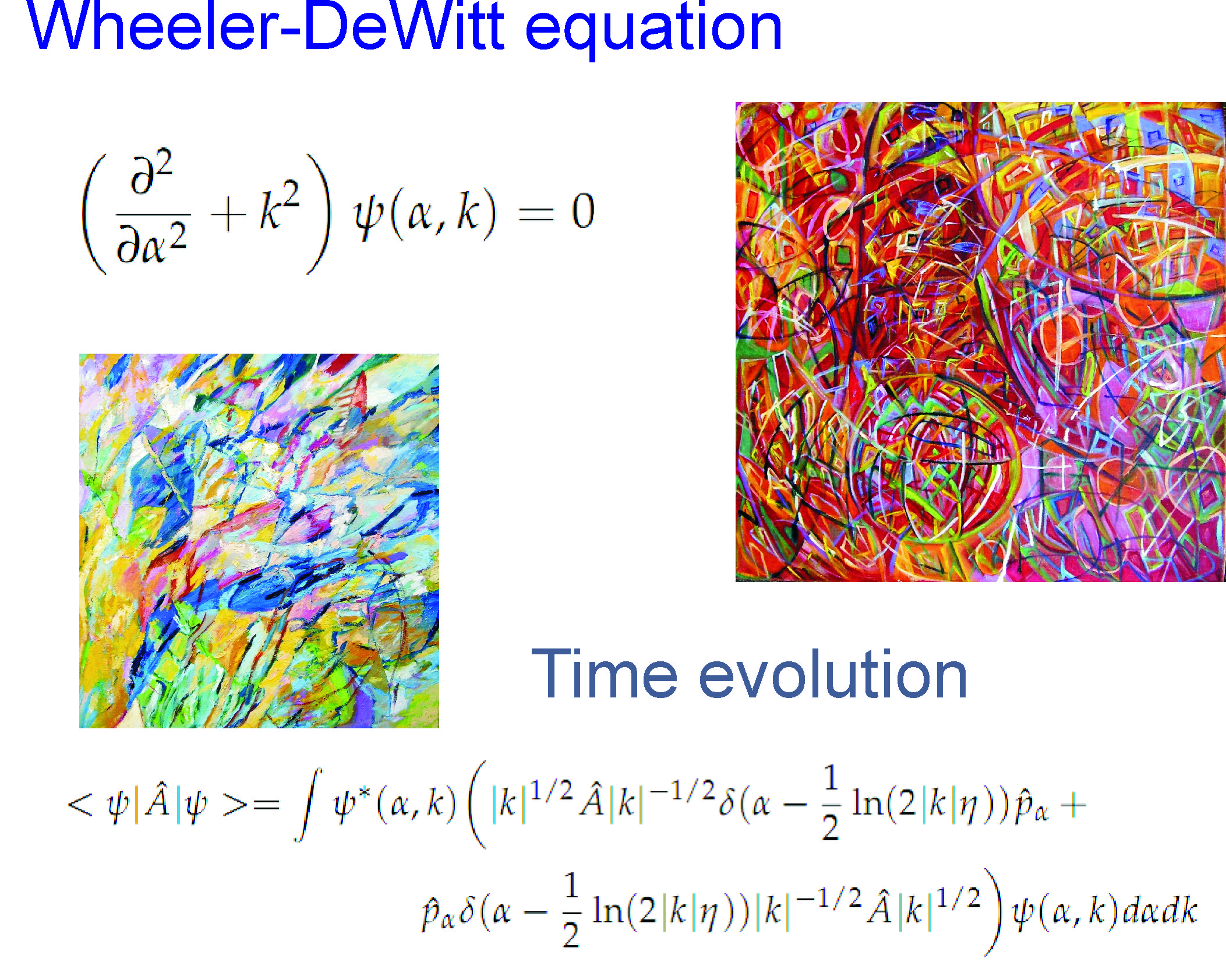
3.2. Time Evolution from the WDW Equation (Method B)

The problem of time began from the discussion of the WDW equation [7,9,20,23,24], which is a workhorse of quantum cosmology and a mathematical implementation of eternity. It is often stated that the WDW equation does not contain time explicitly. Indeed, it is true. Nevertheless, the WDW equation does not forbid a time evolution if one considers a full quantum picture, including gauge fixing and evaluation of the mean values of the operators [25]3. The point is that the WDW equation has to be supplemented by the scalar product.
Let us to introduce the variable α = ln a and perform the canonical quantization
[ p ^ α , α ] = i , [ π ^ ϕ , ϕ ] = i
of the constraint Φ 1 = 0 . That results in the WDW equation
2 α 2 2 ϕ 2 Ψ ( α , ϕ ) = 0
of the Klein–Gordon type.
Scalar products for the Klein–Gordon equation are discussed in [18,26,27,28], where the “current” and “density” [26] products were proposed. Here we use only the scalar product of the “current” type:
< Ψ | Ψ > = i Ψ * ( α , ϕ ) α Ψ ( α , ϕ ) Ψ ( α , ϕ ) α Ψ * ( α , ϕ ) | α = α 0 d ϕ ,
including the hyperplane α = α 0 . For a mean value of some operator, the following expression could be introduced (see the last formula in [26])
< Ψ | A ^ | Ψ > = i Ψ * D ^ 1 / 4 A ^ D ^ 1 / 4 Ψ α Ψ * α D ^ 1 / 4 A ^ D ^ 1 / 4 Ψ | α = α 0 d ϕ ,
where D ^ = 2 ϕ 2 . In the momentum representation π ^ ϕ = k , ϕ ^ = i k , the WDW Equation (23) reads as
2 α 2 + k 2 ψ ( α , k ) = 0 ,
and, as a result of D ^ 1 / 2 = | k | , the scalar product of Equation (25) takes the form:
< Ψ | A ^ | Ψ > = i C * ( k ) e i | k | α A ^ e i | k | α C ( k ) | α = α 0 d k ,
where
Ψ ( α , ϕ ) = e i k ϕ ψ ( α , k ) d k = e i k ϕ i | k | α 2 | k | C ( k ) d k
is taken. To introduce the time evolution into this picture, one has to choose a time-dependent integration plane in Equation (27) instead of α = α 0 by writing α = 1 2 ln 2 | k | η according to Equation (11), i.e., to Φ 2 = 0 .
However, if the operator A ^ ( α , k , i α , i k ) contains differentiation k or α , hermicity could be lost. To prevent this, let us rewrite Equations (25) and (27) in the form of
< ψ | A ^ | ψ > = ψ * ( α , k ) ( | k | 1 / 2 A ^ | k | 1 / 2 δ ( α 1 2 ln ( 2 | k | η ) ) p ^ α + p ^ α δ ( α 1 2 ln ( 2 | k | η ) ) | k | 1 / 2 A ^ | k | 1 / 2 ) ψ ( α , k ) d α d k ,
where p α = i α and hermicity of A ^ relatively α , k variables are implied. In this case, no problem with hermicity arises if one takes the functions ψ ( α , k ) tending to zero at α ± to provide the throwing over the differential operators / α by the integration by parts. The functions ψ ( α , k ) = e i | k | α 2 | k | C ( k ) do not possess such a property. Thus, we shall take the functions
ψ ( α , k ) = e i | k | α α 2 / Δ 2 | k | C ( k )
in the intermediate calculations and, then, after integration over α , tend Δ to infinity. Performing the concrete calculations with the above wave packet Equation (18), we again obtain the same values for Equations (19) and (20). As for the mean value Equation (21) of Section 3.1, we cannot compare it using this picture because the particular operator ordering a ϕ ^ 2 + ϕ ^ 2 a has been used in Equation (21), but here the operators a = exp α and ϕ ^ commute formally implying an existence of some intrinsic automatic ordering.

3.3. An Evolution from the WDW Using the Grassmann Variables (Method C)

Another version with the anticommutative variables could be proposed in the form
< ψ | A | ψ > = ψ * ( α , k ) exp ( i λ α 1 2 ln ( 2 | k | η ) + θ ¯ θ p ^ α + 1 2 χ ¯ χ | k | i / 2 A ^ | k | i / 2 + | k | i / 2 A ^ | k | i / 2 ) ψ ( α , k ) d λ d α d k d θ d θ ¯ d χ d χ ¯ ,
where the anticommutating Grassmann variables θ i = ( θ , χ ) , θ ¯ i = ( θ ¯ , χ ¯ ) have the following properties: θ i θ j + θ j θ i = 0 , d θ i = 0 , θ i d θ i = 1 , ( θ ¯ i ) * = θ i , ( θ ¯ i θ j ) * = θ ¯ j θ i . Again, for reasons of hermicity, we take the functions of Equation (30) and then tend Δ to infinity. For the practical calculations, it is convenient to separate the expression in the exponent of Equation (31) into two parts M = i λ α 1 2 ln 2 | k | η , and R ^ = θ ¯ θ p ^ α + 1 2 χ ¯ χ | k | i / 2 A ^ | k | i / 2 + | k | i / 2 A ^ | k | i / 2 for using the formula [29]
exp M ^ + R ^ = 1 + m = 1 X ^ m m ! exp M ^ ,
where X ^ m is set recursively as X ^ 1 = R and X ^ m = R ^ X ^ m 1 + [ M ^ , X ^ m 1 ] . In fact, it is sufficient to take only finite number of terms in a sum of Equation (32).

3.4. The quasi-Heisenberg Picture (Method D)

Another approach to consider the time evolution is to take classical equations of motion and then quantize them, i.e., write “hat” over every quantity [30,31,32,33]. The operator equations of motion take the form:
ϕ ^ + 2 α ^ ϕ ^ = 0 , α ^ + α ^ 2 + ϕ ^ 2 = 0 .
One needs to find the commutation relations of the operators α ^ ( η ) , ϕ ^ ( η ) . The problem was solved by Dirac, who has introduced the “Dirac brackets” for a system with constraints postulating that commutator relations of the operators have to be analogous to the Dirac brackets. However, it is not always possible to find an operator realization of this commutator relations. The quasi-Heisenberg picture suggests to find an operator realization only at the initial moment and then allow operators to evolve according to the equations of motion. The initial conditions for operators could be taken in the form
α ^ ( 0 ) = α 0 , α ^ ( 0 ) = e 2 α 0 | k | , ϕ ^ ( 0 ) = i k , ϕ ^ ( 0 ) = e 2 α 0 k .
The solution of the operator equations of motion (Equation (33)) with the initial conditions (Equation (34)) is
α ( η ) = α 0 + 1 2 ln 1 + 2 | k | η e 2 α 0 , ϕ ^ ( η ) = i k + k 2 | k | ln 1 + 2 | k | η e 2 α 0 .
To built the Hilbert space, in which these quasi-Heisenberg operators act, one may use the WDW Equation (23) and the scalar product (Equation (27)) but, at the end of mean values evaluating, the value of α 0 should be set to minus infinity, i.e., α 0 , which corresponds to a 0 at η = 0 . Explicit calculation gives the same mean values as Equations (19)–(21).

3.5. An Evolution Using the Unconstraint Schrödinger Equation in the Extended Space (Method E)

It is believed [14,34,35] that the Grassmann variables allow for writing the Lagrangian without constraints at all. Here, one has two possibilities: to set a gauge imposing an additional condition as a function of p a , a, π ϕ , ϕ such as Equation (11) (canonical gauge). Another alternative is to impose this condition as a function of N (non-canonical gauge).

3.5.1. Canonical Gauge

The discussion can be started in terms of continual integral which gives a transition amplitude from i n to o u t states [14,36,37]:
< o u t | i n > = Z = e i π ϕ ϕ H p h y s ( ϕ , π ϕ ) d η D π ϕ D ϕ ,
where H p h y s is given by Equation (13). This functional can be rewritten in the form
Z = e i π ϕ ϕ p a a N 1 2 p a 2 + π ϕ 2 2 a 2 d η Π η p a Π η δ a 2 η | π ϕ | D p a D a D π ϕ D ϕ D N ,
where [37] p a = { Φ 1 , Φ 2 } is the Faddeev–Popov determinant. Equivalence of Equations (36) and (37) can be checked by transition to a new integration variable a ˜ = a 2 η | π ϕ | , and integrating on a ˜ , N, p a in Equation (37) gradually.
Using the Grassmann anticommutative variables in Equation (37) leads to the form containing the unconstraint Lagrangian in the exponent
Z = e i π ϕ ϕ p a a N 1 2 p a 2 + π ϕ 2 2 a 2 λ a 2 η | π ϕ | θ ¯ θ p a d η D p a D a D π ϕ D ϕ D N D λ D θ D θ ¯ .
Equation (38) allows for writing the Hamiltonian
H = N 1 2 p a 2 + π ϕ 2 2 a 2 + λ a 2 η | π ϕ | + θ ¯ θ p a ,
which, after canonical quantization, could be used to describe evolution as in both Schrödinger and Heisenberg pictures.

3.5.2. Non-Canonical Gauge

Let us remind, how the Faddeev–Popov determinant appears in non-canonical gauge. The action Equation (3) is an invariant relatively the infinitesimal gauge transformations:
a ˜ = a + δ a = a + ε a ,
ϕ ˜ = ϕ + δ ϕ = ϕ + ε ϕ ,
N ˜ = N + δ N = N + ( N ε ) ,
where ε is an infinitesimal function of time. When one sets a non-canonical gauge condition in the form F ( N ) = 0 , the functional integral, including a gauge fixing multiplier with the Dirac δ -function, becomes [14]
Z = e i π ϕ ϕ p a a N 1 2 p a 2 + π ϕ 2 2 a 2 d η Π η δ F δ ε Π η δ ( F ) D p a D a D π ϕ D ϕ D N ,
where again the Faddev–Popov determinant Δ F P = δ F δ ε has been introduced [14]. In the particular case F = N 1 , it follows from Equation (42) that the determinant is Δ F P = δ N δ ε = N + N η . Using the Grassmann variables raises the determinant into an exponent
Z = i e i π ϕ ϕ p a a N 1 2 p a 2 + π ϕ 2 2 a 2 λ ( N 1 ) N θ ¯ θ N θ ¯ θ d η D p a D a D π ϕ D ϕ D λ D N D θ D θ ¯ = e i π ϕ ϕ p a a 1 2 p a 2 + π ϕ 2 2 a 2 θ ¯ θ d η D p a D a D π ϕ D ϕ D θ D θ ¯ .
An expression in the exponent of Equation (44) could be treated as Lagrangian, but it cannot be put into the generalized Hamiltonian form, because the velocity θ cannot be expressed through a momentum. In this relation, an interesting trick has been suggested [34]: to take the gauge condition N = 0 , instead of N = 1 . For this new gauge, it follows from Equation (42) that
δ F = δ N = ( N ε ) ,
and
Z = e i π ϕ ϕ p a a N 1 2 p a 2 + π ϕ 2 2 a 2 λ N θ ¯ ( N θ ) d η D p a D a D π ϕ D ϕ D N D λ D θ D θ ¯ .
The unconstraint Lagrangian is written from Equation (46) as
L = π ϕ ϕ p a a N 1 2 p a 2 + π ϕ 2 2 a 2 λ N + θ ¯ ( N θ ) ,
For the momentums of the Grassmann variables and N, one has from Equation (47)
π θ = L θ = N θ ¯ , π θ ¯ = L θ ¯ = N θ + N θ , p N = L N = λ + θ ¯ θ ,
where, as usual, the left derivative over the Grassmann variables θ θ f ( θ ¯ ) = f ( θ ¯ ) is implied. The Lagrangian Equation (47), rewritten in terms of momentums acquires the form
L = π ϕ ϕ p a a + p N N + θ ¯ π θ ¯ + π θ θ N 1 2 p a 2 + π ϕ 2 2 a 2 1 N π θ π θ ¯ .
This means that the corresponding Hamiltonian is
H = N 1 2 p a 2 + π ϕ 2 2 a 2 + 1 N π θ π θ ¯ .
Thus, two Hamiltonians, Equations (39) and (50), which drive unconstraint dynamics, have been obtained. The first one is time-dependent and contains the Grassmann variables as parameters. The second one is time-independent and implies the time dynamics of the Grassmann variables [34]. Further, we consider only the Hamiltonian (Equation (50)), because this timeless Hamiltonian seems more perspective in the general gravity quantization. Opposite to commutation relation (Equation (22)), the anticommutation relation have to be introduced for the Grassmann variables
{ π θ , θ } = i , { π θ ¯ , θ ¯ } = i .
In the particular representation α = ln a , p ^ α = i α , ϕ ^ = i k , π ^ ϕ = k , π ^ θ = i θ , π ^ θ ¯ = i θ ¯ , the Schrödinger equation reads as
i η ψ = N 2 e 2 α 2 α 2 + k 2 1 N θ θ ¯ ψ ,
where the operator ordering in the form of the two-dimensional Laplacian has been used.
It should be supplemented by the scalar product
< ψ | ψ > = ψ * ( η , N , k , α , θ ¯ , θ ) ψ ( η , N , k , α , θ ¯ , θ ) e 2 α d α d k d N d θ d θ ¯ ,
where the measure e 2 α arises due to hermicity requirement [37,38]. This measure is a consequence of a minisuperspace metric if the Hamiltonian is written in the form H = N 2 g i j p i p j + 1 N π θ π θ ¯ with p i { α , ϕ } , g i j = d i a g { e 2 α , e 2 α } . Thus, the measure takes the form | det g i j | = e 2 α [38].
One of the particular formal solutions of Equation (52) could be written as
ψ ( η , N , k , α , θ ¯ , θ ) = ( θ ¯ + θ ) ψ 1 ( η , N , k , α ) + i ( θ ¯ θ ) ψ 2 ( η , N , k , α ) ,
where the functions ψ 1 and ψ 2 satisfy the equation
i η ψ 1 , 2 = H ^ 0 ψ 1 , 2 ,
where H ^ 0 = N 2 e 2 α 2 α 2 + k 2 . Then, the scalar product reduces to
< ψ | ψ > = 2 i ψ 2 * ψ 1 ψ 1 * ψ 2 e 2 α d α d k d N .
To obtain the mean values close to that given by the previous methods, where the Klein–Gordon scalar product is used, let us take the functions ψ 1 , ψ 2 in the form
ψ 2 = e i H ^ 0 η ψ 0 ( α , k ) , ψ 1 = e i H ^ 0 η α ψ 0 ( α , k ) ,
where ψ 0 ( α , k ) is given by Equation (30). As one can see, at the limit of Δ , the state Equation (57) comes to the space of the WDW solution (see, e.g., [39]), and the time evolution disappears. However, if this limit is taken after the calculation of the mean values, then the explicit time evolution can be caught. Let us consider the mean value of a 2 = e 2 α for the wave packet Equation (18). For the variable N, we will consider a very narrow packet around the value N = 1 , i.e., simply set N = 1 and abandon integration over N. Remaining integrations give for the normalizing multiplier
< ψ | ψ > = 2 i ψ 2 * ψ 1 ψ 1 * ψ 2 e 2 α d α d k = 3 π e Δ / 2 Δ 2 2 .
Then the mean value of a 2 becomes
< a 2 > = < ψ | e 2 α | ψ > < ψ | ψ > = e 3 Δ / 2 + 8 ( 2 Δ + 1 ) η 3 π Δ + 3 e Δ / 2 η 2 Δ .
As one can see, three terms appear in Equation (59). The first term is divergent at Δ , i.e., when one proceeds to the space of the WDW solutions, the evolution disappears, in a sense that this constant term dominates in Equation (59). However, if one omits this constant term (not dependent on time) and then tends to the limit of Δ , then the value < a 2 > = 16 η 3 π is the same as in the previous methods A, B, C, D. In the general case, for instance, under evaluation a 4 , the other diverging terms depending on the time appear. That prevents extracting the time evolution when one proceeds from the extended space to the space of the WDW solutions. However, one could believe that some good regularization method could exist.

4. Discussion and Possible Application of the Above Approaches to the General Case of Gravity Quantization

The results of the calculation of the mean values are presented in Table 1. The mean value of < C | a 2 | C > turns out to be the same for all the methods considered. For the method of Section 3.5, we are not able to calculate the mean values of the other operators for two reasons: because we use the most primitive way of calculation by expanding the exponent e i H ^ 0 η in Equation (57) over the degrees of η , and use the primitive regularization under transition from extended space [34,35] to the space of the WDW equation solutions.
The methods A, B, C, and D produce the same value of the operators a, ϕ 2 as shown in Table 1. For the mean value of ϕ ^ 4 , some difference emerges, which is shown in Figure 2. It is not the uncertainty of numerical calculations because they are fully analytical and have been performed using Mathematica. However, let us emphasize that it does not mean that the different methods are nonequivalent. In the general case, as illustrated in Figure 3, the different methods should not have the same Hilbert space when producing the same values of the different operators. Only the correspondence between these spaces should exist, i.e., these spaces have to be connected by some transformation.
In light of quantum gravity, one could guess that the method of Section 3.1 is not likely to be applicable to the building of the general theory of quantum gravity. It is not possible, simply, to resolve the Hamiltonian and the momentum constraints to exclude the extra degrees of freedom in the general case.
Most of the considered methods use the time-dependent gauge condition. It seems the restrictive case for the general gravity is to demand conservation of the gauge condition in time. In fact, it is equivalent to the preliminary solution of the equations of motion for gravity. An exception is the quasi-Heisenberg picture (see Section 3.4), which demands to set a gauge condition only at the initial moment of time. Thus, it seems the most perspective picture. The unconstraint Schrödinger equation of Section 3.5 also seems attractive [9]. Still, it needs the invention of some regularization scheme when one proceeds from the extended space to the space of the WDW equation solutions. One could hope that quantum computing will be applied [40,41,42] for a description of the quantum universe evolution in the future.

5. Conclusions

As one can see, the description of quantum evolution is very straightforward and unambiguous. Still, it teems with different details such as choosing a scalar product and operator ordering, which are typical for quantization of the systems with constraints [28]. It is shown that if one wants to discuss the quantum evolution of the universe, there are no serious obstacles to this. Namely, the “problem of time” does not exist as a real problem preventing the calculation of the time-dependent mean values.
Let us summarize the methods producing an explicit time evolution: (i) the time-dependent physical Hamiltonian with the excluded extra degrees of freedom, (ii) the WDW equation with the time-dependent integration plane in the scalar product, (iii) the quasi-Heisenberg picture quantizing the equations of motion and (iv) the unconstraint Hamiltonian with the Grassmann variables.
Since the WDW equation tells nothing about time evolution without determining the scalar product, this equation alone is only halfway to a full picture. The time-independent wave function of the universe does not prohibit time-evolution. Still, it only reflects the desire of a researcher to work in terms of “eternity”, but, when she chooses a time-dependent gauge condition (methods A, B, C, E) or defines it at the initial moment of time (method D), she begins to work in terms of “time”. It is interplay of “time” and “eternity” [12]. Also, one may consider that all the information about the universe is actually stored in the WDW equation solution as “eternity”, but could be retrieved from it only through time-dependent histories of the average values of the operators. From this point of view, individual existence represents one of the possible histories in the real universe. When such an existence ceases, its history begins simply to refer to the parts of the wave function, which is more distributed in the space (not only in geometrical but rather functional space to which the universe wave function belongs). Certainly, the information about this existence is not disappeared from the wave function of the universe and could be, in principle, be used by the other “histories”. At this point, it is necessary to mention the possible sources of information loss in the universe, such as black holes. Fortunately, there exists a chance that they are absent [43]. In this case, the information contained in the wave function of the universe never disappears, in a sense that it could be in principle always accessible for observers existing from Big Bang to Big Rip.

Supplementary Materials

The following *.nb files are available online at https://www.mdpi.com/2218-1997/6/5/67/s1: timePhysPhi2, timeDeWittPhi2, timeDeWitt1Phi2, timeQuasiPhi2 and timePhysPhi4, timeDeWittPhi4, timeDeWitt1Phi4, timeQuasiPhi4 which calculate < C | ϕ 2 | C > and < C | ϕ 4 | C > by the methods A,B,C,D respectively. A notebook timeShredA2.nb calculates < C | a 2 | C > by the method E. All these files are also available at [22].

Author Contributions

Concepts and methodology are developed by S.C. and V.K.; software, S.C.; validation, writing and editing, S.C. and V.K. All authors have read and agreed to the published version of the manuscript.

Funding

This research is partially supported by the research program “Microworld, plasma and universe” of National Academy of Sciences of Belarus. V.K. acknowledges the support from the European Union Horizon 2020 research and innovation program under the Marie Skłodowska-Curie grant No. 713694 (MULTIPLY) and the ERC Advanced Grant No. 740355 (STEMS).

Acknowledgments

S.C. is grateful to Tatiana Shestakova for discussions.

Conflicts of Interest

The authors declare no conflict of interest.

References

  1. Aidala, C.A.; Bass, S.D.; Hasch, D.; Mallot, G.K. The spin structure of the nucleon. Rev. Mod. Phys. 2013, 85, 655–691. [Google Scholar] [CrossRef] [Green Version]
  2. Kuchar, K.V. Time and interpretations of quantum gravity. Int. J. Mod. Phys. 2011, D20, 3–86. [Google Scholar] [CrossRef]
  3. Isham, C.J. Canonical Quantum Gravity and the Problem of Time. In Integrable Systems, Quantum Groups, and Quantum Field Theories; Ibort, L.A., Rodríguez, M.A., Eds.; Springer Netherlands: Dordrecht, The Netherlands, 1993; pp. 157–287. [Google Scholar] [CrossRef]
  4. Shestakova, T.P.; Simeone, C. The Problem of time and gauge invariance in the quantization of cosmological models. II. Recent developments in the path integral approach. Grav. Cosmol. 2004, 10, 257–268. [Google Scholar]
  5. Rovelli, C. “Forget time”. arXiv 2009, arXiv:0903.3832. [Google Scholar]
  6. Anderson, E. The Problem of Time in Quantum Gravity. arXiv 2010, arXiv:1009.2157. [Google Scholar] [CrossRef] [Green Version]
  7. DeWitt, B.S. Quantum Theory of Gravity. I. The Canonical Theory. Phys. Rev. 1967, 160, 1113–1148. [Google Scholar] [CrossRef] [Green Version]
  8. Kiefer, C. Conceptual Problems in Quantum Gravity and Quantum Cosmology. Isrn Math. Phys. 2013, 2013, 509316. [Google Scholar] [CrossRef] [Green Version]
  9. Shestakova, T.P. Is the Wheeler-DeWitt equation more fundamental than the Schrödinger equation? Int. J. Mod. Phys. D 2018, 27, 1841004. [Google Scholar] [CrossRef]
  10. Rovelli, C. Time in quantum Gravity: An hypothesis. Phys. Rev. D 1991, 43, 442–456. [Google Scholar] [CrossRef]
  11. Wallace, D. The Emergent Multiverse; Oxford University Press: Oxford, UK, 2012. [Google Scholar]
  12. O’Neill, W. Time and Eternity in Proclus. Phronesis 1962, 7, 163. [Google Scholar] [CrossRef]
  13. Bojowald, M. Quantum cosmology: A review. Rep. Prog. Phys. 2015, 78, 023901. [Google Scholar] [CrossRef] [PubMed]
  14. Kaku, M. Introduction to Superstrings; Springer: New York, NY, USA, 2012. [Google Scholar]
  15. Dirac, P.A.M. Generalized Hamiltonian Dynamics. Can. J. Math. 1950, 2, 129–148. [Google Scholar] [CrossRef]
  16. Dirac, P.A.M. Generalized Hamiltonian Dynamics. Proc. R. Soc. Lond. A 1958, 246, 326–332. [Google Scholar] [CrossRef]
  17. Gitman, D.; Tyutin, I.V. Quantization of Fields with Constraints; Springer: Berlin, Germany, 1990. [Google Scholar]
  18. Henneaux, M.; Teitelboim, C. Quantization of Gauge Systems; Princeton Univ. Press: Princeton, NJ, USA, 1992. [Google Scholar]
  19. Bojowald, M. Canonical Gravity and Applications; Cambridge University Press: Cambridge, UK, 2011. [Google Scholar]
  20. Barvinsky, A.O.; Kamenshchik, A.Y. Selection rules for the Wheeler-DeWitt equation in quantum cosmology. Phys. Rev. D 2014, 89, 043526. [Google Scholar] [CrossRef] [Green Version]
  21. Kamenshchik, A.Y.; Tronconi, A.; Vardanyan, T.; Venturi, G. Time in quantum theory, the Wheeler–DeWitt equation and the Born–Oppenheimer approximation. Int. J. Mod. Phys. D 2019, 28, 1950073. [Google Scholar] [CrossRef]
  22. Supplementary Material Represents the Mathematica 12.0 Notebooks Containing the Calculations of < C | ϕ 2 | C > and < C | ϕ 4 | C > by the Methods A,B,C,D, and < C | a 2 | C > by the Method E. Available online: https://info.tuwien.ac.at/kalashnikov/supplemental.zip (accessed on 9 May 2020).
  23. Wheeler, J. Superspace and Nature of Quantum Geometrodynamics. In Battelle Rencontres; DeWitt, C., Wheeler, J., Eds.; Benjamin: New York, NY, USA, 1968; pp. 615–724. [Google Scholar]
  24. Wheeler, J.A. Superspace and the Nature of Quantum Geometrodynamics. Adv. Ser. Astrophys. Cosmol. 1987, 3, 27–92, [reprint of 1968 Edd.]. [Google Scholar]
  25. Ramírez, C.; Vázquez-Báez, V. Quantum supersymmetric FRW cosmology with a scalar field. Phys. Rev. D 2016, 93, 043505. [Google Scholar] [CrossRef] [Green Version]
  26. Mostafazadeh, A. Quantum mechanics of Klein-Gordon-type fields and quantum cosmology. Ann. Phys. (N.Y.) 2004, 309, 1–48. [Google Scholar] [CrossRef] [Green Version]
  27. Halliwell, J.J. Decoherent histories analysis of minisuperspace quantum cosmology. J. Phys. Conf. Ser. 2011, 306, 012023. [Google Scholar] [CrossRef]
  28. Ruffini, G. Quantization of simple parametrized systems. arXiv 2005, arXiv:gr-qc/0511088. [Google Scholar]
  29. Kimura, T. Explicit description of the Zassenhaus formula. Prog. Theor. Exp. Phys. 2017, 2017. [Google Scholar] [CrossRef] [Green Version]
  30. Cherkas, S.L.; Kalashnikov, V.L. Quantum evolution of the universe in the constrained quasi-Heisenberg picture: From quanta to classics? Grav. Cosmol. 2006, 12, 126–129. [Google Scholar]
  31. Cherkas, S.L.; Kalashnikov, V.L. An inhomogeneous toy model of the quantum gravity with the explicitly evolvable observables. Gen. Relativ. Gravit. 2012, 44, 3081–3102. [Google Scholar] [CrossRef] [Green Version]
  32. Cherkas, S.L.; Kalashnikov, V.L. Quantization of the inhomogeneous Bianchi I model: quasi-Heisenberg picture. Nonlinear Phenom. Complex Syst. 2013, 18, 1–15. [Google Scholar]
  33. Cherkas, S.L.; Kalashnikov, V.L. Quantum Mechanics Allows Setting Initial Conditions at a Cosmological Singularity: Gowdy Model Example. Theor. Phys. 2017, 2, 124–135. [Google Scholar] [CrossRef]
  34. Savchenko, V.; Shestakova, T.; Vereshkov, G. Quantum geometrodynamics in extended phase space - I. Physical problems of interpretation and mathematical problems of gauge invariance. Grav. Cosmol. 2001, 7, 18–28. [Google Scholar]
  35. Vereshkov, G.; Marochnik, L. Quantum Gravity in Heisenberg Representation and Self-Consistent Theory of Gravitons in Macroscopic Spacetime. J. Mod. Phys. 2013, 04, 285–297. [Google Scholar] [CrossRef] [Green Version]
  36. Feynman, R.; Hibbs, A. Quantum Mechanics and Path Integrals; McGraw-Hill: New York, NY, USA, 1965. [Google Scholar]
  37. Faddeev, L.; Slavnov, A. Gauge Fields. Introduction to Quantum Theory; Benjamin: London, UK, 1980. [Google Scholar]
  38. DeWitt, B.S. Dynamical Theory in Curved Spaces. I. A Review of the Classical and Quantum Action Principles. Rev. Mod. Phys. 1957, 29, 377–397. [Google Scholar] [CrossRef]
  39. Cianfrani, F.; Montani, G. Dirac prescription from BRST symmetry in FRW space-time. Phys. Rev. D 2013, 87. [Google Scholar] [CrossRef] [Green Version]
  40. Kocher, C.D.; McGuigan, M. Simulating 0+1 Dimensional Quantum Gravity on Quantum Computers: Mini-Superspace Quantum Cosmology and the World Line Approach in Quantum Field Theory. In Proceedings of the 2018 New York Scientific Data Summit (NYSDS), New York, NY, USA, 6–8 August 2018; pp. 1–5. [Google Scholar] [CrossRef] [Green Version]
  41. Lloyd, S. A theory of quantum gravity based on quantum computation. arXiv 2005, arXiv:quant-ph/0501135. [Google Scholar]
  42. Ganguly, A.; Behera, B.K.; Panigrahi, P.K. Demonstration of Minisuperspace Quantum Cosmology Using Quantum Computational Algorithms on IBM Quantum Computer. arXiv 2019, arXiv:1912.00298. [Google Scholar]
  43. Cherkas, S.L.; Kalashnikov, V.L. Eicheons instead of Black holes. arXiv 2020, arXiv:2004.03947. [Google Scholar]
1
The issue of compatibility of gauge invariance and the Schrödinger equation in connection with gravity quantization is discussed in [9].
2
The scale factor a in (Equation (3)) becomes dimensional because it corresponds, in fact, to a V 3 / 2 , where V is the volume of spatial integration in Equation (1)
3
One has to note that the methods considered are not the exclusive methods describing the quantum evolution of the universe. For instance, one could take a scale factor or a scalar field [25] as the “time variable.”
Figure 1. The mean value of the square of the scalar field with respect to the wave packet Equation (18).
Universe 06 00067 g001
Figure 2. The mean value of ϕ ^ 4 over the wave packet Equation (18) for methods. A, D: solid line and methods B, C: dashed line.
Universe 06 00067 g002
Figure 3. The illustration that different methods could have different Hilbert spaces for producing the same set of the mean values for the arbitrarily given operators. Still, there should be correspondence between the state C ( k ) of the Hilbert space 1 and the state C ˜ ( k ) of the Hilbert space 2 producing the same mean values.
Universe 06 00067 g003
Table 1. Comparison of the mean values calculated by the different methods. Capital letters denote a method. A plus implies that the values obtained by the different methods coincide. Crosses of two types in a circle mean that the values obtained at least by two different methods coincide.
MethodABCDE
a++++
a 2 +++++
ϕ ^ 2 ++++
ϕ ^ 4
ϕ ^ 6
a ϕ ^ 2 + ϕ ^ 2 a

