Automated Classification of Massive Spectra Based on Enhanced Multi-Scale Coded Convolutional Neural Network

Abstract

The Large Sky Area Multi-Object Fiber Spectroscopic Telescope (LAMOST) has produced massive medium-resolution spectra. Data mining for special and rare stars in massive LAMOST spectra is of great significance. Feature extraction plays an important role in the process of automatic spectra classification. The proper classification network can extract most of the common spectral features with minimum noise and individual features. Such a network has better generalization capabilities and can extract sufficient features for classification. A variety of classification networks of one dimension and two dimensions are both designed and implemented systematically in this paper to verify whether spectra is easier to deal with in a 2D situation. The experimental results show that the fully connected neural network cannot extract enough features. Although convolutional neural network (CNN) with a strong feature extraction capability can quickly achieve satisfactory results on the training set, there is a tendency for overfitting. Signal-to-noise ratios also have effects on the network. To investigate the problems above, various techniques are tested and the enhanced multi-scale coded convolutional neural network (EMCCNN) is proposed and implemented, which can perform spectral denoising and feature extraction at different scales in a more efficient manner. In a specified search, eight known and one possible cataclysmic variables (CVs) in LAMOST MRS are identified by EMCCNN including four CVs, one dwarf nova and three novae. The result supplements the spectra of CVs. Furthermore, these spectra are the first medium-resolution spectra of CVs. The EMCCNN model can be easily extended to search for other rare stellar spectra.

1. Introduction

SDSS (the Sloan Digital Sky Survey [1,2]) and LAMOST (the Large Sky Area Multi-Object Fiber Spectroscopic Telescope [3,4]) are the two most ambitious spectroscopic surveys worldwide. The latest and final data release of optical spectra of SDSS is data release 16.

LAMOST has been upgraded to have both low- and medium-resolution modes of observation and has finished data release 7 (DR7) [5] which is the product of the medium-resolution spectra (MRS) survey (R∼7500)1. LAMOST DR7 was released in March 2020. The massive spectra from the survey telescope has provided a new opportunity for searching for special and unusual celestial bodies such as cataclysmic variables (CVs) [6,7,8].

Over recent decades, spectra classification has mainly focused on 1D processing and achieved recognized results [9,10,11]. With the continuous development of deep learning technology [12], CNN (convolutional neural network) [13] is giving an excellent performance for feature extraction and combination. As a classic deep convolutional network, VGGNet (Visual Geometry Group Network) [14] is widely used in image classification tasks. ResNet (Residual Network) is the network structure [15]; its innovative use of residual learning allows deep networks to extract more effective features. DenseNet (Densely Connected Convolutional Networks) [16] first proposes that the output of each layer is the input of the next layer, allowing the network to extract features of more dimensions. A multi-layer convolutional neural network was first introduced based on the learnable kernel into the field of spectral classification but did not achieve satisfactory results [17]; this method tried to fold the 1D spectra, but did not achieve satisfactory results.

This paper verifies the availability of the networks above in 2D and gives an in-depth discussion on the degree of feature extraction and overfitting and proposes corresponding solutions.

Spectral signal-to-noise ratio (SNR) often leads to different results within the same method ([18]). This paper explores the influence of SNR on classification accuracy under various methods and different dimensions of the same method. Different classification network structures are implemented under high and low SNR conditions, which efficiently improves the classification accuracy. There are uneven categories in the experimental spectra, and we investigated each small category separately.

The classification algorithm should be able to extract the specific features which are representative of individual classes. Therefore, the identification of individual features should be maximized. The appearance of common features like the continuum, telluric lines, etc. and noise should be minimized in the feature extraction process.

In this paper, different networks were verified according to the practical situation of LAMOST spectra. A novel and robust method is proposed and implemented based on enhanced multi-scale coded convolutional neural network (EMCCNN). The method is verified by SDSS spectra and then a systematic search for CVs in MRS of LAMOST is carried out with it.

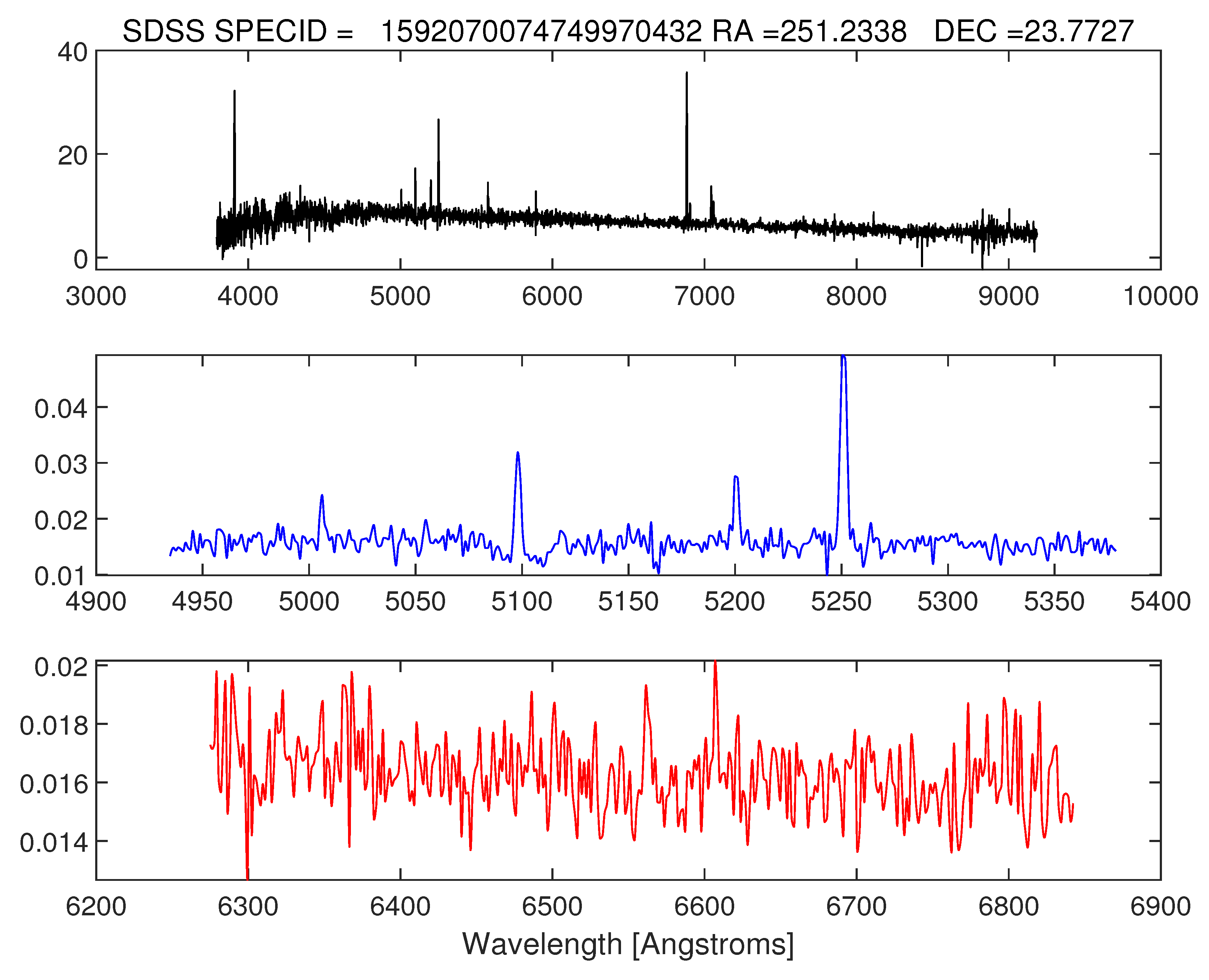
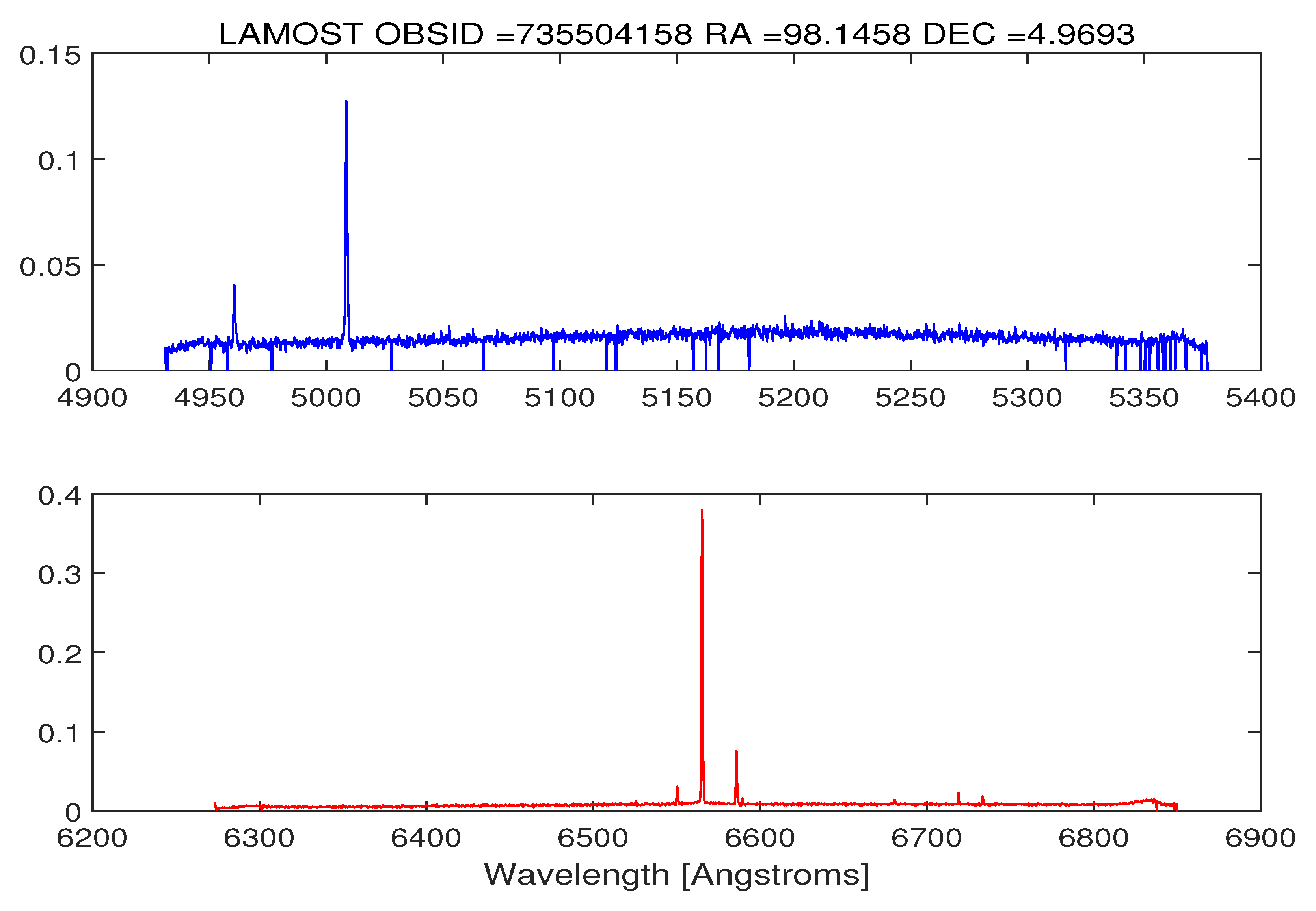
CVs are binary systems consisting of a white dwarf star and a companion star. The companion star is usually a K or M type red dwarf star, and in some cases a white dwarf star or a red giant star. CVs have important role and significance for studying the theory of accretion disks. Presently, only about two thousand CVs have been discovered [19]. Most of the optical spectra of CVs are identified by large surveys including SDSS [20,21,22,23,24], Far-Ultraviolet Spectroscopic Explorer (FUSE) [25], ROSAT XRT-PSPC All Sky Survey [26] and Catalina Real-time Transient Survey (CRTS) [27,28]. There are still some unresolved questions about CVs such as period gap due to the limitation of samples [29]. Higher requirements are put forward for new automatic classification methods for searching for CVs in massive spectra.

This paper is organized as follows. Section 2 describes experimental data and data preprocessing. We introduce the different methods used in the paper in Section 3. Section 4 presents the implementation of the methods in detail. Section 5 reports the results of our experiment. In Section 6, we give our conclusions and outline our plans for future work.

2. Data and Preprocessing

2.1. Positive Samples

Training samples especially positive samples are crucial to the classifier of machine learning. Because of the lack of previous identified CVs spectra of LAMOST, the training set is from SDSS whose spectra are homogeneous with LAMOST. SDSS has an authentic pipeline which has already classified the spectra into specified subclass. We can verify the proposed methods and construct a credible network with SDSS spectra and search for CVs in the unlabeled LAMOST spectra.

A total number of 417 1D spectra were selected from SDSS [30] as shown in Figure 1. Figure 2 is a MRS spectrum of LAMOST. The top and bottom panel are B (blue, 4950∼5350 Å) and R (red, 6300∼6800 Å) band respectively (all figures of LAMOST spectra follow the same rules). The SDSS spectra are trimmed within the same band of LAMOST in prepossessing.

2.2. Experimental Spectra for 1D Classification

46,180 1D M type spectra were selected from SDSS-DR16 for 1D spectral classification. 1234445 unlabeled 1D MRS spectra from LAMOST-DR7 are data source for CVs searching, as shown in the bottom of Figure 1.

2.3. Experimental Spectra for 2D Testing

LAMOST has overall 16 spectrographs and each spectrograph accommodates 250 fibers. The lights of 4000 celestial objects are fed into the fibers simultaneously and recorded on the CCD detectors after being transferred into the spectrographs. The 2D fiber spectral images of LAMOST are thus achieved. There are 250 2D fiber spectra in Figure 3 as shown from left to right and the wavelength increases from top to bottom. Figure 4 is a single 2D spectrum extracted from Figure 3. 2D spectra are normally used to produce the 1D spectra followed by post-processing steps.

For the lack of enough labeled 2D spectra from LAMOST, we fold the 1D SDSS spectrum into a spectral matrix for 2D processing.

2.4. Data Preprocessing

SDSS (R∼2000) and LAMOST (R∼7500) have different spectral resolutions and the two sets need to be brought at the same resolution, otherwise at their respective resolution, the spectrum of the same object from the two surveys will present different features. Their wavelength sampling and normalization are also carried out in data preprocessing.

The flux of spectra is interpolated as follows in data preprocessing:

$$y=\frac{(x-x_{i+1})(x-x_{i+2})}{(x_i-x_{i+1})(x_i-x_{i+2})}{y}_i+\frac{(x-x_i)(x-x_{i+2})}{(x_{i+1}-x_i)(x_{i+1}-x_{i+2})}{y}_{i+1}+\frac{(x-x_i)(x-x_i)}{(x_{i+2}-x_i)(x_{i+2}-x_{i+1})}{y}_{i+2}$$

(1)

Using the method above, the spectra with ∼4000 flux values (features) are interpolated to 5000 dimensions and folded into a m * n spectral matrix for 2D processing. In our experiment, m = 50 and n = 100 are empirical values.

SNR and spectral type are two important factors influencing the classification. M type stars from SDSS are selected for their influence analysis in the experiment. The distribution of M type spectra is shown in Figure 5.

The spectra are classified according to the SNR and the type of M stars of SDSS. The SNR is divided into 5∼10, 10∼15, and above 15 and the type M stars are divided into five subclasses from M0∼M4. The specific spectra are shown in Figure 6.

3. Methods

The goal of spectra classification is to maximize common features and minimize noise and spectral individual features. A variety of classification networks are employed and tested.

3.1. Convolutional Neural Network

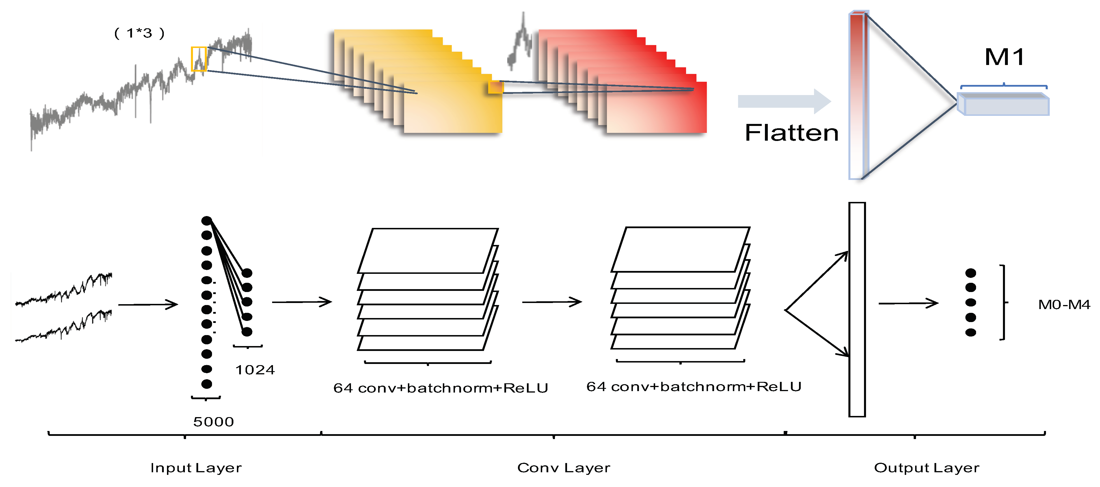
CNN can handle both 1D and 2D data, depending on whether its kernel is 1D or 2D. We use CNN to classify M stars, because CNN performs well in image classification, and it can also handle 1D spectra classification. The feature extraction capabilities of CNN can help us to improve the accuracy of traditional classification methods. Quadratic interpolation is performed to facilitate the folding of the spectra to form a 2D spectral matrix.

As a special form of CNN, 1D CNN has certain applications in the field of signal processing. We adopted the network structure shown in Figure 7.

In the specific network construction, the backpropagation algorithm is adopted. The 1D matrix information composed of spectra is continuously trained to fit the parameters in each layer by gradient descent.

Using the total errors to calculate the partial derivative of the parameter, the magnitude of the influence of a parameter on the overall errors can be obtained, which is used to correct the parameters in the back propagation. Since the construction of the network uses a linear arrangement, the total error calculated by the final output layer is used to perform the partial derivative calculation of the parameters in all layers:

$$\frac{\partial E}{\partial W_{x_j}}=\frac{\partial E}{\partial Ou{t}_n}\ast \frac{\partial Ou{t}_n}{\partial Ne{t}_n}\ast \cdots \cdots \ast \frac{\partial Ou{t}_x}{\partial Ne{t}_x}\ast \frac{\partial Ne{t}_x}{\partial w_{x_j}}$$

(2)

Each neuron in a CNN network is connected to all neurons in the previous layer, so the calculation of the local gradient requires a forward recursive calculation of the gradient of each subsequent layer of neurons. After defining the linear output of each layer and the parameters in the structure, the output of the activation function is: $Out=\phi \left(v\right)$, then the recursive formula for each gradient can be derived as:

$${\delta }_{ij}^{l-1}=\frac{\partial E}{\partial V_{ij}^{l-1}}=\frac{\partial E}{\partial Ou{t}_{ij}^{l-1}}\ast \frac{\partial Ou{t}_{ij}^{l-1}}{\partial V_{ij}^{l-1}}=\frac{\partial E}{\partial Ou{t}_{ij}^{l-1}}\ast {\phi }^{\prime }\left(V_{ij}^{l-1}\right)$$

(3)

In the successive calculation of the formula above, the gradient calculated by each parameter under the total errors is used as the basis to achieve the goal of correcting the parameters in the direction of the minimum loss function.

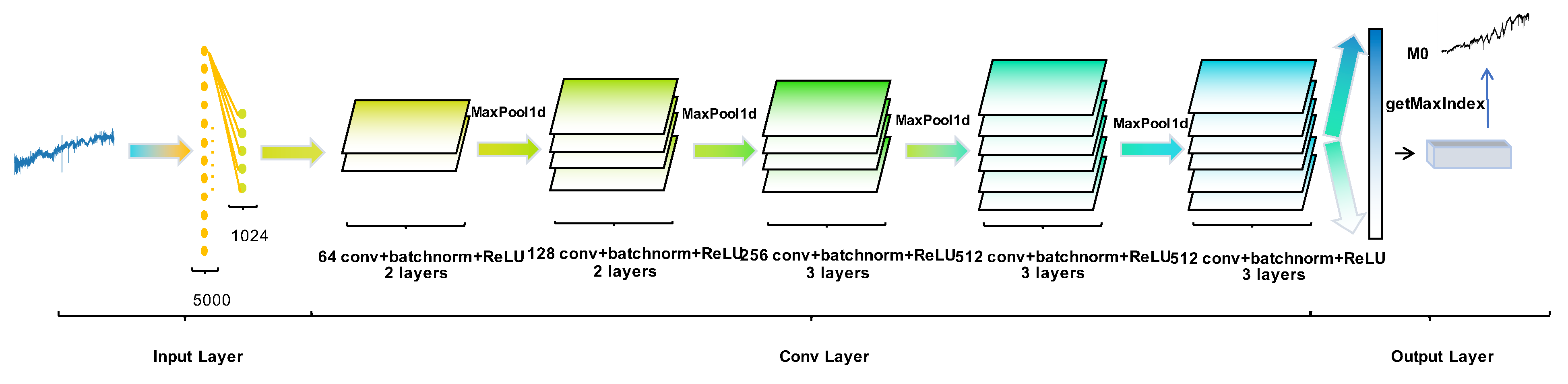
3.2. VGGNet and ResNet

VGGNet with prominent generalization ability for different datasets is widely used in 2D data processing. Considering that our spectral dimensions are not particularly large, in order to prevent overfitting on the training set, the shallow VGG16 network shown in Figure 8 is used in our experiments.

The greatest improvement of VGGNet is to convert large and short convolutional layers into small and deep neural networks by reducing the scale of convolution kernels. In the convolutional layer, the number of extracted features for each layer output can be calculated using the following formula:

$$n_{out}=\left(\frac{n_{in}+2p-k}{s}\right)+1$$

(4)

p, k and s are the size of max pooling, kernel size, and stride, respectively. With the continuous development of the classification network, the network is constantly deepening for better extraction and feature combination, but the deep network makes it difficult to train and has a potential of losing information.

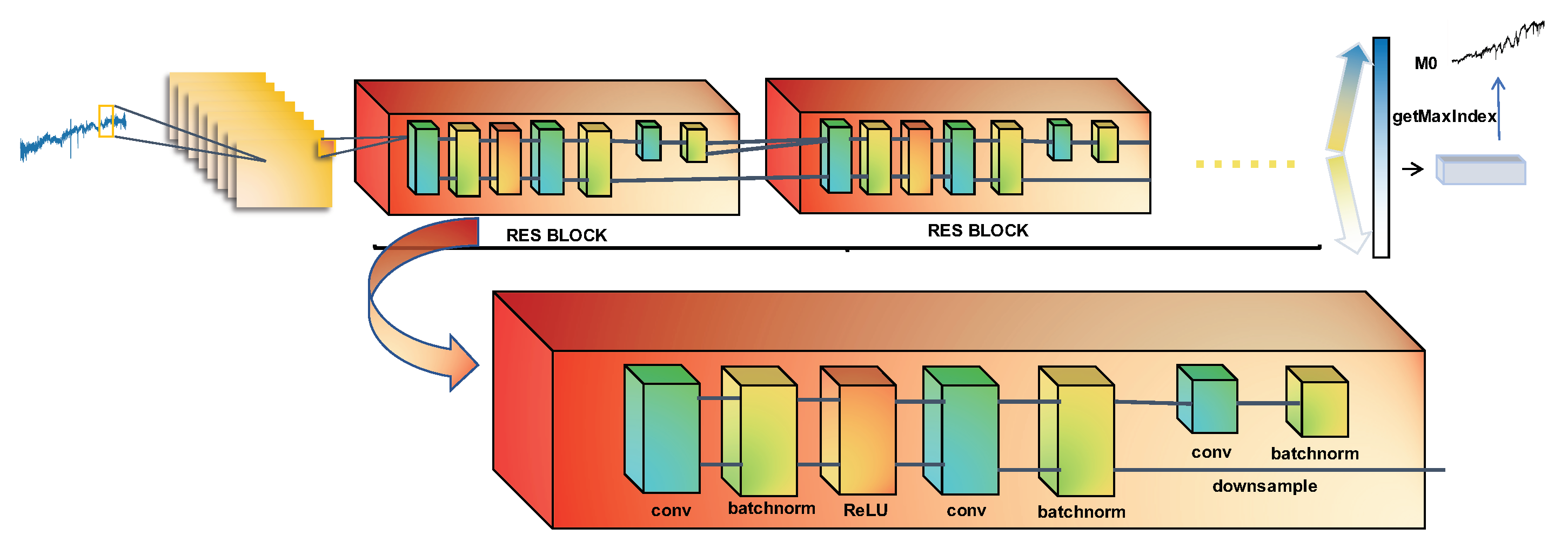
ResNet as shown in Figure 9 proposes residual learning to solve these problems, allowing information to be transmitted over the layer to preserve information integrity, while learning only the residuals of the previous network output:

$$F\left(x\right):=H\left(x\right)-x$$

(5)

This allows us to increase the number of convolutional layers, which is an effective way to train a very deep network. The most prominent characteristic of ResNet is that in addition to the result of the conventional convolution calculation in the final output, the initial input value is also added. Therefore, the result of network fitting will be the difference between the two, thereby we can obtain the calculation formula of each layer of ResNet as follows:

$$\begin{array}{c}\hfill Ou{t}^l=\phi (z^l+Ou{t}^{l-1})=\phi (w^l\ast Ou{t}^{l-1}+b^l+Ou{t}^{l-1})=\\ \hfill \phi [(w^l+1)\ast Ou{t}^{l-1}+b^l]\end{array}$$

(6)

Then the gradient calculation formula of the neural network is changed based on conventional ones:

$${\delta }_{ij}^{l-1}=\frac{\partial E}{\partial Ou{t}_{ij}^{l-1}}\ast [1+{\phi }^{\prime }\left(v_{ij}^{l-1}\right)]$$

(7)

Compared with the traditional networks, the extra value “1” makes the calculated gradient value difficult to disappear, which means that the gradient calculated from the last layer can be transmitted back in the reverse direction, and the effective transmission of the gradient makes spectral features more efficient in the training of neural networks. However, considering that our spectral features are limited and may have high noise interference, the efficient feature extraction of the network may lead to significant overfitting, which makes the trained network generalization capability poor.

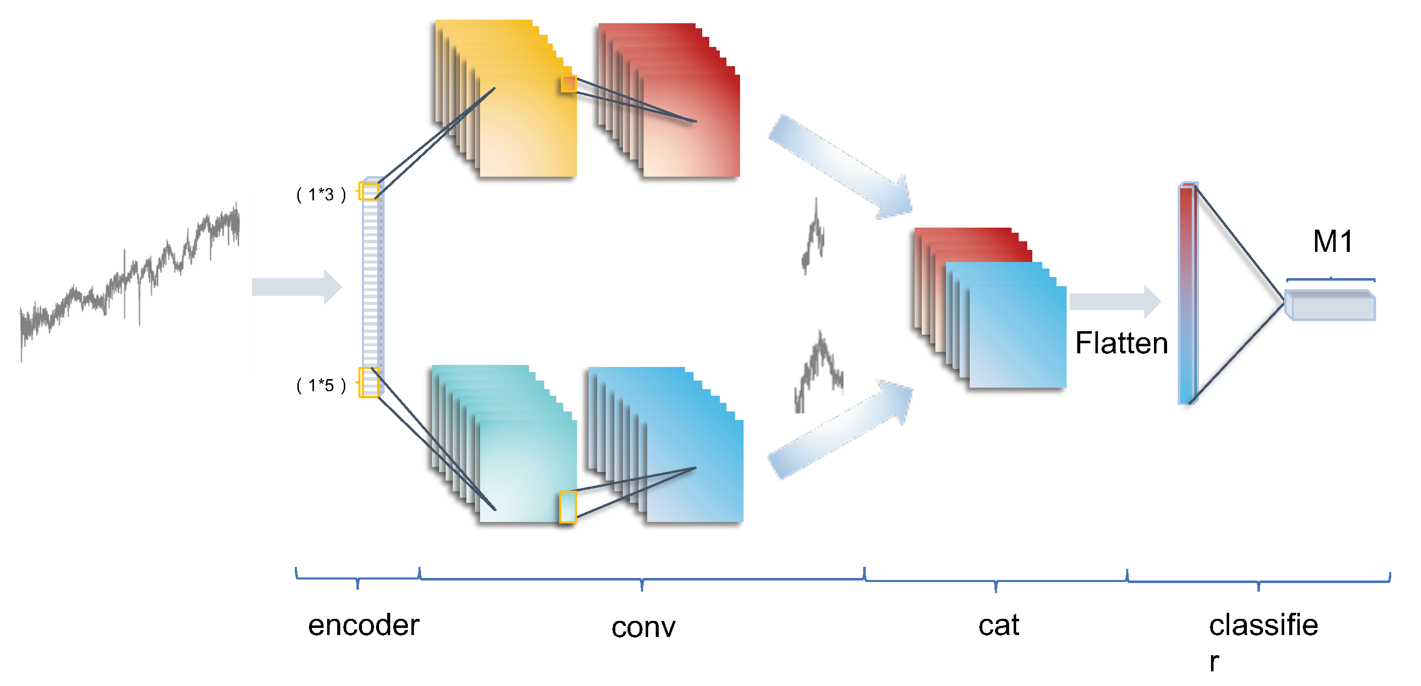
3.3. EMCCNN

EMCCNN is a network designed for the characteristics of spectra, and has achieved good results for different SNR spectra. We find that for spectra, a deep convolutional layer can lead to significant overfitting of the data and a very poor generalization capability of the model. Direct convolution of spectra will extract a lot of noise and individual features, which is not an ideal way to classify spectra. Unsupervised denoising methods tend to remove some spectral feature peaks in the data, which is also not an ideal method to maximize the common features of this spectral type.

Therefore, we try to add a supervised denoising network before the convolutional neural network, which can help in the identification of features and noise. It allows the network to extract spectral features instead of noise. On the other hand, the spectral feature peak types are not consistent. For different types of feature peaks, the different convolution kernel sizes may be able to extract different quality features. The extraction of some features may be better for larger convolution kernels. Others may be more friendly for small-scale convolution kernels. We decided to let convolution kernels of different scales learn features simultaneously, then combine these features, and obtain different weights for features through the fully connected layer. A better feature extraction network EMCCNN can be obtained as shown in Figure 10. The detailed description for the architecture of EMCCNN is shown in Appendix A and we use cross-entropy loss as loss function of EMCCNN.

4. Experiment

4.1. 1D Convolution Experiment and Results

The massive LAMOST spectra in this experiment are unlabeled, in order to verify the validity and efficiency of the method, we applied it in SDSS spectra before searching for CVs in massive LAMOST spectra.

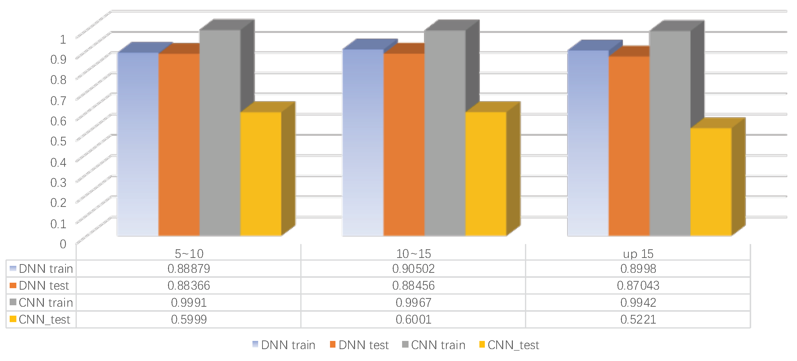
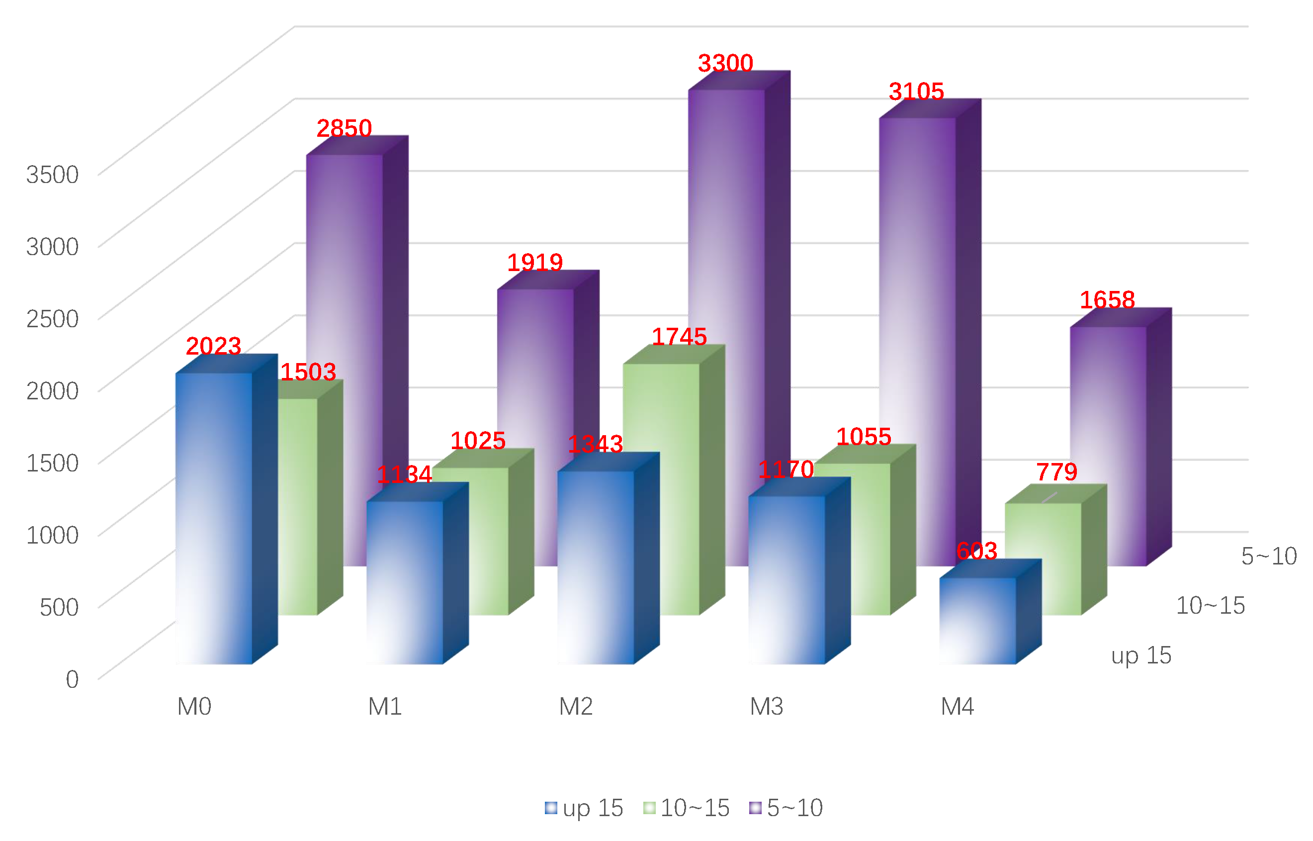
We first try to compare the spectra classification of DNN (Deep Neural Network) with four hidden layers and 1D CNN as shown in Figure 11. The optimizer used was a random gradient descent, the learning rate was set to ${10}^{-4}$, and the activation function chosen was ReLU (Rectified Linear units). We found that the CNN network can quickly extract the corresponding features, but it will also overfit quickly, which has an accuracy (number of spectra correctly classified to the parent class/number of total spectra) of 60% in the test set, and the generalization capability is extremely poor.

CNN has strong feature extraction capabilities, but it is not suitable for spectra because it also extracts quite a lot of individual features and noise simultaneously. The problem becomes even worse with the increment of SNR.

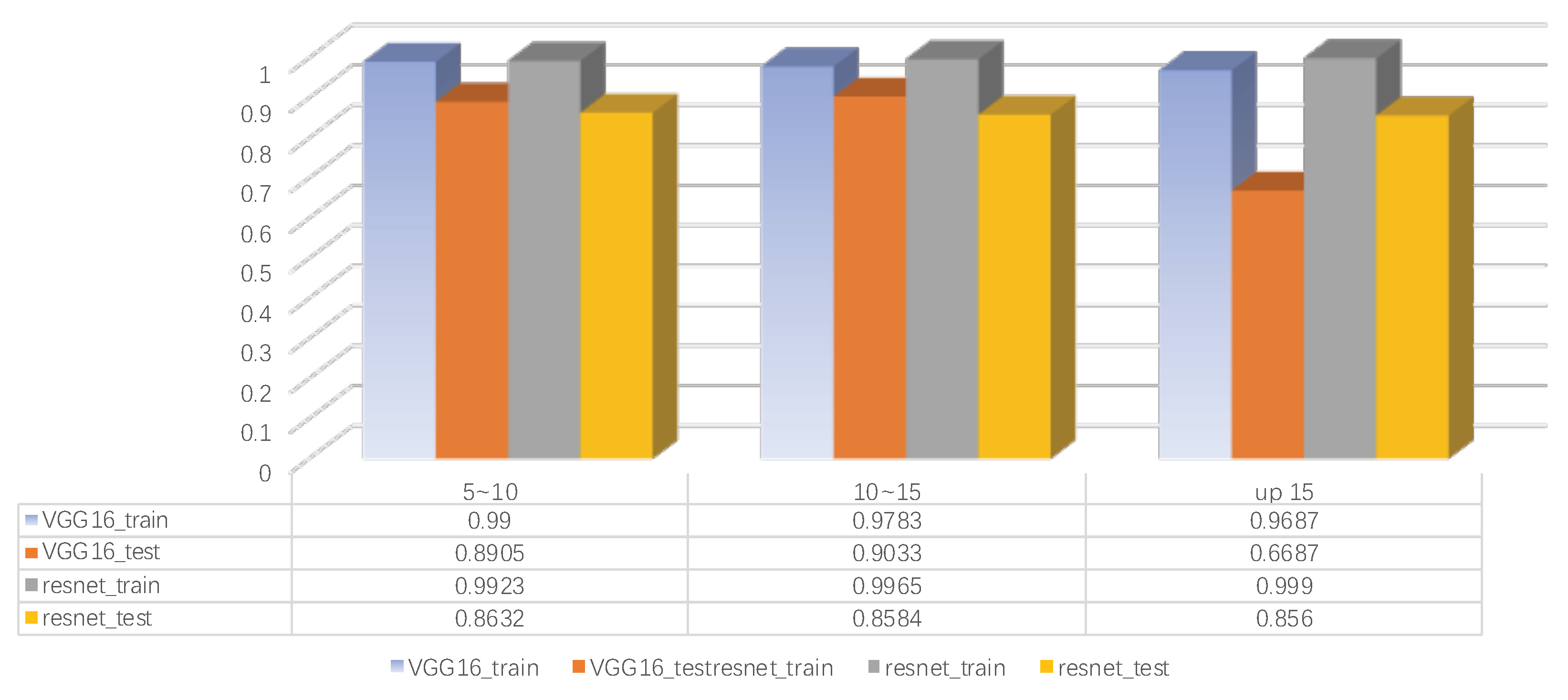
Considering that VGG16 is composed of several convolutional layers, the direct convolution of the spectra will be the same as the direct use of CNN, leading to the overfitting of the training data. Hence, we try to add the encoder to the VGG16 network to denoise. We found that after denoising, VGG16 is not as bad as CNN for spectra within the scope of $5\le sn\le 15$, but it is also not satisfactory for spectra with $sn$ > 15. It is considered that the data features of high SNR are more obvious. The spectral individual features and noise will have a strong interference effect on a very deep network. On the other hand, the feedback process of the denoising encoder is too long, which is not easy to identify the difference of individual features, noise and common features.

ResNet’s interlayer transfer mechanism might help us solve the problem of overfitting, but the effect is not very satisfactory. ResNet and CNN also perform well on the training data, and can reach more than 99% accuracy on the three SNRs. It does not perform well in the test set, although not as serious as CNN. We try to add the dropout layer to help us solve the problem of overfitting, but this makes our training very slow and the final result is not satisfactory as well, as shown in Figure 12.

Through experiments shown in

Table 1. 1D classification accuracy of different network models.

	SN	5–10		10–15		up15
Model
		train	test	train	test	train	test
DNN		0.8888	0.8837	0.9050	0.8846	0.8998	0.8704
CNN		0.9991	0.5999	0.9967	0.6001	0.9942	0.5221
VGG16		0.9900	0.8905	0.9783	0.9033	0.9687	0.6687
ResNet		0.9923	0.8632	0.9965	0.8584	0.9990	0.8560
EMCCNN		0.9813	0.9206	0.9897	0.9223	0.9461	0.8962

, it is noticed that the network with deep structure is not suitable for the classification of spectra, which will make the individualized features of noise and spectrum fully extracted, and the denoising of the encoder before these networks will make the feedback time too long, leading to a bad denoising result. Based on the conclusions above, we propose EMCCNN, which is not too deep, and is beneficial to the training of denoising capability of the encoder. We find that EMCCNN is very robust to SNR, which is especially suited for the spectra of LAMOST.

For objective comparison, we used support vector machine (SVM) to directly process spectra for classification and compare with the results of EMCCNN in

Table 2. Classification accuracy of different network models.

	SN	5–10		10–15		up15
Model
		train	test	train	test	train	test
SVM		1	0.6802	1	0.7213	1	0.741
EMCCNN		0.9813	0.9206	0.9897	0.9223	0.9461	0.8962

. The comparison demonstrates that SVM can quickly fit the training set of the data, but it tends to overfit critically in the experiment.

4.2. 2D Convolution Experiment and Results

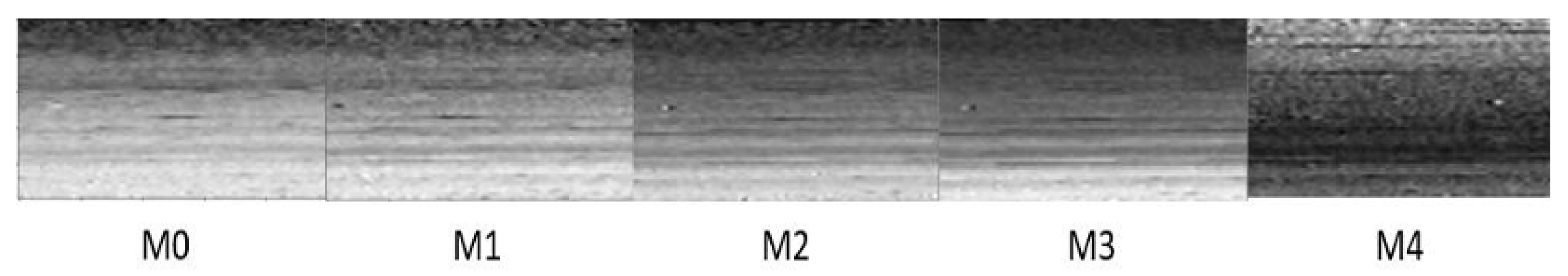
We apply the classification network that is currently applied to 2D data in the field of spectra classification to explore the classification feasibility of the 2D folding of the 1D data. We fold the spectra into a 50 × 100 matrix and put it into a 2D classification network for experiments. The feature peaks of spectra become inconspicuous after folding. The spectra are only related on the same line after folding. The data correlation for each column is not obvious, but from the picture we can clearly see that each type of spectra is different after folding in Figure 13, which brings us the possibility of applying the 2D classification network. We aim to fully apply the classification network so that satisfactory performance can be achieved.

AS shown in

Table 3. Classification accuracy of different network models (1D and 2D).

	SN	5–10		10–15		up15
Model
		train	test	train	test	train	test
CNN_1d		0.9991	0.5999	0.9967	0.6001	0.9942	0.5221
CNN_2d		0.9971	0.8288	0.9977	0.8271	0.9980	0.7310
VGG16_1d		0.9900	0.8905	0.9783	0.9033	0.9687	0.6687
VGG16_2d		0.9846	0.9103	0.9722	0.9320	0.9900	0.8504
ResNet_1d		0.9923	0.8632	0.9965	0.8584	0.9990	0.8560
ResNet_2d		0.9949	0.8738	0.9977	0.8801	0.9938	0.8132
EMCCNN_1d		0.9813	0.9206	0.9897	0.9223	0.9461	0.8962
EMCCNN_2d		0.9986	0.8956	0.9940	0.9049	0.9906	0.8835

, VGG16 performs quite well in the range of 10 < sn < 15 SNR, and ResNet also performs better than 1D spectra in the range of 5 < sn < 15. This discovery is inspiring, because it proves that although 1D spectra is not directly related to the top and bottom after folding, the 2D classification network can still achieve satisfactory results, which proves that the 2D classification of 1D spectra is feasible, even for some spectra which can produce results better than 1D classification.

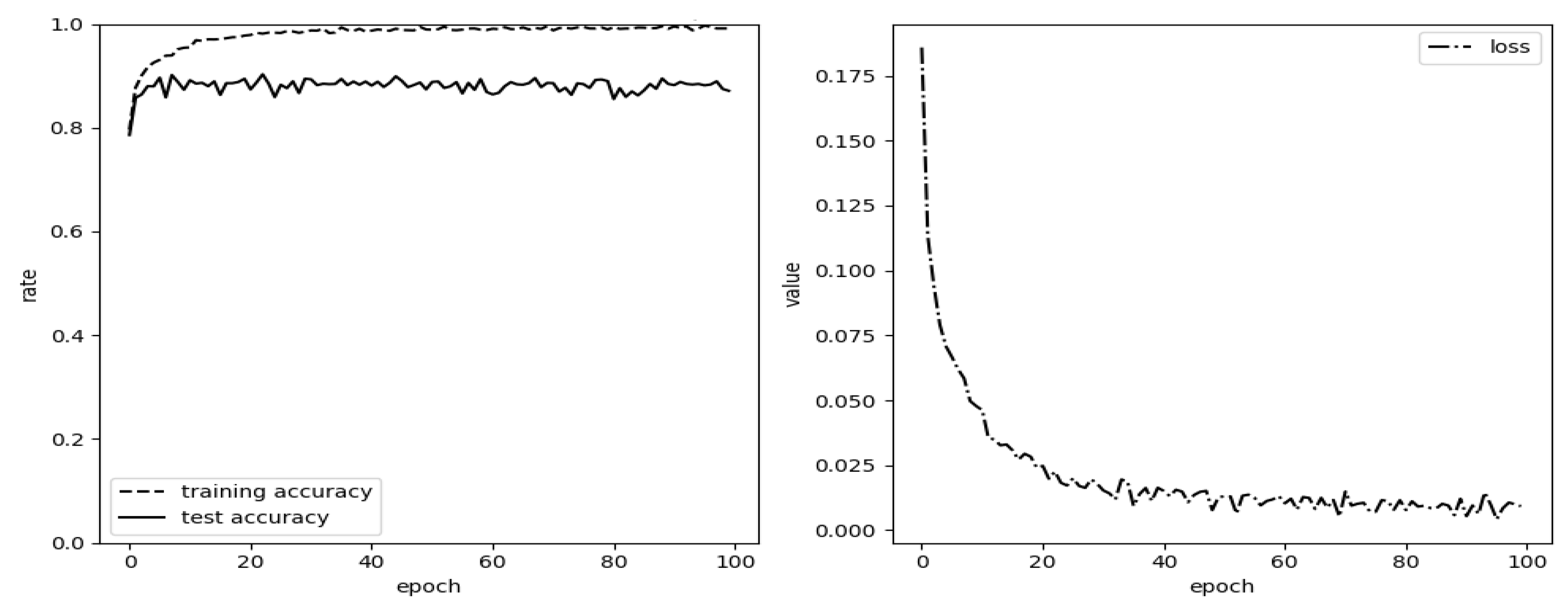
Because the results of ResNet_2d on the training set are very good, we try to use early stopping to overcome overfitting. We show the results of ResNet_2d at different epochs in Figure 14. Obviously early stopping cannot improve the accuracy in test set.

After the above comprehensive analysis and comparison of the methods under different situations, EMCCNN shows its superiority in 1D spectra especially its robustness against noise and is selected as the final structure to search for CVs in LAMOST archives.

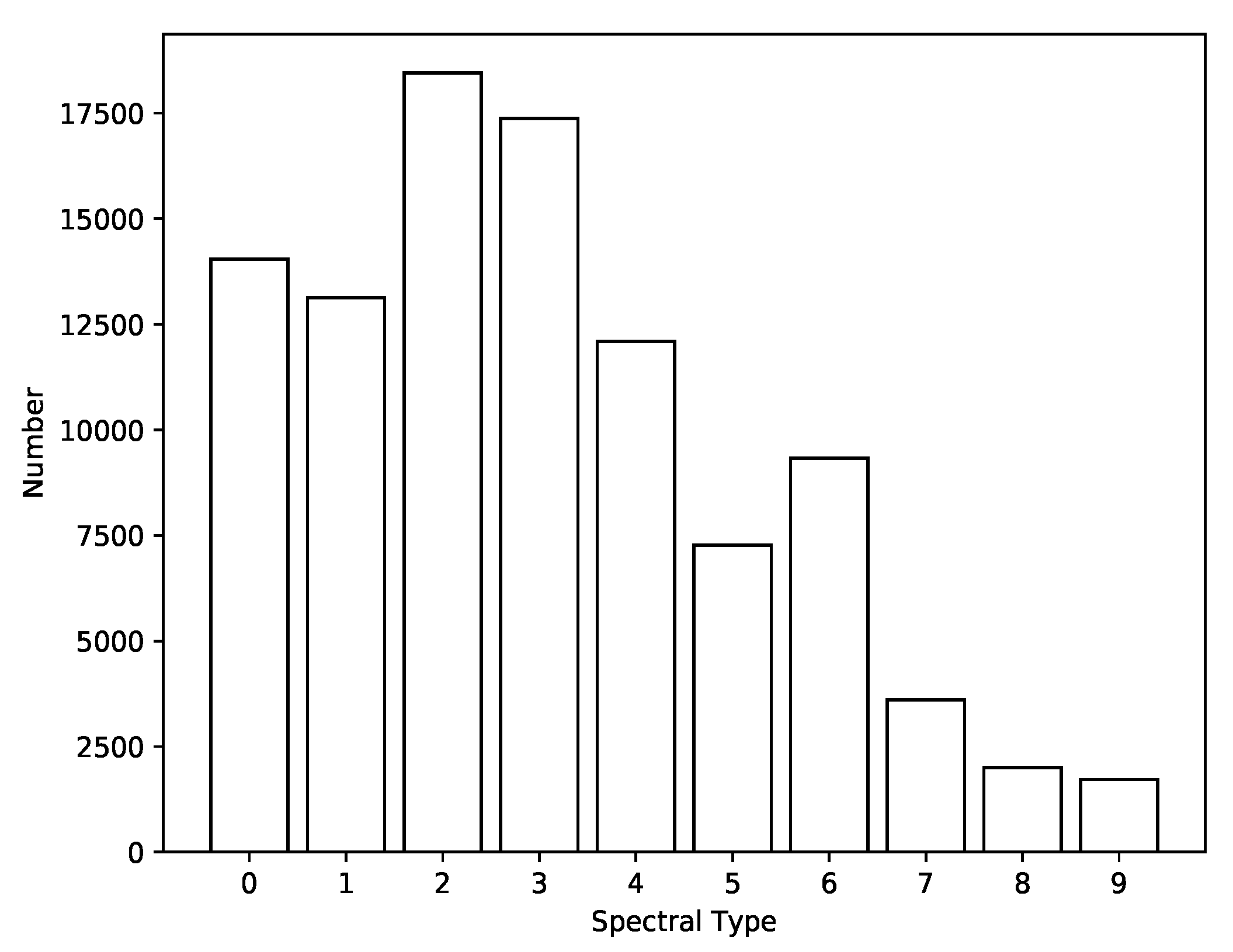
4.3. Subclass Classification Results

Because the experimental spectra categories are not uniform, we explore the detailed results of the spectral categories in this section. Here we use $precision\left(P\right)$, $recall\left(R\right)$ and $F\text{-}measure\left(F\right)$ to judge the performance of EMCCNN for each subclass.

$$precision=\frac{TP}{TP+FP}$$

(8)

$$recall=\frac{TP}{TP+FN}$$

(9)

$$F\text{-}measure=\frac{2·precision·recall}{precision+recall}$$

(10)

where $TP$ are current subclass samples predicted correctly by classifier and $FP$ are other subclass samples which is wrongly predicted to current subclass. $FN$ are current subclass samples wrongly predicted to other subclass samples.

Because the subclass data is not uniform and the number of features is not consistent, the performance of the EMCCNN in each subclass is not the same. We show results in

Table 4. Fine Classification Results of EMCCNN.

	SN	5–10			10–15			up15
Model
		P	R	F	P	R	F	P	R	F
EMCCNN_1d m0		0.9336	0.7699	0.8439	0.9392	0.7840	0.8546	0.9197	0.8036	0.8577
EMCCNN_1d m1		0.9312	0.6448	0.7620	0.9050	0.6908	0.7835	0.8807	0.6421	0.7427
EMCCNN_1d m2		0.7190	0.5631	0.6315	0.6992	0.6078	0.6503	0.5068	0.2761	0.3574
EMCCNN_1d m3		0.9360	0.7655	0.8422	0.9590	0.6381	0.7663	0.9068	0.6187	0.7355
EMCCNN_1d m4		0.8991	0.6500	0.7545	0.9074	0.6336	0.7461	0.8606	0.4751	0.6122
EMCCNN_2d m0		0.9404	0.7093	0.8087	0.9276	0.7682	0.8404	0.9655	0.7509	0.8448
EMCCNN_2d m1		0.8555	0.6097	0.7120	0.8958	0.6515	0.7543	0.8240	0.6508	0.7272
EMCCNN_2d m2		0.7218	0.5394	0.6174	0.7857	0.6620	0.7185	0.6194	0.4093	0.4929
EMCCNN_2d m3		0.9034	0.7389	0.8129	0.8756	0.6692	0.7586	0.8481	0.6504	0.7362
EMCCNN_2d m4		0.9121	0.5722	0.7032	0.9655	0.5668	0.7142	0.9107	0.4322	0.5862

.

5. Results of CVs Searching in LAMOST Spectra

A systematic search for CVs in MRS of LAMOST is carried out with EMCCNN. After cross-matching the results of EMCCNN with Simbad2, 15 spectra are identified by EMCCNN as CVs, of which one is a CV candidate observed three times. In

Table 5. Known and possible CVs identified by the method.

OBSID ${}^1$	RA (J20000) ${}^2$	Dec (J2000) ${}^3$	GALLONG ${}^4$	GAL_LAT ${}^5$	Type ${}^6$	GCVS Name ${}^7$	Refs ${}^8$
691006174	119.684	12.0315	209.4821	20.3034	CVs		1
692108157	132.6541	11.9013	215.5055	31.7867	CVs		2∼6
682303114	84.2381	0.35996	203.8671	−16.3386	CVs		7∼10
715907098	206.2679	0.71487	331.1331	60.6159	CVs	AA Vir	11∼12
737803139	129.5916	48.6339	170.8817	37.3575	Dwarf Nova	EI UMa	13∼17
690602249	333.9029	55.6329	102.1415	−0.81833	Nova	CP Lac	18∼22
693002098	30.453	56.7182	132.5141	−4.8385	Nova	V Per	23∼27
727705022	82.1711	33.3113	174.364	−0.70689	Nova	QZ Aur	26∼30
728005022	82.1703	33.3176	174.3584	−0.70401	Nova	QZ Aur	28∼32
728605022	82.1626	33.3125	174.3591	−0.7122	Nova	QZ Aur	28∼32
729105022	82.1711	33.3113	174.364	−0.70689	Nova	QZ Aur	28∼32
729205022	82.1711	33.3113	174.364	−0.70689	Nova	QZ Aur	28∼32
681816126	306.8251	42.7639	80.7472	2.5337	CVs Candidate		33
682416126	306.8251	42.7639	80.7472	2.5337	CVs Candidate		33
683116126	306.8251	42.7639	80.7472	2.5337	CVs Candidate		33

${}^1$ OBSID = Unique number ID of this spectrum in LAMOST. ${}^2$ RA = Right Ascension (J2000). ${}^3$ Dec = Declination (J2000). ${}^4$ GAL_LONG = Galactic longitude. ${}^5$ GAL_LAT = Galactic latitude. ${}^6$ Simbad name. ${}^7$ GCVS (General Catalog of Variables) name. ${}^8$ Representative references to discovery papers—(1) Carter et al. [31]; (2) Gaia Collaboration et al. [32]; (3) Nardiello et al. [33]; (4) Geller et al. [34]; (5) Mooley and Singh [35]; (6) Pineau et al. [36]; (7) Gentile Fusillo et al. [37]; (8) Kleinman et al. [38]; (9) Thorstensen and Skinner [39]; (10) Szkody et al. [40]; (11) Drake et al. [41]; (12) Palaversa et al. [42]; (13) Suleimanov et al. [43]; (14) Schwope [44]; (15) Mukai [45]; (16) Pretorius and Mukai [46]; (17) Baumgartner et al. [47]; (18) Selvelli and Gilmozzi [48]; (19) Shara et al. [49]; (20) Özdönmez et al. [50]; (21) Vogt et al. [51]; (22) Schaefer [52]; (23) Sahman et al. [53]; (24) Pagnotta and Schaefer [54]; (25) Scaringi [55]; (26) Harrison et al. [56]; (27) Tappert et al. [57]; (28) Schaefer et al. [58]; (29) Shi and Qian [59]; (30) Schaefer [52]; (31) Shafter [60]; (32) Salazar et al. [61]; (33) Verbeek et al. [62].

, the identified CVs are listed with RA, GCVS names, type etc. Their spectra are shown from Figure 15, Figure 16, Figure 17 and Figure 18. We report the spectra in the website https://github.com/whkunyushan/CVs.

6. Conclusions

There is a great need for accurate and automatic classification methods of specified objects in massive spectra. The goal that we propose for spectral feature extraction is to maximize the extraction of common features and to minimize the extraction of noise and spectral individual features, which enhances the generalization capabilities of the network. We found that the simple DNN network cannot extract the features of spectra well, but the CNN with strong feature extraction capability can lead to significant overfitting. It also emerges that the deep network is not suited for the denoising training of the encoder, because its feedback process can be very long. This makes the encoder difficult to train and achieve a good denoising result.

In most cases, CVs especially CVs at quiescence show emission lines of Balmer series, HeI and HeII lines. For LAMOST spectra, only the H$\alpha$ emission line (6563 Å) is included in B band which gives it a higher request for the ability of this feature extraction method. In this work, EMCCNN simultaneously performs supervised denoising, feature extraction, and classification. EMCCNN is not a deep network, which is ideal for the encoder to achieve a good denoising result. On the other hand, convolution kernels of different scales can extract spectral peaks of different quality, which provides sufficient options for the classifier. By weighting up the quality of features, the network can select high-quality spectral type features. This design enables the EMCCNN to achieve the best results in the three SNRs of 1D data.

The traditional view is that folding a 1D spectrum into a 2D image causes an information loss and the network has to do extra learning to understand that the pixels are correlated only along the horizontal axis and not along the vertical axis. However, EMCCNN achieve precise acquisition of the characteristic features of folded 2D spectra and can achieve good classification results, especially in the case where the 1D classification tends to overfit to an extreme degree. It proves that folding the spectra into 2D can effectively prevent the tendency of overfitting under certain circumstances.

Furthermore, this paper creatively proves that the classification of 2D spectra is feasible which means as a method of deep learning, powerful deep learning SDK (Software Development Kit) such as Caffe, Cognitive toolkit, PyTorch, TensorFlow, etc. and image processing libraries can be used for 2D spectral classification directly.

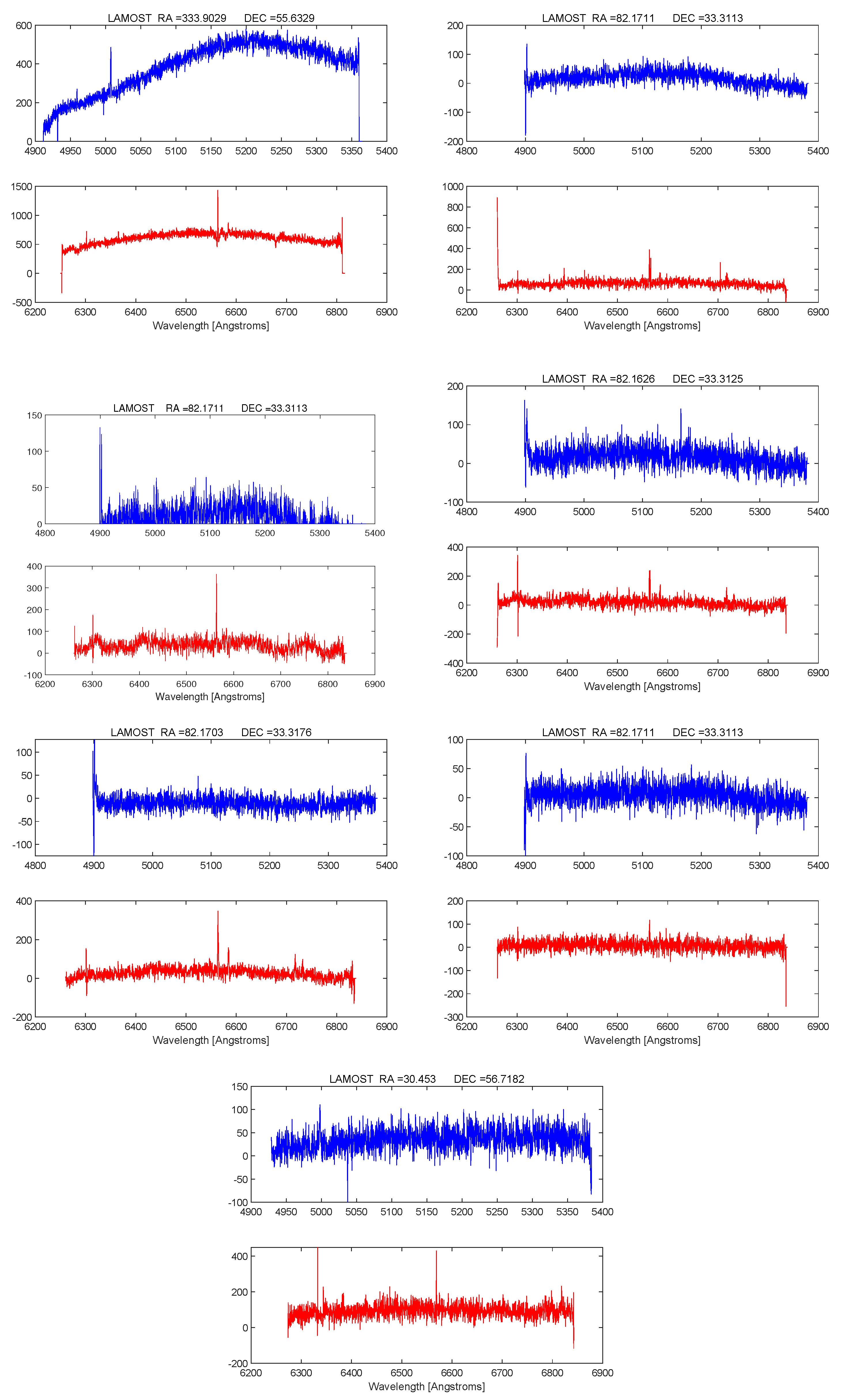
The discovery of the MRS of LAMOST provide more samples for astronomers to characterize the population of CVs. More new CVs will be discovered with the gradual release of LAMOST spectra.

References

1. Yanny, B.; Rockosi, C.; Newberg, H.J.; Knapp, G.R.; Adelman-McCarthy, J.K.; Alcorn, B.; Allam, S.; Allende Prieto, C.; An, D.; Anderson, K.S.J.; et al. SEGUE: A Spectroscopic Survey of 240,000 Stars with g = 14–20. Astron. J. 2009, 137, 4377–4399. [Google Scholar] [CrossRef] [Green Version]
2. Blanton, M.R.; Bershady, M.A.; Abolfathi, B.; Albareti, F.D.; Allende Prieto, C.; Almeida, A.; Alonso-García, J.; Anders, F.; Anderson, S.F.; Andrews, B.; et al. Sloan Digital Sky Survey IV: Mapping the Milky Way, Nearby Galaxies, and the Distant Universe. Astron. J. 2017, 154, 28. [Google Scholar] [CrossRef]
3. Cui, X.Q.; Zhao, Y.H.; Chu, Y.Q.; Li, G.P.; Li, Q.; Zhang, L.P.; Su, H.J.; Yao, Z.Q.; Wang, Y.N.; Xing, X.Z.; et al. The Large Sky Area Multi-Object Fiber Spectroscopic Telescope (LAMOST). Res. Astron. Astrophys. 2012, 12, 1197–1242. [Google Scholar] [CrossRef]
4. Zhao, G.; Zhao, Y.H.; Chu, Y.Q.; Jing, Y.P.; Deng, L.C. LAMOST spectral survey—An overview. Res. Astron. Astrophys. 2012, 12, 723–734. [Google Scholar] [CrossRef]
5. Lei, Z.; Zhao, J.; Németh, P.; Zhao, G. Hot Subdwarf Stars Identified in Gaia DR2 with Spectra of LAMOST DR6 and DR7. I. Single-lined Spectra. Astrophys. J. 2020, 889, 117. [Google Scholar] [CrossRef] [Green Version]
6. Warner, B. Cataclysmic Variable Stars; Cambridge Astrophysics Series; Cambridge University Press: Cambridge, UK, 1995; Volume 28. [Google Scholar]
7. Worraker, B. Book Review: Cataclysmic Variable Stars: How and why they vary (Coel Hellier). Astronomer 2001, 38, 47–48. [Google Scholar]
8. Gänsicke, B.T.; Dillon, M.; Southworth, J.; Thorstensen, J.R.; Rodríguez-Gil, P.; Aungwerojwit, A.; Marsh, T.R.; Szkody, P.; Barros, S.C.C.; Casares, J.; et al. SDSS unveils a population of intrinsically faint cataclysmic variables at the minimum orbital period. Mon. Not. R. Astron. Soc. 2009, 397, 2170–2188. [Google Scholar] [CrossRef]
9. Baron, D.; Poznanski, D.; Watson, D.; Yao, Y.; Cox, N.L.J.; Prochaska, J.X. Using Machine Learning to classify the diffuse interstellar bands. Mon. Not. R. Astron. Soc. 2015, 451, 332–352. [Google Scholar] [CrossRef] [Green Version]
10. Banerji, M.; Lahav, O.; Lintott, C.J.; Abdalla, F.B.; Schawinski, K.; Bamford, S.P.; Andreescu, D.; Murray, P.; Raddick, M.J.; Slosar, A.; et al. Galaxy Zoo: Reproducing galaxy morphologies via machine learning. Mon. Not. R. Astron. Soc. 2010, 406, 342–353. [Google Scholar] [CrossRef] [Green Version]
11. Ball, N.M.; Brunner, R.J.; Myers, A.D.; Strand, N.E.; Alberts, S.L.; Tcheng, D. Robust Machine Learning Applied to Astronomical Data Sets. III. Probabilistic Photometric Redshifts for Galaxies and Quasars in the SDSS and GALEX. Astrophys. J. 2008, 683, 12–21. [Google Scholar] [CrossRef] [Green Version]
12. Gural, P.S. Deep learning algorithms applied to the classification of video meteor detections. Mon. Not. R. Astron. Soc. 2019, 489, 5109–5118. [Google Scholar] [CrossRef]
13. Sharma, K.; Kembhavi, A.; Kembhavi, A.; Sivarani, T.; Abraham, S.; Vaghmare, K. Application of convolutional neural networks for stellar spectral classification. Mon. Not. R. Astron. Soc. 2020, 491, 2280–2300. [Google Scholar] [CrossRef]
14. Liu, K.; Zhong, P.; Zheng, Y.; Yang, K.; Liu, M. P_VggNet: A convolutional neural network (CNN) with pixel-based attention map. PLoS ONE 2018, 13, e0208497. [Google Scholar] [CrossRef] [PubMed]
15. He, K.; Zhang, X.; Ren, S.; Sun, J. Identity Mappings in Deep Residual Networks; Computer Vision—ECCV 2016; Leibe, B., Matas, J., Sebe, N., Welling, M., Eds.; Springer International Publishing: Cham, Switzerland, 2016; pp. 630–645. [Google Scholar]
16. Tao, Y.; Xu, M.; Lu, Z.; Zhong, Y. DenseNet-Based Depth-Width Double Reinforced Deep Learning Neural Network for High-Resolution Remote Sensing Image Per-Pixel Classification. Remote Sens. 2018, 10, 779. [Google Scholar] [CrossRef] [Green Version]
17. Hála, P. Spectral classification using convolutional neural networks. arXiv 2014, arXiv:1412.8341. [Google Scholar]
18. Corral, L.; Navarro, S.G.; Villavicencio, E. Effect of the Signal to Noise Ratio on the Accuracy of the Automatic Spectral Classification of Stellar Spectra. In Astronomical Data Analysis Software and Systems XXVI; Astronomical Society of the Pacific Conference Series; Molinaro, M., Shortridge, K., Pasian, F., Eds.; Astronomical Society of the Pacific: San Francisco, CA, USA, 2019; Volume 521, p. 351. [Google Scholar]
19. Samus, N.N.; Kazarovets, E.V.; Durlevich, O.V.; Kireeva, N.N.; Pastukhova, E.N. General catalogue of variable stars: Version GCVS 5.1. Astron. Rep. 2017, 61, 80–88. [Google Scholar] [CrossRef]
20. Szkody, P.; Anderson, S.F.; Agüeros, M.; Covarrubias, R.; Bentz, M.; Hawley, S.; Margon, B.; Voges, W.; Henden, A.; Knapp, G.R.; et al. Cataclysmic Variables from The Sloan Digital Sky Survey. I. The First Results. Astron. J. 2002, 123, 430–442. [Google Scholar] [CrossRef]
21. Szkody, P.; Fraser, O.; Silvestri, N.; Henden, A.; Anderson, S.F.; Frith, J.; Lawton, B.; Owens, E.; Raymond, S.; Schmidt, G.; et al. Cataclysmic Variables from the Sloan Digital Sky Survey. II. The Second Year. Astron. J. 2003, 126, 1499–1514. [Google Scholar] [CrossRef]
22. Szkody, P.; Henden, A.; Fraser, O.; Silvestri, N.; Bochanski, J.; Wolfe, M.A.; Agüeros, M.; Warner, B.; Woudt, P.; Tramposch, J.; et al. Cataclysmic Variables from the Sloan Digital Sky Survey. III. The Third Year. Astron. J. 2004, 128, 1882–1893. [Google Scholar] [CrossRef]
23. Szkody, P.; Henden, A.; Fraser, O.J.; Silvestri, N.M.; Schmidt, G.D.; Bochanski, J.J.; Wolfe, M.A.; Agüeros, M.; Anderson, S.F.; Mannikko, L.; et al. Cataclysmic Variables from Sloan Digital Sky Survey. IV. The Fourth Year (2003). Astron. J. 2005, 129, 2386–2399. [Google Scholar] [CrossRef] [Green Version]
24. Szkody, P.; Henden, A.; Agüeros, M.; Anderson, S.F.; Bochanski, J.J.; Knapp, G.R.; Mannikko, L.; Mukadam, A.; Silvestri, N.M.; Schmidt, G.D.; et al. Cataclysmic Variables from Sloan Digital Sky Survey. V. The Fifth Year (2004). Astron. J. 2006, 131, 973–983. [Google Scholar] [CrossRef] [Green Version]
25. Godon, P.; Sion, E.M.; Levay, K.; Linnell, A.P.; Szkody, P.; Barrett, P.E.; Hubeny, I.; Blair, W.P. An Online Catalog of Cataclysmic Variable Spectra from the Far-Ultraviolet Spectroscopic Explorer. Astrophys. J. Suppl. Ser. 2012, 203, 29. [Google Scholar] [CrossRef] [Green Version]
26. Verbunt, F.; Bunk, W.H.; Ritter, H.; Pfeffermann, E. Cataclysmic variables in the ROSAT PSPC All Sky Survey. Astron. Astrophys. 1997, 327, 602–613. [Google Scholar]
27. Drake, A.J.; Djorgovski, S.G.; Mahabal, A.; Beshore, E.; Larson, S.; Graham, M.J.; Williams, R.; Christensen, E.; Catelan, M.; Boattini, A.; et al. First Results from the Catalina Real-Time Transient Survey. Astrophys. J. 2009, 696, 870–884. [Google Scholar] [CrossRef]
28. Breedt, E.; Gänsicke, B.T.; Drake, A.J.; Rodríguez-Gil, P.; Parsons, S.G.; Marsh, T.R.; Szkody, P.; Schreiber, M.R.; Djorgovski, S.G. 1000 cataclysmic variables from the Catalina Real-time Transient Survey. Mon. Not. R. Astron. Soc. 2014, 443, 3174–3207. [Google Scholar] [CrossRef] [Green Version]
29. Pala, A.F.; Gänsicke, B.T.; Townsley, D.; Boyd, D.; Cook, M.J.; De Martino, D.; Godon, P.; Haislip, J.B.; Henden, A.A.; Hubeny, I.; et al. Effective temperatures of cataclysmic-variable white dwarfs as a probe of their evolution. Mon. Not. R. Astron. Soc. 2017, 466, 2855–2878. [Google Scholar] [CrossRef]
30. Szkody, P.; Anderson, S.F.; Brooks, K.; Gänsicke, B.T.; Kronberg, M.; Riecken, T.; Ross, N.P.; Schmidt, G.D.; Schneider, D.P.; Agüeros, M.A.; et al. Cataclysmic Variables from the Sloan Digital Sky Survey. VIII. The Final Year (2007–2008). Astron. J. 2011, 142, 181. [Google Scholar] [CrossRef] [Green Version]
31. Carter, P.J.; Marsh, T.R.; Steeghs, D.; Groot, P.J.; Nelemans, G.; Levitan, D.; Rau, A.; Copperwheat, C.M.; Kupfer, T.; Roelofs, G.H.A. A search for the hidden population of AM CVn binaries in the Sloan Digital Sky Survey. Mon. Not. R. Astron. Soc. 2013, 429, 2143–2160. [Google Scholar] [CrossRef] [Green Version]
32. Gaia Collaboration; Babusiaux, C.; van Leeuwen, F.; Barstow, M.A.; Jordi, C.; Vallenari, A.; Bossini, D.; Bressan, A.; Cantat-Gaudin, T.; van Leeuwen, M.; et al. Gaia Data Release 2. Observational Hertzsprung-Russell diagrams. Astron. Astrophys. 2018, 616, A10. [Google Scholar] [CrossRef] [Green Version]
33. Nardiello, D.; Libralato, M.; Bedin, L.R.; Piotto, G.; Ochner, P.; Cunial, A.; Borsato, L.; Granata, V. Variable stars in one open cluster within the Kepler/K2-Campaign-5 field: M 67 (NGC 2682). Mon. Not. R. Astron. Soc. 2016, 455, 2337–2344. [Google Scholar] [CrossRef] [Green Version]
34. Geller, A.M.; Latham, D.W.; Mathieu, R.D. Stellar Radial Velocities in the Old Open Cluster M67 (NGC 2682). I. Memberships, Binaries, and Kinematics. Astron. J. 2015, 150, 97. [Google Scholar] [CrossRef] [Green Version]
35. Mooley, K.P.; Singh, K.P. Study of X-ray emission from the old open cluster, M67. Mon. Not. R. Astron. Soc. 2015, 452, 3394–3407. [Google Scholar] [CrossRef] [Green Version]
36. Pineau, F.X.; Motch, C.; Carrera, F.; Della Ceca, R.; Derrière, S.; Michel, L.; Schwope, A.; Watson, M.G. Cross-correlation of the 2XMMi catalogue with Data Release 7 of the Sloan Digital Sky Survey. Astron. Astrophys. 2011, 527, A126. [Google Scholar] [CrossRef]
37. Gentile Fusillo, N.P.; Gänsicke, B.T.; Greiss, S. A photometric selection of white dwarf candidates in Sloan Digital Sky Survey Data Release 10. Mon. Not. R. Astron. Soc. 2015, 448, 2260–2274. [Google Scholar] [CrossRef] [Green Version]
38. Kleinman, S.J.; Kepler, S.O.; Koester, D.; Pelisoli, I.; Peçanha, V.; Nitta, A.; Costa, J.E.S.; Krzesinski, J.; Dufour, P.; Lachapelle, F.R.; et al. SDSS DR7 White Dwarf Catalog. Astrophys. J. Suppl. Ser. 2013, 204, 5. [Google Scholar] [CrossRef] [Green Version]
39. Thorstensen, J.R.; Skinner, J.N. Spectroscopy and Photometry of Cataclysmic Variable Candidates from the Catalina Real Time Survey. Astron. J. 2012, 144, 81. [Google Scholar] [CrossRef] [Green Version]
40. Szkody, P.; Henden, A.; Mannikko, L.; Mukadam, A.; Schmidt, G.D.; Bochanski, J.J.; Agüeros, M.; Anderson, S.F.; Silvestri, N.M.; Dahab, W.E.; et al. Cataclysmic Variables from Sloan Digital Sky Survey. VI. The Sixth Year (2005). Astron. J. 2007, 134, 185–194. [Google Scholar] [CrossRef] [Green Version]
41. Drake, A.J.; Graham, M.J.; Djorgovski, S.G.; Catelan, M.; Mahabal, A.A.; Torrealba, G.; García-Álvarez, D.; Donalek, C.; Prieto, J.L.; Williams, R.; et al. The Catalina Surveys Periodic Variable Star Catalog. Astrophys. J. Suppl. Ser. 2014, 213, 9. [Google Scholar] [CrossRef]
42. Palaversa, L.; Ivezić, Ž.; Eyer, L.; Ruždjak, D.; Sudar, D.; Galin, M.; Kroflin, A.; Mesarić, M.; Munk, P.; Vrbanec, D.; et al. Exploring the Variable Sky with LINEAR. III. Classification of Periodic Light Curves. Astron. J. 2013, 146, 101. [Google Scholar] [CrossRef]
43. Suleimanov, V.F.; Doroshenko, V.; Werner, K. Hard X-ray view on intermediate polars in the Gaia era. Mon. Not. R. Astron. Soc. 2019, 482, 3622–3635. [Google Scholar] [CrossRef] [Green Version]
44. Schwope, A.D. Exploring the space density of X-ray selected cataclysmic variables. Astron. Astrophys. 2018, 619, A62. [Google Scholar] [CrossRef]
45. Mukai, K. X-ray Emissions from Accreting White Dwarfs: A Review. Publ. Astron. Soc. Pac. 2017, 129, 062001. [Google Scholar] [CrossRef]
46. Pretorius, M.L.; Mukai, K. Constraints on the space density of intermediate polars from the Swift-BAT survey. Mon. Not. R. Astron. Soc. 2014, 442, 2580–2585. [Google Scholar] [CrossRef] [Green Version]
47. Baumgartner, W.H.; Tueller, J.; Markwardt, C.B.; Skinner, G.K.; Barthelmy, S.; Mushotzky, R.F.; Evans, P.A.; Gehrels, N. The 70 Month Swift-BAT All-sky Hard X-Ray Survey. Astrophys. J. Suppl. Ser. 2013, 207, 19. [Google Scholar] [CrossRef] [Green Version]
48. Selvelli, P.; Gilmozzi, R. A UV and optical study of 18 old novae with Gaia DR2 distances: Mass accretion rates, physical parameters, and MMRD. Astron. Astrophys. 2019, 622, A186. [Google Scholar] [CrossRef] [Green Version]
49. Shara, M.M.; Prialnik, D.; Hillman, Y.; Kovetz, A. The Masses and Accretion Rates of White Dwarfs in Classical and Recurrent Novae. Astrophys. J. 2018, 860, 110. [Google Scholar] [CrossRef] [Green Version]
50. Özdönmez, A.; Ege, E.; Güver, T.; Ak, T. A new catalogue of Galactic novae: Investigation of the MMRD relation and spatial distribution. Mon. Not. R. Astron. Soc. 2018, 476, 4162–4186. [Google Scholar] [CrossRef] [Green Version]
51. Vogt, N.; Tappert, C.; Puebla, E.C.; Fuentes-Morales, I.; Ederoclite, A.; Schmidtobreick, L. Life after eruption-VII. A search for stunted outbursts in 13 post-novae. Mon. Not. R. Astron. Soc. 2018, 478, 5427–5435. [Google Scholar] [CrossRef] [Green Version]
52. Schaefer, B.E. The distances to Novae as seen by Gaia. Mon. Not. R. Astron. Soc. 2018, 481, 3033–3051. [Google Scholar] [CrossRef]
53. Sahman, D.I.; Dhillon, V.S.; Knigge, C.; Marsh, T.R. Searching for nova shells around cataclysmic variables. Mon. Not. R. Astron. Soc. 2015, 451, 2863–2876. [Google Scholar] [CrossRef] [Green Version]
54. Pagnotta, A.; Schaefer, B.E. Identifying and Quantifying Recurrent Novae Masquerading as Classical Novae. Astrophys. J. 2014, 788, 164. [Google Scholar] [CrossRef] [Green Version]
55. Scaringi, S. A physical model for the flickering variability in cataclysmic variables. Mon. Not. R. Astron. Soc. 2014, 438, 1233–1241. [Google Scholar] [CrossRef]
56. Harrison, T.E.; Campbell, R.D.; Lyke, J.E. Phase-resolved Infrared Spectroscopy and Photometry of V1500 Cygni, and a Search for Similar Old Classical Novae. Astron. J. 2013, 146, 37. [Google Scholar] [CrossRef] [Green Version]
57. Tappert, C.; Schmidtobreick, L.; Vogt, N.; Ederoclite, A. Life after eruption-III. Orbital periods of the old novae V365 Car, AR Cir, V972 Oph, HS Pup, V909 Sgr, V373 Sct and CN Vel. Mon. Not. R. Astron. Soc. 2013, 436, 2412–2425. [Google Scholar] [CrossRef] [Green Version]
58. Schaefer, B.E.; Boyd, D.; Clayton, G.C.; Frank, J.; Johnson, C.; Kemp, J.; Pagnotta, A.; Patterson, J.O.; Rodríguez Marco, M.; Xiao, L. Precise measures of orbital period, before and after nova eruption for QZ Aurigae. Mon. Not. R. Astron. Soc. 2019, 487, 1120–1139. [Google Scholar] [CrossRef]
59. Shi, G.; Qian, S.B. QZ Aurigae: An eclipsing cataclysmic variable with a white dwarf of almost equivalent mass to its companion. Publ. Astron. Soc. Jpn. 2014, 66, 41. [Google Scholar] [CrossRef] [Green Version]
60. Shafter, A.W. The Galactic Nova Rate Revisited. Astrophys. J. 2017, 834, 196. [Google Scholar] [CrossRef] [Green Version]
61. Salazar, I.V.; LeBleu, A.; Schaefer, B.E.; Landolt, A.U.; Dvorak, S. Accurate pre- and post-eruption orbital periods for the dwarf/classical nova V1017 Sgr. Mon. Not. R. Astron. Soc. 2017, 469, 4116–4132. [Google Scholar] [CrossRef] [Green Version]
62. Verbeek, K.; Groot, P.J.; Scaringi, S.; Napiwotzki, R.; Spikings, B.; Østensen, R.H.; Drew, J.E.; Steeghs, D.; Casares, J.; Corral-Santana, J.M.; et al. Spectroscopic follow-up of ultraviolet-excess objects selected from the UVEX survey. Mon. Not. R. Astron. Soc. 2012, 426, 1235–1261. [Google Scholar] [CrossRef] [Green Version]
1.
2.
Figure 1. SDSS spectrum. The top panel is the original SDSS spectrum, the middle and bottom panel are blue and red band of the spectrum.
Universe 06 00060 g001
Figure 2. LAMOST MRS spectrum.
Universe 06 00060 g002
Figure 3. 2D spectra of LAMOST.
Universe 06 00060 g003
Figure 4. A single 2D spectrum of LAMOST.
Universe 06 00060 g004
Figure 5. Spectral type and distribution of M stars of SDSS.
Universe 06 00060 g005
Figure 6. Distribution of M stars of SDSS.
Universe 06 00060 g006
Figure 7. The network structure of CNN.
Universe 06 00060 g007
Figure 8. The network structure of VGG16.
Universe 06 00060 g008
Figure 9. The network structure of ResNet.
Universe 06 00060 g009
Figure 10. The structure of EMCCNN.
Universe 06 00060 g010
Figure 11. Comparison of classification accuracy between DNN and CNN.
Universe 06 00060 g011
Figure 12. Comparison of classification accuracy between VGG16 and ResNet.
Universe 06 00060 g012
Figure 13. Spectra after 2D folding processing.
Universe 06 00060 g013
Figure 14. The Accuracy and Loss of ResNet_2d Vary with Epochs. The (left) panel is the train and test accuracy of ResNet_2d within 100 epochs and the (right) panel is the loss value of ResNet_2d within 100 epochs.
Universe 06 00060 g014
Figure 15. Dwarf Nova.
Universe 06 00060 g015
Figure 16. CVs Candidate.
Universe 06 00060 g016
Figure 17. CVs.
Universe 06 00060 g017
Figure 18. Nova.
Universe 06 00060 g018