Article

X-ray Properties of 3C 111: Separation of Primary Nuclear Emission and Jet Continuum

1
Astronomical Observatory, Taras Shevchenko National University of Kyiv, UA-01033 Kyiv, Ukraine
2
Igor Sikorsky Kyiv Polytechnic Institute, National Technical University of Ukraine, 03056 Kyiv, Ukraine
3
INAF-Osseravatorio Astrofisico di Catania, Universita di Catania, 95123 Catania, Italy
4
Institute of Astronomy, Russian Academy of Sciences, 119017 Moscow, Russia
*
Author to whom correspondence should be addressed.
Universe 2020, 6(11), 219; https://doi.org/10.3390/universe6110219
Submission received: 5 October 2020 / Revised: 15 November 2020 / Accepted: 16 November 2020 / Published: 21 November 2020

Abstract

:
3C111 is BLRG with signatures of both FSRQ and Sy1 in X-ray spectrum. The significant X-ray observational dataset was collected for it by INTEGRAL, XMM-Newton, SWIFT, Suzaku and others. The overall X-ray spectrum of 3C 111 shows signs of a peculiarity with the large value of the high-energy cut-off typical rather for RQ AGN, probably due to the jet contamination. Separating the jet counterpart in the X-ray spectrum of 3C 111 from the primary nuclear counterpart can answer the question is this nucleus truly peculiar or this is a fake “peculiarity” due to a significant jet contribution. In view of this question, our aim is to estimate separately the accretion disk/corona and non-thermal jet emission in the 3C 111 X-ray spectra within different observational periods. To separate the disk/corona and jet contributions in total continuum, we use the idea that radio and X-ray spectra of jet emission can be described by a simple power-law model with the same photon index. This additional information allows us to derive rather accurate values of these contributions. In order to test these results, we also consider relations between the nuclear continuum and the line emission.

1. Introduction

The fact that active galactic nuclei (AGN) can manifest itself as radio loud (RL) or radio quiet (RQ) is clearly known from 1989 when in Reference [1] the criterion of radio loudness was formulated. This criterion is based on radio-to-optical brightness relation R = L R / L V where L R is the AGN luminosity in radio frequencies (usually at 5 GHz) and L V is its luminosity in blue optical light band (near 689 THz) R 1 means that the object is RQ; R 10 corresponds to an RL AGN. R = 1 10 can be referred to as radio moderate (RM). The last class with strong variations of radio loudness from typically RL to RQ values and unstable jets is becoming more common in the last decade is radio transitional (RT), see Reference [2]. RT AGN possibly have variable spectral shape similarly to X-ray binaries [3,4,5]. An object of our investigation 3C 111 likely belongs to this class rather than to RL one, as well as several other AGNs including the famous 3C 120 [6].
Since that time we know that RQ AGN are 10–20 times more frequent than RL ones. However, the question of the physical difference in AGN “central engine” leading to particular radio properties, is still quite away from the final answer.
Historically, there were several attempts to interpret the RL/RQ dichotomy in different terms. Firstly, the geometrical scheme was proposed for this in Reference [7] similarly to the “unification scheme” of Sy1-Sy2 AGN. But the fact that RL AGN, as well as RQ ones, can belong to Sy1 or Sy2, or either intermediate class as well, has disproved this hypothesis [8,9]. Later there was an attempt to trace out the link between the central black hole (BH) mass and radio loudness [10]. However, again it was shown that despite the AGN with more massive BHs usually have more powerful jets as well—in comparison with AGN hosting lighten ones, there is no direct dependence between BH mass and presence of jets. Moreover, AGN with massive BHs can be RQ as well [11].
One of modern schemes explaining the RL/RQ dichotomy is known today as “spin-paradigm” or “gap-paradigm”. First version of it was proposed in Reference [12]; see also Reference [13] and references therein. They interpreted the difference between RQ and RL AGN as the result of different values of the central BH spin, adopting the Blandford-Znajek (BZ) scheme of jet formation [14]. This scheme has been extended to the case of retrograde accretion disk rotating in the direction opposite to the BH spin, referred to as “spin-paradigm” in Reference [15] and later as “gap-paradigm” [16].
The central BH spin have significant effect on the shape of emission lines formed in its vicinity. This opens a possibility to test the spin/gap paradigm using the observational data in X-rays concerning the luminescent K lines (first of all Fe-K α near 6.4 keV, and then Ni-K α near 7 keV). Additionally the reflection-based spin definition can be performed using the continuum fitting of the high enough quality spectra [17]. However many AGNs with high enough values of BH spin appeared to be in fact RQ ones (for instance, NGC 4051, RQ AGN with the central BH spin s > 0.99, as well as RBS 1124 with s > 0.978 and MCG-6-30-15 with s > 0.98). This definitely tells us that there is an another factor implying on the radio loudness besides the spin of its central massive BH, namely, magnetic field flux [17,18].
There is the other scheme of jet formation that does not connect the jet activity with the BH spin values—Blandford-Payne (BP) jets [19]. The disk in RL AGN with BP jets is “truncated” with inner radius of the order of ∼200 R I S C O [20,21], where R I S C O is the radius of the innermost stable circular orbit for the Kerr metric.
Within these scenarios, the central parts of the accretion disk (up to the radii of 100–200 R I S C O ) must be radiatively ineffective anyway [22] either due to disk disruption or high ionization level. This leads to the specific predicted differences in spectral shape between RQ and RL AGN [23]. Namely, typical RL AGN spectrum is suspected to be harder in comparison with an RQ one with low value of an exponential high-energy cut-off (i.e., below 100 keV) [23]. The values of high-energy cut-off in an RQ AGN spectrum is suspected to be above 100 keV.
However, in presence of the jet base radiation the high-energy cut-off may be absent in the total spectrum. This can explain some AGN spectral shapes that do not directly correspond to the RQ-RL predictions. In our previous work [24] we formed a list of such AGN and denoted them as “peculiar” as the value of high-energy cut-off obtained for this RL AGN was near 170 keV. One of the AGN of this list is 3C 111 considered in this paper.
Note that even higher value of high-energy cut-off (near 220 keV) has been obtained in Reference [25]. Moreover in the NuSTAR observations of AGN populations no links were found between high energy cut-off and Eddington ratio, or BH mass [26,27]. Recent analysis of samples of non-blazar RL and RQ AGN of Swift/BAT catalogue also revealed that the photon indices and high-energy exponential cut-offs of RL and RQ AGN cover the same range of values and do not show significant differences between their distributions [28]. This addresses the questions both about physical conditions causing the cut-off absence in RL AGN or low values of cut-off in RQ ones. Here we consider the RL AGN case supposing that the possible reasons of high values or even absence of high energy cut-off in its spectra connected with the jet contamination. In the next subsection we briefly describe the object of our investigation, RL S1 AGN 3C 111.
3C 111 is quite nearby elliptical broad-line radio galaxy with the redshift z = 0.0485; alternative name 3EG J0416+3650 [29], hosting the non-blazar radio-loud AGN of Sy1 type [30], with FRII type of radio morphology (double lobes with hot spots, but with single one-side jet [29]). The central BH mass is estimated around 2 × 10 8 M (see, e.g., Reference [31] and references therein).
First X-ray observations of 3C 111 by ASCA [32] detected weak Fe K α line. Later Suzaku and XMM–Newton observations [33] disclosed emission/absorption variability and weak reflection features. They also detected the Fe K complex. The jet component was probably dominating in the hard X-ray emission during their observable periods, as the high-energy exponential cut-off was not found in the Suzaku/HETG spectrum.
The spectral analysis of the Suzaku/XIS data was performed also in Reference [34] who detected the variability of an ultra-fast outflow on ≈7 days timescale, an ionized Fe emission line in the first observation, and a blueshifted absorption line in the second one, when the flux is ≈30% higher. They stated that the location of this ionized material is constrained at ≈0.006 pc and it belongs to the accretion disc at ≈20–100 R g from the central black hole and a highly ionized and massive ultrafast outflow with velocity ≈0.1 c, respectively.
Also, in Reference [31] it was performed a detailed investigation of a connection between the accretion disk and events in the jet in 3C 111. They pointed out that the X-ray continuum flux and Fe K line intensity are strongly correlated with a time lag less than 90 days.
An attempt to distinguish between the thermal vs. non-thermal high energy emission of 3C 111 has been performed in References [25,35] relying on the 0.4–200 keV composite spectrum from Suzaku, INTEGRAL and Swift/BAT data, as well as Fermi-LAT γ -ray data and radio together with the infrared data. The results of the pexrav spectral model [36]: photon index Γ = 1.68 ± 0.03, high-energy cut-off E C = 227 67 + 143 keV, reflection parameter R = 0.7 ± 0.3; the Gaussian emission line near 6.4 keV was characterized by equivalent width EW = 85 ± 11 eV, that is, the thermal part was dominating in the X-ray spectrum during their observational period. Their radio to γ -ray spectral energy distribution was successfully fit to the single-zone synchrotron self-Compton (SSC) model.
Recently the combined Chandra/HETG and XMM-Newton/RGS observational data on 3C 111 were analyzed in Reference [37]. They has confirmed an excess of neutral absorption with respect to that estimated from 21 cm radio surveys of atomic HI in the Galaxy [38]; they also detected a weak (EW = 16 ± 10 eV) Fe K α emission line at E = 6.4 keV.
Analysis of the data obtained by VLBA and IRAM within the MOJAVE, UMRAO and F-GAMMA programs revealed the outburst activity and parsec-scale structural variability [39]. Following the results of the mm-VLBI, the object 3C 111 passed in 2007 the flux density outburst stage [40]. On the parsec scales, the outburst is resolved into a number of plasma components forming an intriguing bent structure. The spectacular wide-band radio-IR-X-ray observations of the kpc-scale jet in 3C 111 [41] revealed important differences between the knot morphology in the radio, X-ray and near-IR bands and interpreted them as a sign of two-component synchrotron model. Recently polarimetric VLBA observations of 3C 111 were analyzed in Reference [42] and the propagating polarized features in 3C 111 were interpreted as the result of the interaction of shocks in the underlying flow. Recent analysis of GMVA 86 GHz data from Reference [43] disclosed remarkable radio outburst activity in 3C 111 in 2007.
In this paper we make use of all X-ray data on 3C 111 available publicly in SWIFT, INTEGRAL, XMM-Newton and Suzaku data archives by the date 5 March 2019. To fix the parameters of the synchrotron emission of the jet base in 3C 111 we also use the Planck spectrum within the wavelength range of 10 7 –10 8 Å. The paper structure is as follows: In Section 2 we describe the X-ray observational data used in our work and its reduction. In Section 3 we describe two methods we propose to distinguish between the spectral components induced by jet base and accretion disk/corona. In the Section 4 we present the results of spectral fitting. Finally, in the Section 5 and Section 6 we discuss our results and draw out the conclusions.

2. Observations and Data Reduction

In our analysis we used the XMM-Newton/EPIC, Suzaku/XIS, SWIFT (BAT and XRT), and INTEGRAL (ISGRI) datasets (Figure 1). In this section we describe the reduction performed to the initial data to obtain the spectra and lightcurves. All the data periods are shown on the Figure 1.

2.1. Planck

The Planck source spectrum of 3C111 used here is based on The Early Release Compact Source Catalog (ERCSC) of compact sources derived from the data acquired by Planck during its first whole sky coverage, between 13 August 2009 and 6 June 2010. The Planck spectrum in the range 24–240 GHz is publicly available on the HEAVENS webpage1.

2.2. XMM-Newton

3C 111 was being observed by the XMM-Newton mission three times. Table A1 shows LOG of the XMM-Newton observation data concerning this object, including the exposures, count rates and signal-to-noise rations during all the periods of the observations.
First XMM observation of 3C 111, performed in 2001 (OBSID 0065940101) was reduced separately to obtain the complex EPIC spectrum. The resulting files of the next two, being performed closely in time (both in February, 2009), were merged together to give the one common spectrum for two. During the time of all the three observations all EPIC cameras were operated in partial-covering mode. The EPIC data were processed using the standard software package XMM SAS ver. 14.0. The standard SAS chains epproc and emproc were applied for primary data reduction. The single- and double-photon events were taken into account (i.e., the PATTERN ≤ 4 option was applied). To exclude bad pixels and near-CCD-egde events from our consideration, the filter FLAG = 0 was also applied. The source counts were extracted from the 30 sec-radii circular regions around the source centre, and to extract the background counts were chosen the empty regions on the same CCD chip with 50–70 sec-radii. From the cleaned event files for spectra the periods of time of comparably high flaring activity were removed using the tabgtigen task. To construct the ancillary files and response matrices, we used the standard chains arfgen and rmfgen.

2.3. Swift

The Swift/XRT spectra were obtained using the online software provided by Dept. of Physics and Astronomy of the University of Leichester (XROA)2. We used single-pass centroid with the maximum of 10 attempts and 6 search radius. Event collections of several observations performed within the same months, were merged together (for observational windows 00036367002 and 00036367003, as well as for 00032659002, 00032659005 and 00032659006, and for 00032659008, 00032659009, and 00032659010).
The Swift/BAT event and survey data were processed to obtain the spectra in 14–195 keV energy range for every available period of SWIFT/BAT observations of 3C 111 using the BAT subpackage of the NASA HeaSoft version 6.27.2 software for astronomical data processing and analysis3.
All the event data were processed using the batbinevt, batupdatephakw and batphasyserr procedures to create the spectra and generate the error bars (the whole recipe can be found at the UK Swift Science Data Centre web page4). The corresponding responses were generated using the batdrmgen procedure of the same subpackage. To create spectra from detector plane histograms of the BAT survey data the batdph2pha was applied5.
Table A2 shows the Swift/BAT and XRT observations LOG. The data for the observational windows merged are shown together in the same table cell. Total observational time exposures and count rates, and signal-to-noise rations as well are shown also for these merged periods of the observations.

2.4. Suzaku

Suzaku/XIS spectra were reduced through online multi-mission web-interface UDON2 (Universe via Darts ON-line) for quick analysis and processing of X-ray astronomical satellite data archived in DARTS (Data Archives and Transmission System) provided by Institute of Space and Astronautical Science (ISAS) by JAXA (Japan Aerospace Exploration Agency). UDON2 and archived data of Suzaku observations can be found publicly at the corresponding web page6. After the images and spectra processing by UDON2, the resulting spectra obtained by all four XIS spectrometers during the same observational period were merged into one using the add_asca_spec routine included in the HEASOFT 6.25 X-ray data analysis and processing off-line software package with corresponding response matrices and ancillary files. Table A3 shows the Suzaku/XIS observations LOG, including the exposures, count rates and signal-to-noise rations during all the periods of the observations.

2.5. INTEGRAL

The ISGRI dataset of the INTEGRAL observations analyzed in the present paper includes all the observational data within the period 2003–2018, that is, spacecraft revolutions from 0055 to 1924. The total ISGRI exposure time of the dataset which had been used is 2.9 Ms (including all the observations when the object was at the angle less than 10 off-axis). We performed INTEGRAL IBIS/ISGRI data analysis with version 10.1 of the Off-line Scientific Analysis software (OSA). We used standard recipes of spectral extraction for IBIS/ISGRI and OSA software. All the spectra were extracted individually for every science window and then summed up into the whole set. The source is detected by ISGRI up to ∼150 keV. The INTEGRAL/ISGRI observations LOG is shown in Table A4, including the exposures, count rates and detection significance during all the periods of the observations.

3. Two Ways to Distinguish between Nuclear and Jet Base Spectral Components

Jet base (of a percent of pc in size) is composed mainly of ultrarelativistic electron-positron (hereafter electron) plasma ejected at relativistic bulk velocity from the AGN central region. Being accelerated at shock fronts inside the jet, these electrons emit synchrotron radiation visible at a wide range of wavelengths from radio to ulraviolet. These accelerated electrons/positrons in the most cases are distributed over the energies following power-law dependency N ( E ) E γ e [44]. Such distribution of charged particles generates self-absorbed synchrotron emission with spectral distribution:
F ν ( ν / ν 0 ) 5 / 2 · [ 1 exp ( ( ν / ν 0 ) γ e 1 2 ) ] ,
where ν 0 > ν is the break frequency at which an optical depth is τ = 1 .
If the source is transparent enough or if we consider the frequency range above the break frequency of our object, ν > > ν 0 , this formula can be approximated with the simple power-law dependency with the slope α = ( γ e 1 ) / 2 = Γ + 1 , where Γ is the photon index [45,46,47]:
F ν = ν F p h ( ν / ν 0 ) α .
At frequencies well below 1 GHz free–free synchrotron self-absorption flattens the overall spectrum. For 3C 111 in our situation we have 24–240 GHz Planck working range and thus we can use the approximate power-law Formula (2).
As it was shown by Reference [
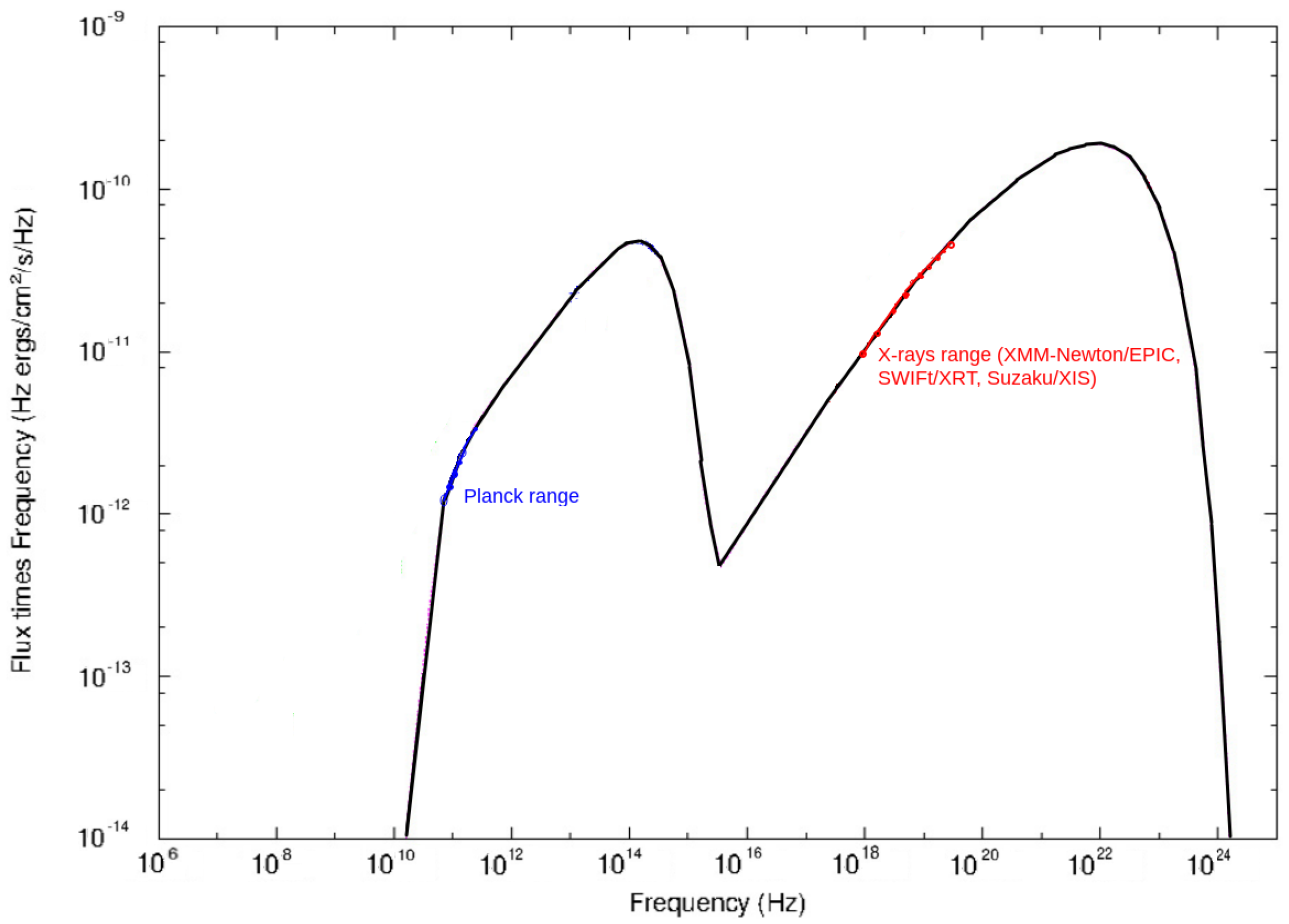
47], the jet X-ray self-Comptonized synchrotron (SSC) or Inverse Compton (IC) spectra have the same photon index as the synchrotron emission of the jet at radio wavelengths. Thus one can apply the same power-law photon index value to fit the X-ray SSC/IC and radio synchrotron emission spectra of the jet base. Taking into account that at radio frequencies the jet emission of an RL AGN is many times more intensive than the emission of other AGN components their contribution to the AGN radio spectrum is also negligible in comparison with the jet one. This makes the radio band more promising for estimation of the parameters of the synchrotron emission of the jet base. The following spectral model of 3C 111 jet emission from radio to X-rays was shown in Reference [25]; here we show their one zone SSC model with radio (Planck) and X-rays (Swift/XRT, XMM-Newton/EPIC and Suzaku/XIS) working ranges to illustrate the method we use here to determine the jet spectral counterparts (Figure 2).
In this view we propose to separate the contribution of the jet base and disk/corona based on the equality of synchrotron and SSC/IC slopes. Namely, we use for the jet base component of our X-ray spectral model the frozen values of the photon index Γ f r that is equal to that obtained from the Planck spectrum of 3C 111 in the range of 24–240 GHz. The Planck radio spectrum was fitted with a simple power-law model with the photon index Γ f r = 1.66 ± 0.06. Anyway, we here make the hypothesis about the slope and show that it allows us to reduce the tension concerning the values of the high energy cutoff.
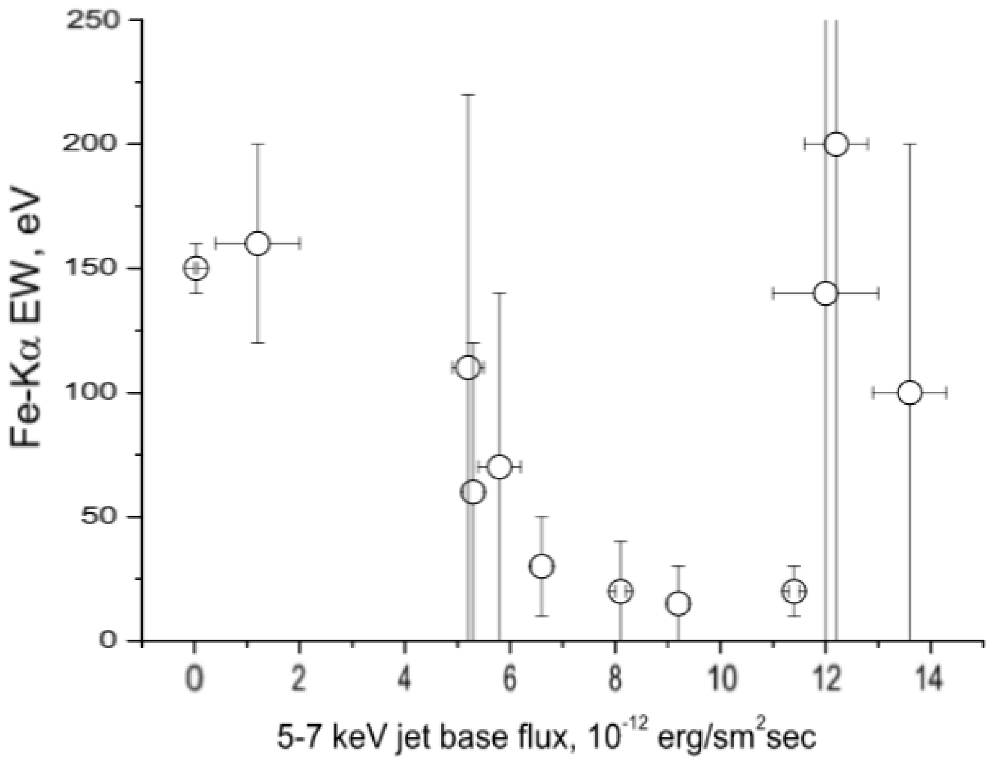
The second way we discuss here, is an use some additional information obtained from in Fe K line emission. Fe K lines emission formed in the accretion disk of an AGN is correlated with the primary nuclear continuum emitted by accretion disk/corona. Here we presume a linear dependence between Fe-K α line and primary nuclear emission fluxes.
In case of better quality data this information can serve as the basis for an alternative approach to separate the nuclear flux from the jet contributions, which presupposes that some relativistically broadened lines be present in the AGN spectrum and their equivalent width is variable.

4. Spectral Analysis

4.1. Fitting the Spectra and Separation of the Jet Base Contribution

The model of 3C 111 3.0–300 keV X-ray spectrum consists of such main components:
  • power-law continuum emission of the disk/corona F p h ( E ) = K E Γ e x p ( E / E c ) reflected or/and mildly absorbed by neutral medium, represented by pexrav model [36];
  • Fe K α line emission near 6.4 keV, represented by the Gaussian model;
  • SSC or IC emission of the jet base (the power-law with no cut-off).
We perform our fitting in the two following steps:
  • fitting the high-energy continuum excluding the 5–7 keV area where the Fe-K emission lines can be visible, with the model, including only the jet and nuclear continuum emission;
  • fitting the 5–7 keV area with the Gaussian emission line and, in the case of presence of such, absorption line also (on this step we also use the jet+nuclear continuum model with parameters frozen to the values obtained at the first step).
Keeping in mind the spin paradigm for the radio-loud AGN 3C 111, we assume that the X-ray power-law tail above 80 keV of this object is mainly due to the jet base F j e t . In this connection, we carried out the power-law fit of the total spectrum for ISGRI and BAT spectra above 80 keV to get the photon index Γ f i t ; the resulting values are shown in Table 1 (in the bottom line of each cell of the second column7). These values are mainly consistent within error limits with other calculations (except for observation period 4, where the match is marginal).
The proper and Galactic absorption N H 0 was modelled using tbabs model. The Galactic absorption was included in the model as the lowest possible value of 7.4 × 10 21 cm 2 , following Reference [37].
Additional intercalibration constants were used in the simultaneous modelling of XMM-Newton/EPIC, Suzaku/XIS or SWIFT/XRT with INTEGRAL/ISGRI or Swift/BAT spectra and its value always was in the range 0.8–1.2. The errors, lower and upper limits indicated below correspond to a 90% confidence level ( Δ χ 2 = 2.71).
Thus, in our analysis, we fitted all the components listed above with the model: p e x r a v ( Γ 0 , E c , R ) + p o ( Γ f r ) + z g a u s s ( E l i n e , σ l i n e ) ) t b a b s ( N H ) c o n s t with Γ f r =1.66.
All the spectral fits were performed using XSpec v.12.13 of HEASOFT package, version 6.27. Swift/BAT and INTEGRAL spectra were treated within the observational time intervals overlapping with shorter intervals of XMM-Newton/EPIC, Suzaku/XIS or SWIFT/XRT observations; they were processed together to trace the variability details.
Observational data are divided into 12 observational periods described in Table A5. The spectra and models are shown in the Figure A1, Figure A2, Figure A3, Figure A4, Figure A5, Figure A6, Figure A7, Figure A8, Figure A9, Figure A10, Figure A11, and Figure A12. The initial datasets involve the combined soft (XMM-Newton/EPIC, SUZAKU/XIS, or SWIFT/XRT) X-ray spectra and hard (INTEGRAL/ISGRI or SWIFT/BAT) ones collected during the same month. The intercalibration constants between these pairs of spectra are also shown.
Table 1 shows fitting parameters of the continuum spectra of 3C 111: the photon index Γ n u c l , exponential high-energy cut-off E C of the primary nuclear continuum emission, its reflection parameter R, the absorption excess N H and discrepancies χ 2 / d . o . f . of the spectral fits. Here and in Tables below, the observation periods are the same as in Table A5. The fitting has been performed with frozen value Γ f r = 1.66 of the jet base power-law SSC/IC emission. For comparison, the first column of Table 1 shows (in the bottom line) the indexes Γ f i t derived independently from the power-law fit of the high-energy tail. The results of different fittings are in satisfactory agreement within errors.
Additionally, taking into account the results of References [25,35], we performed also the fitting with the frozen value of R = R f r = 0.7 as it was shown there. As a result we can see that there are periods of higher and lower values of the reflection coefficient within the error levels (i.e., periods 1, 5–8). We can explain these variations of the reflection fraction in terms of the changes of the inner radius of the accretion disc (or its radiatively efficient zone).
Table 2 shows fitting parameters of emission spectral lines near 6 keV. In the second and third columns of this Table we show the line energy and width, and in the last one we show the equivalent widths calculated using the XSPEC12 standard procedure eqwidth. The eqwidth command calculates the equivalent width as a relation between the integrated photon flux produced by an additive model component (including in our case the line, jet and nuclear continuum), at the location of the peak of the photon spectrum (i.e., near 6.4 keV), and the flux (in units of photons per keV) at that energy of the continuum (i.e., jet + nuclear continuum in our case). The equivalent width is then defined in units of keV. The continuum (jet + nuclear) model is integrated from E Δ E to E + Δ E . The initial value of Δ E = 0.3 keV was used. Table A6 shows the absorption line parameters, which were detected during 3, 5 and 12 periods.
We also estimated the jet and primary nuclear component fluxes and the Fe-K α emission line as well basing on this model; these fluxes are shown in Table 3.

4.2. Nuclear Emission vs. Fe-K α Flux

In the previous subsection we have calculated the flux levels of the jet and primary nuclear counterparts in the spectra, basing on the spectral fitting model with the frozen value of the photon index of the jet counterpart. Here we propose another method to estimate the jet and nuclear fluxes using the results of the Fe-K α emission line fitting. The advantage of this second method is that its result depends on the emission line parameters only and not connected directly with the continuum parameters (except the flux in 5–7 keV energy range), such as photon indices of jet or primary nuclear emission. This advantage makes this method independent from the radio spectral fitting results (i.e., jet photon index).
For most measurement periods it is rather difficult to isolate Fe K α against the noise background and this is the reason of large errors of F 5 7 l i n e in Table 3 (the index 5–7 shows the energy range in keV); see also Figure 3 representing the equivalent widths of Fe K α line near 6.4 keV. Nevertheless, one can use these data in order to test some prospects for future use of F 5 7 l i n e for separation of F j e t and F n u c l provided that more accurate data be available.
In Figure 3 we arranged equivalent widths of Fe K α line vs. F 5 7 j e t in order to estimate the dependence on the jet base continuum emission levels. If we remove the unreliable data with large error bars from Figure 3, we clearly see that the larger equivalent widths correspond to lowest F 5 7 j e t . The highest value of equivalent width derived is about 150 eV (3-rd period, the left point in Figure 3 corresponding to zero jet base emission), which is compatible with the typical values of EW of RQ AGN [48]. This can be considered in favour of the similarity of the “central engine” of RQ and RL AGN. The reason leading to lower observed EW values in RL AGN than in RQ is the presence of an additional continuum component due to the jet base emission (cf. References [25,49]).
Now we consider a relation between the X-ray continuum in 5–7 keV range and flux in the Fe K α line. Reference [31] found out that the X-ray continuum flux and maximum flux in the Fe K α line are correlated with the time lag consistent with zero. For a rough estimate, we suppose that the total (energy-integrated) observed flux F 5 7 l i n e in the Fe K α line is approximately proportional to the total nucleus (disk/corona) flux in the 5–7 keV range
F 5 7 n u c l = κ F 5 7 l i n e .
Then for the total continuum flux in the 5–7 keV range we have
F 5 7 c o n t = κ F l i n e + F 5 7 j e t .
First of all, we can use the results of Section 4.1 in order to derive F 5 7 l i n e , F 5 7 j e t and κ , and then to check whether κ is the same for different observation periods. If there are periods of zero-compatible variations of the jet emission, then the alternative estimation of κ is possible. Namely, if one can assume for adjacent observation periods Δ F j e t 0, so we could derive κ from variations of the fluxes to compare with the previous results of Section 1.
In case of X-ray 3C 111 X-ray spectrum, these 5–7 keV fluxes for the three model components (power-law jet emission, primary nuclear (disk/corona) emission and Fe K α 6.4 keV emission line) are shown in Table 3. We have 3-rd period of zero-compatible jet emission with fairly good data on F 5 7 n u c l and F 5 7 l i n e , which can be used for determination of k yielding the value k = 33 ± 3. We used this value of k to estimate primary nuclear fluxes F 5 7 n u c l from values of F 5 7 l i n e using Formula (3) (Figure 4, lower panel). Despite the large errors one can see that the measured values F 5 7 n u c l fall into the interval determined the error bars of estimated F 5 7 n u c l , and the correlation coefficient between them is 0.85. This gives reason to hope that Formulas (3) and (4) can be used for independent determination of the nuclear flux in future measurements with more accurate data on the Fe K emission lines.

5. Discussion

5.1. Overview of Our Results

We had shown that there is a possibility to separate the primary nuclear and jet base contributions in the hard X-ray spectra of RL AGN 3C 111 using the observational data obtained by INTEGRAL, SWIFT and Suzaku cosmic missions during the 12 periods of observations in common even taking into account that the X-ray and radio data by Planck mission were not synchronized in time.
In order to fulfill this separation we assumed the same photon index for the X-ray component of the jet base emission and for the radio emission spectra of this object (note that the radio emission is pure jet base synchrotron and the X-ray jet base counterpart is considered as the IC or SSC emission with the same photon index as the synchrotron one).
This method shows quite accurate results and can be recommended for further usage in the other objects, but we should concede that the Planck radio spectrum is averaged upon the time and the synchrotron photon index can vary with time as well. Therefore, it would be better to have the time rows of simultaneous observations in radio- and X-rays to establish more accurate dependence between these spectra and their parameters.
We also used possible correlation between the emission levels in primary nuclear continuum and Fe K α emission lines formed in the near vicinity of the central black hole of an AGN [25,49]. The errors of the emission line parameters are quite large in most observation periods and thus give very rough estimates of the nuclear flux levels. In the same time, both approaches gave compatible results within the error bars. This gives reason to hope for the successful application of both approaches in the future for other objects, keeping in mind the necessity to have more precise spectral data for determining emission line parameters and synchronized time rows of radio- and X-ray observations.
The results of Table 1 for hard X-ray spectrum of 3C 111 show that, for the periods having modest error limits, the spectral parameters of the primary nuclear continuum (i.e., photon index and high-energy exponential cut-off) mostly do not contradict the “spin paradigm” predictions. The exception is the 6-th period, when we have the high-energy exponential cut-off of primary nuclear continuum more than ∼130 keV for the fitting with free reflection R; on the other hand the result on this period are not reliable and also we have a low E c derived with fixed R f r = 0.7 that seems to be more physical. Therefore, 3C 111 deserves further observation and analysis with better data set in the high energy region.
In the same time we have shown that the maximum value of the Fe K α line equivalent width obtained for the phase of the low level jet base emission is in agreement with the values typical for RQ AGN suggesting similarities of the “central engines” in RQ and RL AGN.

5.2. 3C 111 in γ -Rays and Further Perspectives

The emission of RL AGN above 100 keV in 3C 111 was observed at higher energies by Fermi-LAT mission [50,51,52]. The simple power-law approximation of the spectrum has been performed by Reference [50] in Fermi-LAT 10 8 –10 11 eV energy range yielding the photon index Γ = 2.7 ± 0.2. This differs significantly from the value obtained from the Planck spectrum of 3C 111; the explanation of this difference is due to different emission mechanism in γ -rays. Since then, the Fermi-LAT observational exposure of 3C 111 has increased significantly and it makes sense to analyze the extended dataset in a more detailed way in future. The higher energy ranges brings the key information about AGN jets composition as the two best known scenarios of jet formation (hadronic and leptonic) leads to the significantly different spectral shape above 10 10 –10 11 eV [53]. Leptonic scenario leads to the exponential fall of the spectrum, whereas the hadronic component produces more complicated spectral shape due to secondary pion decay. Tracing out this difference can be performed more effectively by combining the Fermi-LAT and Cherenkov Telescope Array (CTA) observational data [54].

6. Conclusions

1
We separated the “jet base” and “central engine” spectral components of AGN 3C 111 in the range from X-ray to soft γ -ray spectrum. For this purpose, we used the fixed value of the photon index from Planck radio data. We performed some tests showing that our main results are reliable. In particular, we tested the results under supposition of the linear relationship between Fe K α emission line and the 5–7 keV fluxes from the “central engine”.
2
The value of the high-energy exponential cut-off E c in the nuclear spectrum of the “central engine”, obtained after the separation of the “jet base” spectral components from the total 3C 111 spectra, are mostly below 100 keV or compatible with this within the error limits. This means that spectrum of 3C 111 “central engine” most likely does not contradict the predictions of the spin- or gap-paradigm [15,16].
3
During the phases of low jet base emission we have maximal Fe K α line equivalent widths, which are in a satisfactory agreement with the values typical for RQ AGN. This confirms the similar nature of the “central engines” of RL and RQ AGN, demonstrating that the typically lower values for most of RL AGN are due to the presence of jet base spectral counterpart, not due to physical difference in the “central engine”.

Author Contributions

Conceptualization, E.F. and A.D.P.; Data curation, B.H.; Writing—original draft, E.F. and V.Z.; Writing—review and editing, A.D.P. All authors have read and agreed to the published version of the manuscript.

Funding

This work has been supported in part by scientific program “Astronomy and space physics” (project 19BF023-01) of Taras Shevchenko National University of Kyiv.

Acknowledgments

We are grateful to the anonymous referees for useful comments, which allowed us to significantly improve the article.

Conflicts of Interest

The authors declare no conflict of interest.

Data Availability

The data treated in this article use the satellite observations with Plank, XMM-Newton, Swift, Suzaku and INREGRAL; these are described in Section 2. The data used in our work are available in HEASARC data archive (at https://heasarc.gsfc.nasa.gov/cgi-bin/W3Browse/w3browse.pl), The Neil Gehrels Swift Observatory website (https://www.swift.ac.uk/user$_$objects/docs.php) and DARTS/Suzaku (darts.isas.jaxa.jp). The datasets were derived from these three sources in the public domain (HEASARC, The Neil Gehrels Swift Observatory and DARTS/Suzaku). The observation logs are appended below in Appendix A.

Appendix A. Observational LOGs

Table A1. XMM-Newton/EPIC observations LOG. The data events from various data shown in one cell were merged together to produce one common spectrum from them.
obsIDobs. Dateobs.Time, ksecTotal EPIC Flux, ctsSNR *
006594010114-03-200144.5677515.6
055218010115-02-2009124.612,05414.5
055518020115-02-20097.8
* Signal-to-noise ratio.
Table A2. SWIFT (XRT and BAT) observations LOG.
obsIDobs. DateXRT exp., ksecXRT Flux ctsXRT ModeBAT exp. ksecBAT Flux ctsSNR
0003636700111-04-20079.64324pc9.510,9005.7
0003636700216-11-20086.32457pc6.897433.8
0003636700318-11-20081.6624pc1.4
0003636700418-01-20094.42332pc4.591015.0
0003636700509-01-20109.03476pc9.011,7903.8
0003265900128-12-20124.24578wt0.005.5
0003265900211-01-20133.86460pc/wt0.020263.2
0003265900515-01-20133.55950pc/wt0.7
0003265900620-01-20134.16970pc/wt4.1
0003265900720-01-20133.96630pc/wt0.0
0003265900808-02-20133.05400wt3.010,8106.5
0003265900910-02-20133.25440wt3.2
0003265901015-02-20133.05400wt3.0
0008196300126-12-20171.6864pc1.678814.9
Table A3. Suzaku/XIS observations LOG.
obsIDobs. Dateobs.Time, ksecTotal Flux ctsSNR
70303401022-08-2008122.420,5992.9
70504001002-09-201080.618,900
70504002009-09-201079.418,619
70504003014-09-201080.318,850
total240.356,3699.5
Table A4. INTEGRAL/ISGRI observations LOG.
Data rev.Observ. Dateobs.Time, ksecDetect. sig.
046408/200651.0
046808/20065.2
total56.27.0
064601/2008109.2
070607/200870.0
070708/200857.8
070808/200844.2
070908/200823.2
071008/200835.0
071508/200863.7
071708/200850.6
072009/200866.0
072109/200877.0
072409/2008125.8
total836.920.0
077202/200952.5
077302/200961.2
077502/2009101.2
078703/200992.5
083108/2009108.8
083208/200999.0
083308/2009128.8
083408/200944.0
083508/200968.2
083608/200959.8
total816.020.0
094807/201023.0
096008/201015.0
096108/201018.0
096208/201010.0
096309/201045.0
096509/201040.0
096609/201015.0
total166.016.0
114002/20126.3
115003/20129.5
119908/201219.0
120008/201228.5
120108/201223.4
120208/201218.5
120308/20127.6
120408/201234.2
120508/201221.0
120608/201211.0
120709/201238.0
121209/20127.6
total214.613.0
125201/201343.2
125401/201320.0
125501/20139.0
126102/201328.0
126202/20137.4
126302/20137.8
131407/201356.0
137501/20144.3
total175.89.0
150602/201530.1
151803/201531.2
156807/201544.2
157908/201544.0
158809/201536.4
186609/201713.2
191001/2018132.0
192402/2018140.0
total561.113.0
Table A5. Datasets and intercalibration constants.
N o DatesDatasetK γ
103/2001EPIC-
204/2007XRT + BAT1.5 ± 0.5
308/2008XIS + ISGRI2.0 ± 0.3
411/2008XRT + BAT + ISGRI0.5 ± 0.2
501/2009XRT + BAT + ISGRI0.9 ± 0.3
602/2009EPIC + ISGRI0.7 ± 0.2
701/2010XRT + BAT + ISGRI1.8 ± 0.5
809/2010XIS + ISGRI1.0 ± 0.1
912/2012XRT + ISGRI0.8 ± 0.1
1001/2013XRT + ISGRI0.9 ± 0.2
1102/2013XRT + BAT + ISGRI1.0 ± 0.3
1212/2017XRT + BAT + ISGRI2.02 ± 0.5
Table A6. Parameters of the absorption lines (if detected).
N o E abs , keV σ abs , keVs
35.9 ± 0.10.05 0.01 + 0.03 1.02 ± 0.03
55.9 ± 0.30.05 f r 0.22 ± 0.04
125.9 0.9 + 1.0 <0.544.2 ± 3.0

Appendix B. Spectra and Fitting Parameters

Figure A1. Unfolded XMM-Newton EPIC MOS and PN spectra of 3C 111 during 1st (March 2001) observational period and model. Above: all the spectra are shown by crosses; fitting curves are shown by solid lines; model components are shown by dotted lines; below: data residuals. During this period jet base emission was dominating slightly over nuclear one; signs of weak Fe-K α emission line are present.
Universe 06 00219 g0a1
Figure A2. Unfolded SWIFT XRT and BAT spectra of 3C 111 during 2nd observational period (April 2007) and model. Above: all the spectra are shown by crosses; fitting curves are shown by solid lines; model components are shown by dotted lines; below: data residuals. During this period jet base emission was dominating slightly over nuclear one; signs of weak Fe-K α emission line are present.
Universe 06 00219 g0a2
Figure A3. Unfolded Suzaku/XIS and INTEGRAL/ISGRI spectra of 3C 111 during 3rd observational period (August 2008) and model. Above: all the spectra are shown by crosses; fitting curves are shown by solid lines; model components are shown by dotted lines; below: data residuals. This period is remarkable as during it in the spectrum of 3C 111 was clearly visible primary nuclear component only. Fe-K α line was bright and clearly distinguishable despite the presence of absorption line near 5.9 keV.
Universe 06 00219 g0a3
Figure A4. Unfolded SWIFT/XRT, SWIFT/BAT and INTEGRAL/ISGRI spectra of 3C 111 during 4th (November 2008) observational period and model. Above: all the spectra are shown by crosses; fitting curves are shown by solid lines; model components are shown by dotted lines; below: data residuals. During this period jet base emission was dominating significantly over nuclear one (the jet base flux in 5–7 keV range was more than three times higher than the nuclear one); emission in Fe-K α line was zero-compatible.
Universe 06 00219 g0a4
Figure A5. Unfolded SWIFT/XRT, SWIFT/BAT and INTEGRAL/ISGRI spectra of 3C 111 during 5th observational period (January 2009) and model. Above: all the spectra are shown by crosses; fitting curves are shown by solid lines; model components are shown by dotted lines; below data residuals. During this period jet base and nuclear emission components were on the same level; signs of Fe-K α emission line and absorption line near 5.9 keV are present.
Universe 06 00219 g0a5
Figure A6. Unfolded XMM-Newton/EPIC (MOS and PN) and INTEGRAL/ISGRI spectra of 3C 111 during 6th observational period and model. Above: all the spectra are shown by crosses; fitting curves are shown by solid lines; model components are shown by dotted lines; below: data residuals. During this period bot primary nuclear continuum and jet base emission were visible; jet component is quasi two times brighter in 5–7 keV energy range. Weak Fe-K α line was visible, but no signs of absorption features near 5.9 keV.
Universe 06 00219 g0a6
Figure A7. Unfolded SWIFT/XRT and INTEGRAL/ISGRI spectra of 3C 111 during 7th (January 2010) observational period and model. Above: all the spectra are shown by crosses; fitting curves are shown by solid lines; model components are shown by dotted lines; below: data residuals. During this period nuclear emission was dominating significantly over jet base one; despite the quite poor quality of the XRT spectrum the signs of weak Fe-K α emission line are visible.
Universe 06 00219 g0a7
Figure A8. Unfolded Suzaku/XIS and INTEGRAL/ISGRI spectra of 3C 111 during 8th observational period (September 2010) and model. Above: all the spectra are shown by crosses; fitting curves are shown by solid lines; model components are shown by dotted lines; below: data residuals. During this period nuclear emission was zero-compatible, as well as the Fe-K α emission line. This spectrum can be considered as a pure jet base emission.
Universe 06 00219 g0a8
Figure A9. Unfolded Swift/XRT and SWIFT/BAT spectra of 3C 111 during 9th observational period (December 2012) and model. Above: all the spectra are shown by crosses; fitting curves are shown by solid lines; model components are shown by dotted lines; below: data residuals. During this period jet base emission was dominating significantly over nuclear one (the jet base flux in 5–7 keV range was more than three times higher than the nuclear one); emission in Fe-K α line was zero-compatible.
Universe 06 00219 g0a9
Figure A10. Unfolded SWIFT/XRT, SWIFT/BAT and INTEGRAL/ISGRI spectra of 3C 111 during 10th (January 2013) observational period and model. Above: all the spectra are shown by crosses; fitting curves are shown by solid lines; model components are shown by dotted lines; below: data residuals. During this period jet base emission was dominating significantly over nuclear one (the jet base flux in 5–7 keV range was near six times higher than the nuclear one); emission in Fe-K α line was zero-compatible.
Universe 06 00219 g0a10
Figure A11. Unfolded SWIFT/XRT and INTEGRAL/ISGRI spectra of 3C 111 during 11th observational period (February 2013) and model. Above: all the spectra are shown by crosses; fitting curves are shown by solid lines; model components are shown by dotted lines; below: data residuals. During this period jet base and nuclear emission components were on the same level; Fe-K α emission line is clearly present.
Universe 06 00219 g0a11
Figure A12. Unfolded SWIFT/XRT and SWIFT/BAT spectra of 3C 111 during 12th (December 2017) observational period and model. Above: all the spectra are shown by crosses; fitting curves are shown by solid lines; model components are shown by dotted lines; below: data residuals. During this period jet base emission was dominating over nuclear one (the jet base flux in 5–7 keV range was near as twice as higher than the nuclear one); emission in Fe-K α line was weak; also the tiny signs of the weak absorption line near 5.9 were present.
Universe 06 00219 g0a12

References

  1. Kellermann, K.I.; Sramek, R.; Schmidt, M.; Shaffer, D.B.; Green, R. VLA observations of objects in the Palomar Bright Quasar Survey. Astron. J. 1989, 98, 1195–1207. [Google Scholar] [CrossRef]
  2. Marecki, A.; Swoboda, B. The transition from quasar radio-loud to radio-quiet state in the framework of the black hole scalability hypothesis. Astron. Astrophys. 2011, 525, A6. [Google Scholar] [CrossRef]
  3. Fender, R.P.; Belloni, T.M.; Gallo, E. Towards a unified model for black hole X-ray binary jets. Mon. Not. R. Astron. Soc. 2004, 355, 1105–1118. [Google Scholar] [CrossRef] [Green Version]
  4. Fender, R.P.; Homan, J.; Belloni, T.M. Jets from black hole X-ray binaries: Testing, refining and extending empirical models for the coupling to X-rays. Mon. Not. R. Astron. Soc. 2009, 396, 1370–1382. [Google Scholar] [CrossRef] [Green Version]
  5. Motta, S. Quasi-periodic oscillations in black-hole binaries. In The Extremes of Black Hole Accretion; Ness, J.U., Ed.; European Space Astronomy Centre: Madrid, Spain, 2016; p. 10. [Google Scholar]
  6. Lohfink, A.M.; Reynolds, C.S.; Jorstad, S.G.; Marscher, A.P.; Miller, E.D.; Aller, H.; Aller, M.F.; Brenneman, L.W.; Fabian, A.C.; Miller, J.M.; et al. An X-Ray View of the Jet Cycle in the Radio-loud AGN 3C120. Astrophys. J. 2013, 772, 83. [Google Scholar] [CrossRef]
  7. Padovani, P.; Urry, C.M. Fanaroff-Riley I galaxies as the parent population of BL Lacertae objects. I—X-ray constraints. Astrophys. J. 1990, 356, 75–82. [Google Scholar] [CrossRef]
  8. Sambruna, R.M.; Tombesi, F.; Reeves, J.N.; Braito, V.; Ballo, L.; Gliozzi, M.; Reynolds, C.S. The Suzaku view of 3C 382. Astrophys. J. 2011, 734, 105. [Google Scholar] [CrossRef]
  9. Sulentic, J.W.; Zwitter, T.; Marziani, P.; Dultzin-Hacyan, D. Eigenvector 1: An Optimal Correlation Space for Active Galactic Nuclei. Astrophys. J. 2000, 536, 5–9. [Google Scholar] [CrossRef] [Green Version]
  10. Capetti, A.; Balmaverde, B. The host galaxy/AGN connection in nearby early-type galaxies: A new view of the origin of the radio-quiet/radio-loud dichotomy? Astron. Astrophys. 2006, 453, 27–37. [Google Scholar] [CrossRef]
  11. Kozieł-Wierzbowska, D.; Vale Asari, N.; Stasińska, G.; Sikora, M.; Goettems, E.I.; Wójtowicz, A. What Distinguishes the Host Galaxies of Radio-loud and Radio-quiet AGNs? Astrophys. J. 2017, 846, 42. [Google Scholar] [CrossRef] [Green Version]
  12. Wilson, A.S.; Colbert, E.J.M. The difference between radio-loud and radio-quiet active galaxies. Astrophys. J. 1995, 438, 62–71. [Google Scholar] [CrossRef] [Green Version]
  13. Meier, D.L. The Association of Jet Production with Geometrically Thick Accretion Flows and Black Hole Rotation. Astrophys. J. 2001, 548, L9–L12. [Google Scholar] [CrossRef] [Green Version]
  14. Blandford, R.D.; Znajek, R.L. Electromagnetic extraction of energy from Kerr black holes. Mon. Not. R. Astron. Soc. 1977, 179, 433–456. [Google Scholar] [CrossRef]
  15. Garofalo, D. Signatures of black hole spin in the cosmological evolution of galaxies. In American Astronomical Society Meeting Abstracts #214; Bulletin of the American Astronomical Society: Washington, DC, USA, 2009; Volume 41, p. 684. [Google Scholar]
  16. Garofalo, D. Retrograde versus Prograde Models of Accreting Black Holes. Adv. Astron. 2013, 2013, 213105. [Google Scholar] [CrossRef] [Green Version]
  17. Reynolds, C.S. Measuring Black Hole Spin Using X-Ray Reflection Spectroscopy. Space Sci. Rev. 2014, 183, 277–294. [Google Scholar] [CrossRef] [Green Version]
  18. Rusinek, K.; Sikora, M.; Kozieł-Wierzbowska, D.; Gupta, M. On the diversity of the jet production efficiency in Swift/BAT AGNs. arXiv 2020, arXiv:2006.11049. [Google Scholar] [CrossRef]
  19. Blandford, R.D.; Payne, D.G. Hydromagnetic flows from accretion disks and the production of radio jets. Mon. Not. R. Astron. Soc. 1982, 199, 883–903. [Google Scholar] [CrossRef] [Green Version]
  20. Meyer, F.; Liu, B.F.; Meyer-Hofmeister, E. Black hole X-ray binaries: A new view on soft-hard spectral transitions. Astron. Astrophys. 2000, 354, L67–L70. [Google Scholar]
  21. Meyer, F.; Liu, B.F.; Meyer-Hofmeister, E. Evaporation: The change from accretion via a thin disk to a coronal flow. Astron. Astrophys. 2000, 361, 175–188. [Google Scholar]
  22. Narayan, R. Low-Luminosity Accretion in Black Hole X-Ray Binaries and Active Galactic Nuclei. Astrophys. Space Sci. 2005, 300, 177–188. [Google Scholar] [CrossRef]
  23. Körding, E.G.; Jester, S.; Fender, R. Accretion states and radio loudness in active galactic nuclei: Analogies with X-ray binaries. Mon. Not. R. Astron. Soc. 2006, 372, 1366–1378. [Google Scholar] [CrossRef] [Green Version]
  24. Fedorova, E.; Vasylenko, A.; Zhdanov, V. Peculiar AGNs from the INTEGRAL and RXTE data. Bull. Taras Shevchenko Natl. Univ. Kyiv Astron. 2017, 55, 29–34. [Google Scholar] [CrossRef] [Green Version]
  25. De Jong, S.; Beckmann, V.; Mattana, F. The nature of the multi-wavelength emission of 3C 111. Astron. Astrophys. 2012, 545, A90. [Google Scholar] [CrossRef] [Green Version]
  26. King, A.L.; Lohfink, A.; Kara, E. AGN Coronae through a Jet Perspective. Astrophys. J. 2017, 835, 226. [Google Scholar] [CrossRef] [Green Version]
  27. Tortosa, A.; Bianchi, S.; Marinucci, A.; Matt, G.; Petrucci, P.O. A NuSTAR census of coronal parameters in Seyfert galaxies. Astron. Astrophys. 2018, 614, A37. [Google Scholar] [CrossRef] [Green Version]
  28. Gupta, M.; Sikora, M.; Rusinek, K.; Madejski, G.M. Comparison of hard X-ray spectra of luminous radio galaxies and their radio-quiet counterparts. Mon. Not. R. Astron. Soc. 2018, 480, 2861–2871. [Google Scholar] [CrossRef] [Green Version]
  29. Sguera, V.; Bassani, L.; Malizia, A.; Dean, A.J.; Landi, R.; Stephen, J.B. Is 3C 111, an apparently normal radio galaxy, the counterpart of 3EG J0416+3650? Astron. Astrophys. 2005, 430, 107–113. [Google Scholar] [CrossRef]
  30. Sargent, W.L. Redshifts for six 3CR radio galaxies and the spectrum of 3C 111. Astrophys. J. 1977, 212, 105–106. [Google Scholar] [CrossRef]
  31. Chatterjee, R.; Marscher, A.P.; Jorstad, S.G.; Markowitz, A.; Rivers, E.; Rothschild, R.E.; McHardy, I.M.; Aller, M.F.; Aller, H.D.; Lähteenmäki, A.; et al. Connection Between the Accretion Disk and Jet in the Radio Galaxy 3C 111. Astrophys. J. 2011, 734, 43. [Google Scholar] [CrossRef] [Green Version]
  32. Reynolds, C.S.; Iwasawa, K.; Crawford, C.S.; Fabian, A.C. X-ray spectroscopy of the broad-line radio galaxy 3C 111. Mon. Not. R. Astron. Soc. 1998, 299, 410–416. [Google Scholar] [CrossRef] [Green Version]
  33. Ballo, L.; Braito, V.; Reeves, J.N.; Sambruna, R.M.; Tombesi, F. The high-energy view of the broad-line radio galaxy 3C 111. Mon. Not. R. Astron. Soc. 2011, 418, 2367–2380. [Google Scholar] [CrossRef] [Green Version]
  34. Tombesi, F.; Sambruna, R.M.; Reeves, J.N.; Reynolds, C.S.; Braito, V. X-ray evidence for the accretion disc-outflow connection in 3C 111. Mon. Not. R. Astron. Soc. 2011, 418, L89–L93. [Google Scholar] [CrossRef] [Green Version]
  35. Beckmann, V.; De Jong, S.; Mattana, F.; Saez, D.; Soldi, S. Gamma-ray emitting radio galaxies at hard X-rays: Seyfert core or jet emission? In Proceedings of the “An INTEGRAL View of the High-Energy Sky (The First 10 Years)”—9th INTEGRAL Workshop and Celebration of the 10th Anniversary of the Launch (INTEGRAL 2012), Paris, France, 15–19 October 2012; p. 58. [Google Scholar]
  36. Magdziarz, P.; Zdziarski, A. Angle-dependent Compton reflection of X-rays and gamma-rays. Mon. Not. R. Astron. Soc. 1995, 273, 837–848. [Google Scholar] [CrossRef] [Green Version]
  37. Tombesi, F.; Reynolds, C.S.; Mushotzky, R.F.; Behar, E. Excess Galactic molecular absorption toward the radio galaxy 3C 111. Astrophys. J. 2017, 842, 64–69. [Google Scholar] [CrossRef] [Green Version]
  38. Kalberla, P.M.W.; Burton, W.B.; Hartmann, D.; Arnal, E.M.; Bajaja, E.; Morras, R.; Pöppel, W.G.L. The Leiden/Argentine/Bonn (LAB) Survey of Galactic HI. Final data release of the combined LDS and IAR surveys with improved stray-radiation corrections. Astron. Astrophys. 2005, 440, 775–782. [Google Scholar] [CrossRef]
  39. Grossberger, C.; Kadler, M.; Wilms, J.; Müller, C.; Beuchert, T.; Ros, E.; Ojha, R.; Aller, M.; Aller, H.; Angelakis, E.; et al. Structural Variability of 3C111 on Parsec Scales. Acta Polytech. 2012, 52, 18. [Google Scholar]
  40. Schulz, R.; Kadler, M.; Ros, E.; Krichbaum, T.P.; Grossberger, C.; Mueller, C.; Mannheim, K.; Agudo, I.; Aller, H.D.; Aller, M.F. mm-VLBI observations of the active galaxy 3C111 in outburst. In Proceedings of Science; Vol.178—The 11th European VLBI Network Symposium & Users Meeting, Bordeaux, France, 9–12 October 2012; PoS-sissa: Trieste, Italy, 2016. [Google Scholar] [CrossRef] [Green Version]
  41. Clautice, D.; Perlman, E.S.; Georganopoulos, M.; Lister, M.L.; Tombesi, F.; Cara, M.; Marshall, H.L.; Hogan, B.; Kazanas, D. The Spectacular Radio-near-IR-X-Ray Jet of 3C 111: The X-Ray Emission Mechanism and Jet Kinematics. Astrophys. J. 2016, 826, 109. [Google Scholar] [CrossRef]
  42. Beuchert, T.; Kadler, M.; Perucho, M.; Großberger, C.; Schulz, R.; Agudo, I. VLBA polarimetric monitoring of 3C 111. Astron. Astrophys. 2018, 610, A32. [Google Scholar] [CrossRef] [Green Version]
  43. Schulz, R.; Kadler, M.; Ros, E.; Perucho, M.; Krichbaum, T.P.; Agudo, I.; Beuchert, T.; Lindqvist, M.; Mannheim, K.; Wilms, J.; et al. Sub-milliarcsecond imaging of a bright flare and ejection event in the extragalactic jet 3C 111. arXiv 2020, arXiv:2009.01294. [Google Scholar] [CrossRef]
  44. La Mura, G.; Busetto, G.; Ciroi, S.; Rafanelli, P.; Berton, M.; Congiu, E.; Cracco, V.; Frezzato, M. Relativistic plasmas in AGN jets. From synchrotron radiation to γ-ray emission. Eur. Phys. J. D 2017, 71, 95. [Google Scholar] [CrossRef] [Green Version]
  45. Beckmann, V.; Shrader, C.R. Active Galactic Nuclei; Wiley-VCH Verlag GmbH: Hoboken, NJ, USA, 2012; 350p, ISBN 978-3527410781. [Google Scholar]
  46. Wilson, A.S. X-ray emission processes in extragalactic jets, lobes and hot spots. New Astron. Rev. 2003, 47, 417–421. [Google Scholar] [CrossRef] [Green Version]
  47. Condon, J.J.; Ransom, S.M. Essential Radio Astronomy; Princeton University Press: Princeton, NJ, USA, 2016; ISBN 978-0-691-13779-7. [Google Scholar]
  48. Gofford, J.; Reeves, J.N.; Tombesi, F.; Braito, V.; Turner, T.J.; Miller, L.; Cappi, M. The Suzaku view of highly ionized outflows in AGN – I. Statistical detection and global absorber properties. Mon. Not. R. Astron. Soc. 2013, 430, 60–80. [Google Scholar] [CrossRef] [Green Version]
  49. Fukazawa, Y.; Finke, J.; Stawarz, Ł.; Tanaka, Y.; Itoh, R.; Tokuda, S. Suzaku Observations of γ-Ray Bright Radio Galaxies: Origin of the X-Ray Emission and Broadband Modeling. Astrophys. J. 2015, 798, 74. [Google Scholar] [CrossRef] [Green Version]
  50. Kataoka, J.; Stawarz, Ł.; Takahashi, Y.; Cheung, C.C.; Hayashida, M.; Grandi, P.; Burnett, T.H.; Celotti, A.; Fegan, S.J.; Fortin, P.; et al. Broad-line Radio Galaxies Observed with Fermi-LAT: The Origin of the GeV γ-Ray Emission. Astrophys. J. 2011, 740, 29. [Google Scholar] [CrossRef] [Green Version]
  51. Grandi, P.; Torresi, E.; Stanghellini, C. The γ-Ray Emission Region in the Fanaroff-Riley II Radio Galaxy 3C 111. Astrophys. J. 2012, 751, L3. [Google Scholar] [CrossRef] [Green Version]
  52. Sahakyan, N.; Baghmanyan, V.; Zargaryan, D. Fermi-LAT observation of nonblazar AGNs. Astron. Astrophys. 2018, 614, A6. [Google Scholar] [CrossRef] [Green Version]
  53. Boettcher, M.; Reimer, A.; Sweeney, K.; Prakash, A. Leptonic and Hadronic Modeling of Fermi-Detected Blazar. Astrophys. J. 2013, 768, 54–68. [Google Scholar] [CrossRef] [Green Version]
  54. Acharya, B.S.; Agudo, I.; Al Samarai, I.; Alfaro, R.; Alfaro, J.; Alispach, C.; Alves Batista, R.; Amans, J.P.; Amato, E.; Ambrosi, G.; et al. Science with the Cherenkov Telescope Array; World Scientic Publishing Co. Pte. Ltd.: Singapore, 2019. [Google Scholar] [CrossRef] [Green Version]
1
2
3
4
5
6
7
For the first period we have not obtained a reliable value.
Figure 1. Observational periods of XMM-Newton, Suzaku and SWIFT missions.
Universe 06 00219 g001
Figure 2. The radio-to-X-rays multiwavelength spectral energy distribution of 3C 111 within the one-zone SSC model [25], shown by black solid line. The frequency range of Planck is shown by blue zone and X-rays range corresponding to Swift/XRT, XMM-Newton/EPIC and Suzaku/XIS is shown by red.
Universe 06 00219 g002
Figure 3. Fe K α line EW vs. F 5 7 j e t * .
Universe 06 00219 g003
Figure 4. Fluxes in Fe K α line and primary nuclear ones for 12 observational periods derived by different methods. Upper panel: measured fluxes F 5 7 l i n e * in Fe K α line. Lower panel: Primary nuclear flux within 5–7 keV energy range F 5 7 n u c l * , estimated using dependence (3) between nuclear and Fe K α line emission (yellow circles with error bars, “prediction”) and F 5 7 n u c l * of Table 3 (blue balls, “fitted model”).
Universe 06 00219 g004
Table 1. Hard X-ray continuum parameters with marginal errors (90% probability) for 3C 111. First lines in each cell include nuclear continuum parameters estimated with the frozen value of the jet base emission index Γ f r :index Γ n u c l , exponential cutoff energy E c and reflection coefficient R of the nuclear emission. The second lines present analogous fit with frozen Γ f r and frozen reflection coefficient R f r = 0.7 as it was obtained by Reference de Jong et al. [25]. The lower lines of the first column show the jet emission indexes Γ f i t (free) from the independent power-law fit of the spectral tail for E > 80 keV. First column: observational period; second to fifths columns: photon index, high-energy cut-off and reflection of primary nuclear emission; fifth column: absorbing column density excess in comparison with the Galactic absorption; sixth column: chi-squared/degrees-of-freedom.
N o Γ nucl E c , keVRN H * χ 2 / d . o . f .
11.7 ± 0.4-<7.00.5 ±   0.1 2162.0/2022
1.7 ± 0.2-0.7 f r 0.5 ± 0.1 2162.4/2023
21.2 1.0 + 1.5 98 73 + <13.00.5 ± 0.5122.3/120
1.3 1.0 + 1.3 100 80 + 0.7 f r 0.5 ± 0.5122.4/121
1.7 ± 0.5
31.84 0.04 + 0.28 250 120 + 0.9 ±   0.5 0.5 ± 0.3598.7/559
1.83 0.06 + 0.26 745 650 + 0.7 f r 0.5 ± 0.3599.4/560
1.3 ± 0.5
40.6 0.1 + 0.2 35 10 + 22 <13.00.11 0.08 + 0.09 115.2/104
0.84 ±   0.3 58 ±   40 0.7 f r 0.11 0.08 + 0.09 118.3/105
1.7 ± 0.7
51.5 ± 0.1181 66 + 285 0.8 ± 0.7<1.133.1/33
1.5 ± 0.9183 113 + 353 0.7 f r <1.136.0/34
1.2 ± 0.7
61.48 ± 0.02>1330.5 ± 0.3<1.02359.5/1966
1.45 ± 0.09175 175 + 255 0.7 f r <1.02361.2/1967
1.7 ± 0.5
71.53 ± 0.0739 15 + 23 <0.253.0 ± 1.568.6/52
1.3 ± 0.48 2 + 4 0.7 f r 3.0 ± 1.572.5/53
1.84 ± 0.41
81.68 ± 0.03132 42 + 80 0.15 ± 0.07<0.32130.2/2220
1.3 ± 0.211 2 + 4 0.7 f r <0.32228.0/2221
1.8 ± 0.9
91.7 ± 0.330 10 + <1.5<2.169.1/60
1.7 ± 0.440 25 + 0.7 f r <2.169.1/61
1.50 ± 0.9
101.6 ± 0.318 10 + 380 7<60.8 ± 0.1144.8/114
1.4 0.3 + 0.4 15 ± 70.7 f r 0.8 ± 0.1145.9/115
1.5 ± 0.7
112.3 0.5 + 0.4 24 14 + 50 <5.51.9 ± 1.497.8/95
2.0 0.2 + 0.4 13 5 + 20 0.7 f r 1.9 ± 1.498.8/96
1.5 ±   0.7
121.70 ± 0.1530 19 + 21 <7.01.4 ± 0.516.1/13
1.2 0.3 + 0.6 13 ± 50.7 f r 1.4 ± 0.516.7/14
1.3 0.5 + 0.6
* 10 22 cm 2 .
Table 2. Fe K α line emission parameters. First column: observational period; second column: line energy; third column: line width; fourth column: equivalent width.
N o E line , keV σ line , keVEW, keV
16.4 f r 0.17 0.17 + 0.12 0.02 0.01 + 0.02
26.4 f r 0.08 0.08 + 0.02 0.06 ± 0.06
36.39 ± 0.030.07 ± 0.020.15 ± 0.01
46.4 f r < 7 × 10 5 <0.03
56.4 f r 0.05 ± 0.050.11 0.11 + 0.24
66.38 ± 0.030.05 ± 0.030.03 ± 0.02
76.25 ± 0.120.2 0.2 + 0.4 0.16 ± 0.04
86.4 f r 0.04 ± 0.020.02 ± 0.01
96.4 f r 0.05 ± 0.050.1 ± 0.1
106.33 ± 0.090.02 0.02 + 0.50 0.14 ± 0.14
116.4 f r 0.2 ± 0.20.2 0.2 + 0.5
126.4 f r 0.01 ± 0.010.07 ± 0.07
Table 3. 5–7 keV fluxes for various model components. First column: observational period; second column: jet flux in 5–7 keV energy range; third column: nuclear flux in 5–7 keV energy range; fourth column: Fe-K α emission line flux in 5–7 keV energy range.
N o F 5 7 jet * F 5 7 nucl * F 5 7 line *
18.1 ± 0.16.5 ± 0.10.2 ± 0.1
25.3 ± 0.24.4 ± 0.20.2 ± 0.2
30.03 ± 0.033.61 ± 0.010.11 ± 0.01
49.2 ± 0.22.2 ± 0.20.1 0.1 + 0.2
55.2 ± 0.35.6 ± 0.30.3 ± 0.3
66.6 ± 0.23.6 ± 0.20.2 ± 0.1
71.2 0.8 + 0.4 11.3 0.1 + 0.8 0.4 ± 0.1
811.4 ± 0.10.1 ± 0.10.1 ± 0.1
913.6 ± 0.71.2 ± 0.70.1 ± 0.1
1012 ± 12.2 ± 1.00.9 ± 0.9
1112.2 ± 0.69.0 ± 0.60.2 0.2 + 0.6
125.8 ± 0.42.8 ± 0.40.001 0.001 + 0.4
* 10 12 erg/cm 2 · /sec.
Publisher’s Note: MDPI stays neutral with regard to jurisdictional claims in published maps and institutional affiliations.

