Review

Gravity with Higher Derivatives in D-Dimensions

by
Sergey G. Rubin
1,2,
Arkadiy Popov
2,* and
Polina M. Petriakova
1
1
Moscow Engineering Physics Institute, National Research Nuclear University MEPhI, Kashirskoe shosse 31, 115409 Moscow, Russia
2
N.I. Lobachevsky Institute of Mathematics and Mechanics, Kazan Federal University, Kremlevskaya Street 18, 420008 Kazan, Russia
*
Author to whom correspondence should be addressed.
Universe 2020, 6(10), 187; https://doi.org/10.3390/universe6100187
Submission received: 25 September 2020 / Revised: 12 October 2020 / Accepted: 13 October 2020 / Published: 20 October 2020

Abstract

:
The aim of this review is to discuss the ways to obtain results based on gravity with higher derivatives in D-dimensional world. We considered the following ways: (1) reduction to scalar tensor gravity, (2) direct solution of the equations of motion, (3) derivation of approximate equations in the presence of a small parameter in the system, and (4) the method of test functions. Some applications are presented to illustrate each method. The unification of two necessary elements of a future theory is also kept in mind—the extra dimensions and the extended form of the gravity.

1. Introduction

Higher derivative theories of gravity is widely used in modern research despite the internal problems inherent in this approach [1,2]. One such problem is the Ostrogradsky instabilities [3]. The f ( R ) -gravity is the simplest extension of the Einstein–Hilbert theory of gravity, which is free from Ostrogradsky instabilities. Reviews of f ( R ) —theories, including extension to the Gauss–Bonnet gravity, can be found in [4,5]. The specific form of the function f ( R ) was considered in [6,7,8].
Another widespread idea, the world with extra dimensions is considered as the necessary element for a complete fundamental theory. The idea of extra dimensions is also used to explain cosmological evolution [9]. The invisibility of extra dimensions can be explained by their small size smaller than 10 18 cm.
One of the aims of our research is to combine two main elements of future theory—the gravity with higher derivatives and the extra dimensions. The latter could reveal itself at the inflationary energies and higher.
It is generally assumed that our Universe was born at Planck energies and evolved by expanding and cooling to its present state. The inflationary stage is characterized by sub-Planckian energy density and looks inevitable. A description of the spontaneous creation of the Universe with the inflationary regime can be found in [10]. Models describing the inflation have been elaborated using many different ingredients, like supersymmetry [11] and attracting the inflationary idea for explanation of another cosmological problems like primordial black holes [12,13], dark matter [14], and baryogenesis [15]. For review, see, for example, [16,17] and references therein. Since the energy scale at the inflationary stage of the evolution of the Universe is high enough, some quantum effects may be manifested and responsible for the inflationary regime. Two typical elements of quantum gravity can play a role in the construction of inflationary models: nonlinear geometrical extensions of Einstein’s theory of gravity and extra dimensions. Moreover, the quantization of gravity requires a nonlinear geometric extension of the Einstein–Hilbert action. The first formulation of the inflationary model, the Starobinsky model [18], considers nonlinear geometric terms belonging to the class of f ( R ) theories.
To our knowledge, there are four ways to move forward in the framework of higher derivative theories of gravity in D-dimensions:
  • Reduction of action to the scalar tensor gravity. This way is effective for the action in the form
    S = m D D 2 2 d D Z | g D | f ( R ) .
  • Direct solution to equations of motion.
  • Derivation of approximate equations provided that a system contains a small parameter.
  • Method of trial functions.
The next sections are devoted to their discussion.
Throughout this paper, we use the following conventions: R A B C D = C Γ A B D B Γ A C D + Γ E C D Γ B A E Γ E B D Γ A C E , R M N = R M F N F .

2. Reduction of Action to the Scalar-Tensor Gravity

f ( R ) theories of gravity or, more generally, higher derivative theories of gravity are now widely used as a tool for theoretical research. The interest in f ( R ) theories is motivated by inflationary scenarios of the evolution of the Universe, starting with Starobinsky’s pioneering work [18]. A number of viable f ( R ) models in four-dimensional space-time satisfying the observable constraints are discussed in [19,20,21].
The first method is based mostly on the conformal transformations that lead to the standard form of Einstein’s gravitational action. The price is the appearance of the additional dynamic variable in the form of the scalar field. Necessary formulas for the D-dim space are represented in the section below.

2.1. Conformal Transformations in D Dimensions

Action (1) can be reduced to a scalar-tensor model in two steps. Firstly, consider the action depending on auxiliary scalar field χ
S S T = m D D 2 2 d D Z | g D | [ f ( χ ) R + f ( χ ) f ( χ ) χ ]
One of the classical equation is
f ( χ ) ( R χ ) = 0
Thus, χ = R provided that f ( χ ) 0 . Substituting this into (2), we arrive to initial action (1). These actions are equivalent at the classical level.
As the second step is based on the well known conformal transformation, see e.g., [22]
g A B = | Ω | 2 D 2 g ^ A B ,
which leads to the Ricci scalar transformation in the form
g D Ω R = ( s i g n Ω ) g ^ D R ^ + D 1 D 2 A Ω g ^ A B B Ω Ω 2 + d i v .
Here, all letters with hat are functions of g A B ^ , and d i v denotes a full divergence which does not contribute to the field equations.
Application of the conformal transformation (4) with Ω = f to expression (2) gives
S = 1 2 d D x | g ^ D | [ R ^ + ( ψ ) 2 2 V ( ψ ) ]
where
ψ = D 2 D 1 ln f ( χ )
( m D = 1 ) and
V ( ψ ) = e D ( D 1 ) ( D 2 ) ψ U ( χ ) , U ( χ ) 1 2 ( f ( χ ) χ f ( χ ) ) .
The Lagrangian containing the Ricci scalar in the form of specific function f ( R ) is transformed into the scalar-tensor model that strongly simplifies the subsequent calculations. The applications are wide and can be found in a set of publications [4,19,20,21,23]. Here, we consider one of the applications concerning the Starobinsky model of inflation [18].

2.2. The Starobinsky Model

This model provides the best fit to the observational data at present times. Historically, this was the first model of inflation, but many models containing the scalar field(s) were intensively discussed during a couple of decades. These models are well elaborated and intuitively clear.
The model in question is described by the action (1) with D = 4 and f ( R ) = R + R 2 / 6 M 2 . As one can see from the previous section, the conformal transformation leads to the scalar-tensor model of inflation, allowing the application of already known results [24]. Indeed, action (2) is the starting point for the inflationary models based on a scalar field dynamic. According to (8), the potential has the form
V ( ψ ) = 3 4 m 4 2 M 2 1 e 2 / 3 ψ / m 4 2
We have obtained an effective model containing the Einstein–Hilbert action and the scalar field in the standard form. The scalar field potential possesses a profound minimum at ψ = 0 . The later is a necessary element responsible for the field oscillations and hence the reheating just after the end of inflation. The ground state energy should also be zero with great accuracy due to the extreme smallness of the cosmological constant.
A variety of inflationary models that differ in the form of the potential are described by action (6). Most of them are based on the slow motion of fields and should satisfy some conditions which characterized the inflationary stage. The slow roll parameters are defined as
ϵ = 1 2 ( V V ) 2 ,
η = V V ,
ξ 2 = V V V 2 .
The main parameters are the scalar/tensorial relative amplitude r and the scalar spectral index n s , besides the running of the spectral index d n s / d ln k , which are given, in terms of the slow roll parameters, as
n s = 1 6 ϵ + 2 η ,
r = 16 ϵ ,
d n s d ln k = 16 ϵ η + 24 ϵ 2 + 2 ξ 2 .
k is the wavenumber.
According to [16], the observed values are as follows:
n s 0.968 , r < 0.1 , d n s d ln k = 0.0045 ± 0.0067 .
The potential (9) satisfies all of them for M 10 5 . Notice that this potential has only one parameter, M, and nevertheless gives the best fit to the observations.
We see that the method of conformal transformations allows us to apply the well-known results elaborated for the scalar fields, thus making the physical picture clearer. The known flaws of this approach are (a) quantum correspondence before and after the conformal transformations is suspicious, (b) treating more general forms of Lagrangian is not easy.
Let us discuss the second way—numerical solution to the proper system of equations.

3. Direct Solution to Equations of Motion

We will illustrate this way for two cases:
  • f ( R ) gravity,
  • f ( R ) + Gauss–Bonnet gravity.

3.1. f ( R ) Gravity

Let a D = 1 + d 1 + d 2 -dimensional space-time T × M d 1 × M d 2 appeared as a result of some quantum processes at high energies. The probability of these processes is a subtle point, and we do not discuss it in this article. It is supposed that manifolds are born with a random shape. The entropy growth in T × M d 1 × M d 2 manifold leads to the entropy minimization of subspace M d 2 [25]. We begin our research after completing symmetrization and investigate the classical evolution of subspaces M d 1 and M d 2 whose metric
d s 2 = d t 2 e 2 β 1 ( t ) d Ω 1 2 e 2 β 2 ( t ) d Ω 2 2
is assumed to be maximally symmetrical with a positive curvature. In this section, we consider the action in the form (1). The equations of this theory are known,
1 2 f ( R ) δ A B + R A B + A B δ A B f R = 0 .
The nontrivial equations of system (18) are
1 2 f ( R ) + f R e 2 β 1 ( t ) ( d 1 1 ) + β ¨ 1 + β ˙ 1 ( d 1 β ˙ 1 + d 2 β ˙ 2 ) + ( 1 d 1 ) β ˙ 1 d 2 β ˙ 2 f R R R ˙ f R R R R ˙ 2 f R R R ¨ = 0 ,
1 2 f ( R ) + f R e 2 β 2 ( t ) ( d 2 1 ) + β ¨ 2 + β ˙ 2 ( d 1 β ˙ 1 + d 2 β ˙ 2 ) + ( 1 d 2 ) β ˙ 2 d 1 β ˙ 1 f R R R ˙ f R R R R ˙ 2 f R R R ¨ = 0 ,
1 2 f ( R ) + d 1 β ¨ 1 + d 2 β ¨ 2 + d 1 β ˙ 1 2 + d 2 β ˙ 2 2 f R d 1 β ˙ 1 + d 2 β ˙ 2 f R R R ˙ = 0
in terms of metric (17). Here, we took into account that t f R = f R R R ˙ and t 2 f R = f R R R R ˙ 2 + f R R R ¨ . The Ricci scalar is
R = d 1 β ¨ 1 + d 2 β ¨ 2 + d 1 β ˙ 1 2 + d 2 β ˙ 2 2 + d 1 e 2 β 1 ( t ) ( d 1 1 ) + β ¨ 1 + β ˙ 1 ( d 1 β ˙ 1 + d 2 β ˙ 2 ) + d 2 e 2 β 2 ( t ) ( d 2 1 ) + β ¨ 2 + β ˙ 2 ( d 1 β ˙ 1 + d 2 β ˙ 2 ) .
The system of Equations (19)–(21) is a system of fourth-order differential equations with respect to unknown functions β 1 ( t ) and β 2 ( t ) . Note that this system is not solvable with respect to the highest derivatives β 1 and β 2 because these derivatives appear when expression (22) is substituted into the similar terms f R R R ¨ of Equations (19) and (20). Therefore, two equations contain the forth-order derivatives with equal multipliers.
Another way to solve the problem is as follows: we can consider R ( t ) as an additional unknown function, and the expression (22) as the fourth equation of the system. In this case, we obtain a system of second order ordinary differential equations for the unknown functions β 1 ( t ) , β 2 ( t ) , and R ( t ) . Three equations of this system (for example, (19), (20), (22)) can be solved with respect to β ¨ 1 , β ¨ 2 , R ¨ . Then, substitution β ¨ 2 and β ¨ 1 into Equation (21) gives equation
10 d 1 β ˙ 1 + d 2 β ˙ 2 f R R R ˙ + 5 R 5 d 1 ( d 1 1 ) β ˙ 1 2 10 d 1 d 2 β ˙ 1 β ˙ 2 5 d 2 ( d 2 1 ) β ˙ 2 2 5 d 1 ( d 1 1 ) e 2 β 1 5 d 2 ( d 2 1 ) e 2 β 2 f R 5 f ( R ) = 0 ,
which plays the role of restriction for our system of differential equations. Equation (23) should be used to obtain a relation between the initial data β 1 ( t 0 ) , β ˙ 1 ( t 0 ) , β 2 ( t 0 ) , β ˙ 2 ( t 0 ) , and R ˙ ( t 0 ) . The value R ( 0 ) can be found from auxiliary condition (23) at t = 0 . Let
f ( R ) = a 3 R 3 + a 2 R 2 + a 1 R + a 0
with the parameter values (the choice is quite arbitrary)
a 0 = 0.6 , a 1 = 1 , a 2 = 2 , a 3 = 1.3 .
Figure 1 shows the numerical solution of the system of Equations (19), (20), and (22) in different time ranges. The region of small values of time is shown at the left panel. The time behavior of both functions β 1 ( t ) and β 2 ( t ) differ from each other due to differences in the initial conditions, see the capture of Figure 1. The panel in the middle indicates similar asymptotic behavior of the solutions. The more detailed figure on the right panel helps distinguish the functions β 1 ( t ) and β 2 ( t ) .
The asymptotics of the solution
β 1 ( t ) = H 1 t , β 2 ( t ) = H 2 t ( H 1 > 0 , H 2 > 0 ) .
are determined by the Equations (19)–(22) at t
R ( t ) = d 1 ( d 1 + 1 ) H 1 2 + d 2 ( d 2 + 1 ) H 2 2 + 2 d 1 d 2 H 1 H 2 R 0 ,
f R d 1 H 1 2 + d 2 H 1 H 2 1 2 f R = R 0 = 0 ,
f R d 2 H 2 2 + d 1 H 1 H 2 1 2 f R = R 0 = 0 ,
f R d 1 H 1 2 + d 2 H 2 2 1 2 f R = R 0 = 0 .
According to these equations, the subspaces are expanded with equal speed,
H 1 = H 2 = f 2 ( d 1 + d 2 ) f R R = R 0 .
Using this expression, we obtain the equation for R 0 from (27)
( d 1 + d 2 + 1 ) f R = R 0 + 2 R f R R = R 0 = 0 .
We note that the results at t do not depend on the initial conditions and H 1 , H 2 , R 0 are consistent with the numerical results. Nevertheless, the conclusion that the asymptotic behavior is independent of the initial conditions in their whole range is hasty. As shown in Figure 2, for some initial conditions, there is no stable solution.
The discussion above indicates that time dependence of an extra space metric is determined by the initial conditions. The latter leads to growing volumes of both extra spaces, which means that such solutions are hardly applicable to the description of our Universe.
In a more realistic situation, the radius of one of the subspaces (say, M d 2 ) remains constant
β 2 ( t ) = β c = c o n s t ,
while the other one, M d 1 , expands. In this case, the system of Equations (19)–(22) admits an analytic solution. More definitely, the combination d 1 · (19) d 1 · (20) + (21) f R · (22) gives
f ( R ) 2 + R ( t ) + d 1 + d 2 d 2 ( d 1 + d 2 ) e β c f R = 0 .
It means that
R ( t ) = R 0 = c o n s t
and R 0 can be found from Equation (33). Then, Equations (19)–(22) can be rewritten as
R 0 = 2 d 1 β ¨ 1 + d 1 ( d 1 + 1 ) β ˙ 1 2 + d 1 ( d 1 1 ) e 2 β 1 ( t ) + d 2 ( d 2 1 ) e 2 β c ,
1 2 f ( R 0 ) + f R e 2 β 1 ( t ) ( d 1 1 ) + β ¨ 1 + d 1 β ˙ 1 2 R = R 0 = 0 ,
1 2 f ( R 0 ) + e 2 β c ( d 2 1 ) f R R = R 0 = 0 ,
1 2 f ( R 0 ) + d 1 β ¨ 1 + β ˙ 1 2 f R R = R 0 = 0 .
Subtracting Equation (36) from (38), we obtain
( d 1 1 ) β ¨ 1 e 2 β 1 ( t ) f R R = R 0 = 0 ,
which gives the connection
β ¨ 1 = e 2 β 1 ( t )
for d 1 1 , f R R = R 0 0 . Then, Equations (35)–(38) are reduced to
e 2 β 1 ( t ) + β ˙ 1 2 = e 2 β c ( d 2 1 ) d 1 = f ( R ) 2 d 1 f R R = R 0 = R 0 d 2 ( d 2 1 ) e 2 β c d 1 ( d 1 + 1 ) H 2 .
The solution of Equations (41) and (40) with respect to β 1 ( t ) is
β 1 ( t ) = ± H t t 0 + ln 1 + e 2 H ( t t 0 ) 2 H , H > 0 ,
where H , R 0 and β c can be found from the last relations (41).
In this section, we have obtained a set of numerical and analytical solutions in f ( R ) gravity. Dependence on the initial conditions appears to be nontrivial. The relation between the initial conditions and the asymptotes of the solutions is also not clear.

3.2. Starobinsky Model, Direct Calculation

Let us come back to Starobinsky model discussed above and perform the direct simulations. Both approaches should give similar results. To this end, consider the four-dimensional theory described by the action
S [ g μ ν ] = 1 2 m P l 2 d 4 x | g 4 | f ( R ) .
The corresponding equations of motion in four dimensions are as follows:
f R ( R ) R μ ν 1 2 f ( R ) g μ ν + μ ν g μ ν f R ( R ) = 0 , g μ ν μ ν
with μ , ν = 1 , 2 , 3 , 4 . Taking into account the choice of the metric of the three-dimensional sphere
d s 2 = g μ ν d x μ d x ν = d t 2 e 2 α ( t ) d x 2 + sin 2 x d y 2 + sin 2 x sin 2 y d z 2
we obtain the system of equations
6 α ˙ ( t ) R ˙ ( t ) f R ( R ) 6 α ¨ ( t ) + α ˙ 2 ( t ) f R ( R ) + f ( R ) = 0 , 2 R ˙ 2 ( t ) f R ( R ) + 2 R ¨ ( t ) + 2 α ˙ ( t ) R ˙ ( t ) f R ( R ) 2 α ¨ ( t ) + 6 α ˙ 2 ( t ) + 4 e 2 α ( t ) f R ( R ) + f ( R ) = 0 ,
where the definition of the Ricci scalar for metric (45) is
R ( t ) = 12 α ˙ 2 ( t ) + 6 α ¨ ( t ) + 6 e 2 α ( t ) .
Let us choose the form of the function as in the Starobinsky model
f ( R ) = R 2 6 M 2 + R ,
where M is a constant parameter with dimension of mass and is defined as
M 1.5 · 10 5 m P l 50 N e , N e = 55 ÷ 60 .
Using the second equation of the system (46) and the definition of the Ricci scalar (47), we get
R ¨ ( t ) = 2 α ˙ ( t ) R ˙ ( t ) 1 12 R 2 ( t ) + α ˙ 2 ( t ) + e 2 α ( t ) M 2 R ( t ) + 3 M 2 α ˙ 2 ( t ) + e 2 α ( t ) , α ¨ ( t ) = 2 α ˙ 2 ( t ) e 2 α ( t ) + 1 6 R ( t ) .
The second derivative α ¨ ( t ) is disappeared in a combination of the first equation of the system (46) and definition of the Ricci scalar (47). Finally, we obtain the quadratic equation
R 2 ( t ) 12 α ˙ 2 ( t ) + e 2 α ( t ) R ( t ) 12 α ˙ ( t ) R ˙ ( t ) 36 M 2 α ˙ 2 ( t ) + e 2 α ( t ) = 0 .
This expression being substituted into the first equation of the system (50), leads to the equation of free damped harmonic oscillations
R ¨ ( t ) + 3 α ˙ ( t ) R ˙ ( t ) + M 2 R ( t ) = 0 .
We need to choose the initial conditions to find a solution for the unknown functions α ( t ) and R ( t ) . Let the initial conditions on the function α ( t ) in Planck units be given as
α ( 0 ) α 0 = ln H i n f l = ln 10 6 13.8 , α ˙ ( 0 ) α 1 = H i n f l 10 6 .
Solving the previously obtained Equation (51), we find an expression for the function R ( t ) at the initial time depending on the value of other initial conditions
R ( 0 ) R 0 = 6 α 1 2 + e 2 α 0 ± 36 α 1 2 + e 2 α 0 2 + 12 α 1 R 1 + 36 M 2 α 1 2 + e 2 α 0 .
Thus, after substitution of specific values of quantities, we get
R ˙ ( 0 ) R 1 = 0 ( 54 ) R + ( 0 ) = 2.9 · 10 11 , R ( 0 ) = 4.3 · 10 12 .
The result of numerical solving the system (50) with the choice of the initial conditions (53) and (55) is presented in Figure 3. The time interval of inflation is between 10 42 s and 10 36 s and is equal on the Planck scale to ∼20 and ∼2 · 10 7 , respectively. The slope of the straight line for the function α ( t ) changes at a value of time close to the end of inflation, where oscillations of the curvature R ( t ) begin. This is shown on the right side of Figure 3. The origin of these oscillations is clear from the Equation (52). When a regime 1.5 α ˙ ( t ) < M occurs in this equation, the solution is damped oscillations. This condition leads to the spacetime being considered flat or of small curvature: at the inflation stage, R 12 H I n f l 2 = 12 α ˙ 2 ( t ) | R | < < M 2 10 10 . The size of the space at the inflation stage should increase by 10 26 times and, for the function α ( t ) , it is a value of about 60; we see that the result shown in Figure 3 confirms this fact. Numerical calculation gives the value of the Hubble constant in Planck units H I n f l α ˙ ( t ) 10 6 within the required order during inflation.
Asymptotic behavior can be found after reconstruction of the numerical solution. The size of the sphere exp { α ( t U n i v ) } exp { 154 } , the curvature value R ( t U n i v ) 10 122 and the value of the derivative of the function α ˙ ( t U n i v ) 10 61 .
As a result, the direct numerical simulation and application of the conformal transformation give similar results and may be used if a Lagrangian is not very complicated.

3.3. f ( R ) + Gauss–Bonnet Gravity

In this section, we extend our study to action in the more complex form
S e f f = 1 2 m D D 2 d D x | g D | f ( R ) + c 1 R A B R A B + c 2 R A B C D R A B C D .
This action represents an example of the effective theory [26]. Here, c 1 , c 2 are parameters of the Lagrangian, and f ( R ) is a function of the Ricci scalar R. The Gauss–Bonnet Lagrangian
L G B = k g { R 2 4 R A B R A B + R A B C D R A B C D }
belongs to such set of models and is the appropriate starting point because of the absence of higher derivatives.
The action
S g e n = 1 2 m D D 2 d D x | g D | [ f ˜ ( R ) + k { R 2 4 R A B R A B + R A B C D R A B C D } ]
is used in the following. This action is the particular case of the action (56) provided that f ˜ ( R ) = f ( R ) k R 2 and c 1 = 4 k , c 2 = k . In what follows, we will consider only the quadratic function
f ( R ) = a R 2 + b R + c
( b = 1 without the loss of generality).
We assume that both subspaces are three-dimensional maximally symmetric subspaces of positive curvature
d s 2 = d t 2 e 2 α ( t ) m D 2 [ d x 2 + sin 2 ( x ) d y 2 + sin 2 ( x ) sin 2 ( y ) d z 2 ] e 2 β ( t ) m D 2 [ d θ 2 + sin 2 ( θ ) d ϕ 2 + sin 2 ( θ ) sin 2 ( ϕ ) d ψ 2 ] .
Einstein’s equations for this model are
1 2 f ˜ ( R ) δ B A + ( R B A + A B δ B A ) f ˜ R + k [ 8 R A C ; B C 12 R A C R C B + 2 δ B A R C D R C D δ B A 2 R C D E F R C D E F + 2 R A C D E R B C D E + 4 R ; A ; B + 4 R C A D B · R C D δ B A 2 R 2 + 2 R R B A ] = 0 ,
The nontrivial system of Equation (61) is
36 k α ˙ β ˙ 3 + 3 α ˙ 2 β ˙ 2 + α ˙ 3 β ˙ + e 2 α β ˙ β ˙ + α ˙ + e 2 β α ˙ β ˙ + α ˙ + e 2 β e 2 α 3 f ˜ R R R ˙ α ˙ + β ˙ + 3 f ˜ R α ¨ + β ¨ + α ˙ 2 + β ˙ 2 1 2 f ˜ ( R ) = 0 ,
12 k 2 α ¨ β ˙ α ˙ + β ˙ + β ¨ α ˙ 2 + 4 α ˙ β ˙ + β ˙ 2 + 2 α ˙ 3 β ˙ + 6 α ˙ 2 β ˙ 2 + 6 α ˙ β ˙ 3 + β ˙ 4 + e 2 α β ¨ + 2 β ˙ 2 + e 2 β 2 α ¨ + β ¨ + 3 α ˙ 2 + 2 α ˙ β ˙ + β ˙ 2 + e 2 α e 2 β f ˜ R R R R ˙ 2 f ˜ R R R ¨ + R ˙ 2 α ˙ + 3 β ˙ + f ˜ R α ¨ + 3 α ˙ 2 + 3 α ˙ β ˙ + 2 e 2 α 1 2 f ˜ ( R ) = 0 ,
12 k α ¨ α ˙ 2 + 4 α ˙ β ˙ + β ˙ 2 + 2 β ¨ α ˙ α ˙ + β ˙ + α ˙ 4 + 6 α ˙ 3 β ˙ + 6 α ˙ 2 β ˙ 2 + 2 α ˙ β ˙ 3 + e 2 α α ¨ + 2 β ¨ + α ˙ 2 + 2 α ˙ β ˙ + 3 β ˙ 2 + e 2 β α ¨ + 2 α ˙ 2 + e 2 α e 2 β f ˜ R R R R ˙ 2 f ˜ R R R ¨ + R ˙ 3 α ˙ + 2 β ˙ + f ˜ R β ¨ + 3 α ˙ β ˙ + 3 β ˙ 2 + 2 e 2 β 1 2 f ˜ ( R ) = 0 ,
where we have kept in mind denotations t ( f ˜ R ) = f ˜ R R R ˙ and t 2 ( f ˜ R ) = f ˜ R R R R ˙ 2 + f ˜ R R R ¨ . The Ricci scalar is
R = 6 β ¨ + α ¨ + 2 β ˙ 2 + 3 α ˙ β ˙ + 2 α ˙ 2 + e 2 β + e 2 α .
Here, and in the following, the units m D = 1 are assumed.
As in Section 3.1, it is convenient to consider the Ricci scalar R ( t ) as the additional unknown function and interpret definition (65) as the fourth equation of the system with respect to unknown functions α ( t ) , β ( t ) , and R ( t ) . Three equations of this system (for example, (63)–(65)) can be solved with respect to the higher derivatives α ¨ , β ¨ , R ¨ . Then, substituting α ¨ and β ¨ into Equation (62), we obtain the equation
36 k α ˙ 3 β ˙ + 3 α ˙ 2 β ˙ 2 + α ˙ β ˙ 3 + e 2 α β ˙ α ˙ + β ˙ + e 2 β α ˙ α ˙ + β ˙ + e 2 α e 2 β 3 α ˙ + β ˙ R ˙ f ˜ R R + 3 α ˙ 2 9 α ˙ β ˙ 3 β ˙ 3 e 2 α 3 e 2 β + R 2 f ˜ R f ˜ 2 = 0 ,
The standard initial conditions are not independent due to Equation (66). The latter must be used to obtain a relation between these initial data.
The free parameters a k m D 2 , c m D 2 are not related to the observational values because of the strong and uncontrolled contribution of the quantum corrections at sub-Planckian energies.
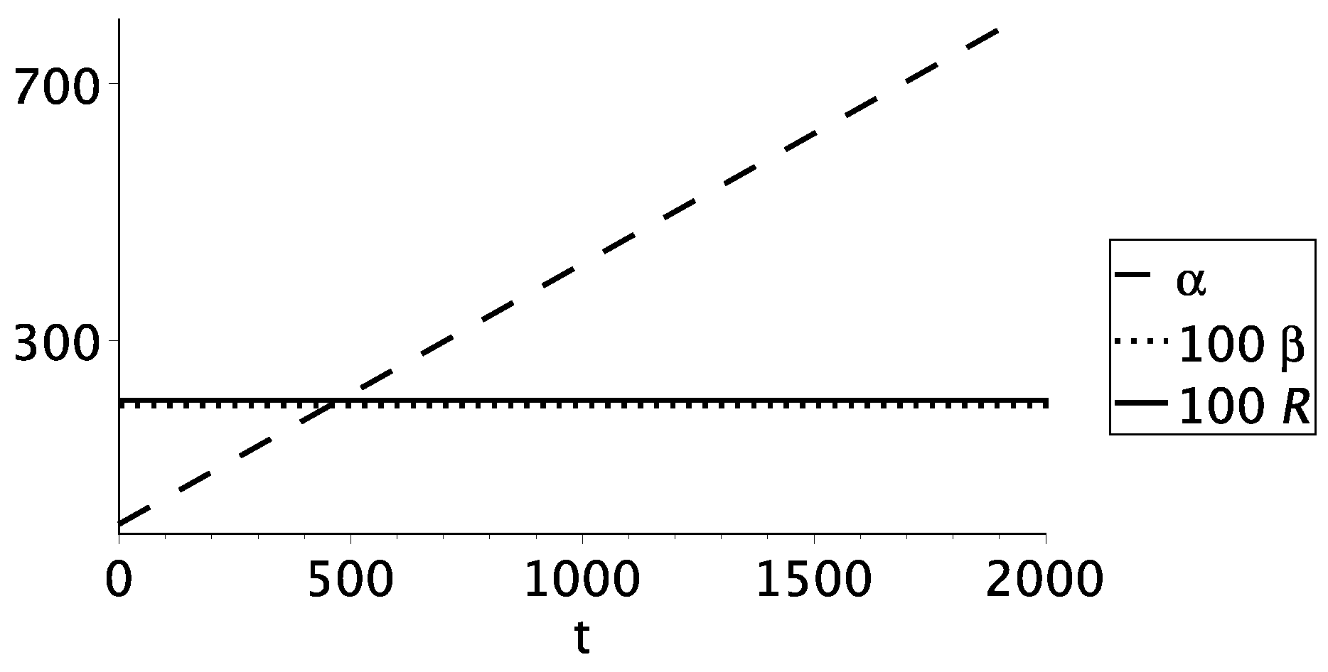
An example of numerical solution to system (62)–(64) is represented in Figure 4.
The choice of another set of physical parameters can change the picture. Sub-spaces grow at different rates as is represented in Figure 5 and Figure 6.

4. Approximate Method

The gravity with higher derivatives provides us with new abilities in understanding the role of metric in the observed world. The price is that the analysis becomes much more complicated. The attraction of extra dimensions aggravates the situation. Fortunately, a small parameter arises naturally, provided that the extra space is small and compact. Let us accept for estimation that the average Ricci scalar R n of the extra space relates to its size r n as R n 1 / r n 2 . This means that R n is in many orders of magnitude larger than the 4-dim Ricci scalar.
As a result, small parameter
ϵ R 4 / R n 1
appears that strongly facilitate an analysis. Below, we follow the method developed in [27]

4.1. Basic Idea

Consider the gravity with higher derivatives (1). The metric is assumed to be the direct product M 4 × V n of the 4-dim space M 4 and n-dim compact space V n
d s 2 = g 6 , A B d z A d z B = g 4 , μ ν ( x ) d x μ d x μ + g n , a b ( y ) d y a d y b .
Here, g 4 , μ ν is a metric of the manifolds M 4 and g n , a b ( y ) is a metric of the manifolds V n . x and y are the coordinates of the subspaces M 4 and V n , respectively. We will refer to 4-dim space M 4 and n-dim compact space V n as the main space-time and an extra space, respectively. The metric has the signature (+ - - - ...), the Greek indexes μ , ν = 0 , 1 , 2 , 3 refer to 4-dimensional coordinates. Latin indexes run over a , b = 4 , 5 , . . . .
According to (68), the Ricci scalar represents a simple sum of the Ricci scalar of the main space and the Ricci scalar of extra space
R = R 4 + R n .
In this section, the extra space is assumed to be maximally symmetric so that its Ricci scalar R n = c o n s t .
Using inequality (67) the Taylor expansion of f ( R ) in Equatiom (1) gives
S = m D D 2 2 d 4 x d n y | g 4 ( x ) | | g n ( y ) | f ( R 4 + R n ) m D D 2 2 d 4 x d n y | g 4 ( x ) | | g n ( y ) | [ R 4 ( x ) f ( R n ) + f ( R n ) ]
The prime denotes derivation of functions on its argument. Thus, f ( R ) stands for d f / d R in the formula written above. Comparison of the second line in expression (70) with the Einstein–Hilbert action
S E H = M P 2 2 d 4 x | g ( x ) | ( R 2 Λ )
gives the expression
M P 2 = m D D 2 v n f ( R n )
for the Planck mass. Here, v n is the volume of the extra space. The term
Λ m D D 2 2 M P l 2 v n f ( R n )
represents the cosmological Λ term. Both the Planck mass and the Λ term depend on a function f ( R ) . Notice that, according to (72), the Planck mass could be smaller than D-dim Planck mass, M P l < m D for specific functions f that could lead to nontrivial consequences.

4.2. Extension of the Model: Low Energies

The quantum fluctuations of metric produce all possible terms that are invariant under the coordinate transformations [26,28]. We extend our study to effective action in the form (56)
S g e n = 1 2 m D D 2 d D x g D [ f ( R ) + c 1 R A B R A B + c 2 R A B C D R A B C D ] .
Another point is that the extra space metric depends on all coordinates, not only those describing extra dimensions. Therefore, the small parameter method should be expanded for this more general case.
In this section, we use small parameter (67) and the conformal transformations analogous to conformal transformations (4) to clarify the classical behavior of system acting in D dimensions.
Here, we consider a D = 4 + n - dimensional manifold M , having the simplest geometric structure of a direct product, M = M 4 × M n , with the metric
d s 2 = d t 2 e α ( x ) d r 2 + r 2 ( d θ 2 + sin 2 ( θ ) d φ 2 e 2 β ( x ) d Ω n 2 .
It is assumed that the extra space is n-dimensional maximally symmetrical manifold with positive curvature.
The size of extra dimensions is supposed to be small compared to the size of our 4-dim space so that inequality (67) holds and we may follow the method elaborated in [27,29]. According to (75), the Ricci scalar is
R = R 4 + R n + P k ; P k = + n ( n + 1 ) ( β ) 2 + 2 n β + 6 n μ α μ β .
The additional inequality
P k R n
means that fluctuations of the 4-dim metric coefficient β ( x ) are smooth. More specifically,
| μ g A B | ϵ | a g A B | , ϵ 1 .
Using Formulas (68)–(77), we can perform the Taylor decomposition of the function f ( R ) to transform the action as
S = 1 2 v n d d 0 x g 0 e d 2 β n [ f ( R n ) R 4 + f ( R n ) P k + f ( R n ) +
+ c 1 R A B R A B + c 2 R A B C D R A B C D ] ,
R n = ϕ = n ( n 1 ) e 2 β ( x ) , R A B R A B = ( n 1 ) 2 n e 4 β + 2 n ( n 1 ) e 2 β ( β 2 + n ( β ) 2 + 4 μ α μ β ) + O ( ϵ 4 ) , R A B C D R A B C D = 2 n 1 n e 4 β + 4 n ( n 1 ) e 2 β ( β ) 2 + O ( ϵ 4 ) .
The action of the form (79) is written in the Jordan frame. We consider this frame as a ”physical” one which gives us the Planck mass, in particular
M P 2 = v n f ( ϕ m ) ; v n = 2 π n + 1 2 Γ ( n + 1 2 ) e n β m .
Here, ϕ m delivers a minimum of V E ( ϕ ) (see definition (85) below).
It is more familiar to work in the Einstein frame. To this end, we have to perform the conformal transformation (4)
g a b g a b ( E ) = e n β | f ( ϕ ) | g a b , ϕ R n = n ( n 1 ) e 2 β ( x )
of the metric describing the subspace M 4 . This leads to the action in the Einstein frame in form
S l o w = 1 2 v n d 4 x g 4 s i g n ( f ) [ R 4 + K ( ϕ ) ( ϕ ) 2 2 V ( ϕ ) ] ,
K ( ϕ ) = 1 4 ϕ 2 6 ϕ 2 ( f / f ) 2 2 n ϕ ( f / f ) + 1 2 n ( n + 2 ) + c 1 + c 2 f ϕ ,
V ( ϕ ) = s i g n ( f ) 2 f 2 | ϕ | n ( n 1 ) n / 2 f ( ϕ ) + c V n ϕ 2 , c V = c 1 + 2 c 2 ( n 1 )
representing specific Lagrangian of the scalar-tensor gravity [27]. Here, D = 4 + n and the physical meaning of the effective scalar field ϕ is the Ricci scalar of the extra space.
An important remark is necessary. The action (79) describes the field evolution at high energies in the Jordan frame. When the scalar field is settled in its minimum, we should express the 4-dim Planck mass according to (81). Simultaneously, the scalar field is evolving during inflation, and it is worth using the Einstein frame to facilitate analysis. In this case, we should consider
m 4 v n
as the effective Planck mass during the inflation in the Einstein frame.
Let us impose restrictions that follow from the observational data at low energies. In this case, observable value of the cosmological constant is extremely small and we neglect it. We also assume that the field ϕ is in its stationary state. Thus, necessary conditions are as follows:
V ( ϕ m ) = 0 ; V ( ϕ m ) = 0 .
The inequalities
ϕ m > 0 , f ( ϕ m ) > 0 , K ( ϕ m ) > 0 . V ( ϕ m ) = m 2 > 0
are necessary to consider the field ϕ as the scalar field with the standard properties. The function f ( R ) should be specified to make specific predictions. It is chosen in the form
f ( R ) = a R 2 + b R + c .
One can easily solve algebraic Equation (87) with respect to
ϕ m = b 2 ( a + c V / n )
and
c = b 2 4 ( a + c V / n ) .
Our 4-dimensional space-time is surely not Minkowskian so that the relation (91) holds approximately.
Let’s consider inequalities (88) in more detail. The first inequality in (88) leads to
b 2 a + c V / n > 0 .
The second inequality in (88) gives
f ( ϕ m ) > 0 b c V / n a + c V / n > 0 . or c V < 0
The third inequality in (88) gives the inequality
12 a 2 + 4 a c V + c V 2 n + 2 c V 2 4 c V ( c 1 + c 2 ) > 0 ,
and the fourth equality in (88) leads to
V ( ϕ m ) = b n 2 c V 2 a + c V / n b 3 b 2 ( a + c V / n ) n ( n 1 ) n / 2 m 2 > 0 i . e . b > 0 .
As the result, the parameters of action must satisfy the conditions
b > 0 , c V < 0 , a + c V / n < 0 .
The presence of a small parameter permits solving two problems. The consideration is reduced to the standard Einstein gravity + scalar field, and four dimensions appear naturally because the integration of the extra coordinate is trivial. The potential of the scalar field is promising from the point of view appropriate inflationary scenario. We show below how to elaborate the inflationary model.

4.3. Extension of the Model: Moderate Energies

The study above indicates that some limits on the Lagrangian parameter values can be derived in this approach’s framework. Nevertheless, freedom in the choice of the parameter values remains. This freedom that is used below can be used to obtain e.g., appropriate inflationary models, see [30,31] for details.
First of all, we have to specify our action (83) by definition of the function f ( R ) (89). The final form of the action is
S = m 4 2 2 d 4 x g 4 sign ( 2 a ϕ + b ) { R + K ( ϕ ) ϕ ; ρ ϕ ; ρ 2 V ( ϕ ) } ,
where
m 4 = V n = 2 π n + 1 2 Γ ( n + 1 2 ) , m D = 1 ,
and
K ( ϕ ) = 1 ϕ 2 ( 2 a ϕ + b ) 2 { [ ( 6 n + n 2 2 ) a 2 + 2 ( c 1 + c 2 ) a ] ϕ 2
+ [ n 2 2 a b + ( c 1 + c 2 ) b ] ϕ + n ( n + 2 ) 8 b 2 } ,
V ( ϕ ) = sign ( 2 a ϕ + b ) 2 ( 2 a ϕ + b ) 2 [ ϕ n ( n 1 ) n / 2 ( a + c V n ) ϕ 2 + b ϕ + c } ,
and
c V = c 1 + 2 c 2 n 1 .
The kinetic factor K ( ϕ ) and the potential K ( ϕ ) have a complex form depending on several parameters. They are represented in Figure 7 for the parameter values
n = 2 , b = 1 , a = 2 , c V = 8 , c K = 15000 , c V = c 1 + 2 c 2 n 1 , c K = c 1 + c 2 .
The parameter c can be obtained from expression (91). Restrictions (88)–(95) are also taken into account.
Finally, we must check inequality (67) (written in the Jordan frame) to be sure in the self-consistency of our approach. The n-dim scalar Ricci is not transformed under conformal transformations (82) so that R 2 = ϕ . Let us estimate the 4-dim part of the Ricci scalar R 4 keeping in mind the slow motion regime which is inherent for the inflationary period. In this case, R 4 ( E ) = 12 H 2 12 · 8 π V ( ϕ ) / 3 M P l 2 in the Einstein frame. A relation to the Jordan frame may be found in (4), (5), and (82). Finally,
ϵ R 4 ( J ) / R n 100 f ( ϕ ) V ( ϕ ) / ϕ 2 .
Our approximation (67) holds if the field ϕ is varied near the potential minimum, ϕ = ϕ m , in the region where the potential is limited from above
V ( ϕ ) ϕ m 2 100 f ( ϕ m ) 10 4
Here, ϕ m = 0.083 in the units m D = 1 according to the figure above. As we will see just below, m D 0.1 M P l so that the limitation (104) is not very restricted: V 10 8 M P l 4 .
In the main text above, we express all quantities in units m D = 1 with the effective Planck mass m 4 defined by (86). Finally, when the scalar field ϕ has been settled in the minimum of its potential V ( ϕ ) , one should restore more physical units valid for the Jordan frame, i.e., the Planck units using the relation (81). For chosen parameter values (102), the relation
M P l = V n e n β m f ( ϕ m ) m D
can be used to obtain the value of the D-dimensional Planck mass. For two-dimensional extra space ( n = 2 , V 2 = 4 π ),
M P l = V 2 e 2 β m f ( ϕ m ) m D = 8 π ( 2 a + 1 ϕ m ) m D 10 m D ,
which means that the D-dim Planck mass m D is in the order of magnitude smaller than the Planck mass in the Jordan frame.
One can see that the presence of a small parameter strongly facilitates the analysis and could lead to promising results, even if the initial system is quite complicated. Indeed, it is hard even to guess that action (74) could adequately describe the inflationary stage. On the other side, the energy density at the moderate energies (inflation) is not small, so that one must check the smallness of the parameter value (67).

5. Method of Trial Functions

This method is applied if a system in question is too complicated, see, e.g., [32,33]. The mathematically correct way to deal with gravitational systems is as follows. One should type equations of motion for a metric of the most general form, and solves it for desired initial and boundary conditions. The freedom in the coordinate choice facilitates the analysis, but the system often remains too complicated to be solved. The problem is usually solved by choosing a limited set of metrics that is substituted into an action. Classical equations are obtained by variation of the metric belonging to the chosen set. The well-known example is the minisuperspace model of Universe creation. The method of trial functions is one of such a sort. Its essence is to choose an appropriate set of metrics—some functions depending on parameters. The action appears to be dependent on the set of unknown parameters. The classical system of equations is reduced to an algebraic system for these parameters.
Let us illustrate it by the specific solution that non trivially connects two sub-spaces. Consider a manifold M with topology T × M 1 × M 2 × M 3 , where M 1 is one-dimensional, infinite space, and M 2 , M 3 are two-dimensional spheres. We study the pure gravitational field action in the form (74) with the metric
d s 2 = A ( u ) d t 2 A ( u ) 1 d u 2 e 2 β 1 ( u ) d Ω 1 2 e 2 β 2 ( u ) d Ω 2 2 .
Here, A ( u ) , β 1 ( u ) , and β 2 ( u ) are members of the limited set of metrics depending on the Schwarzschild radial coordinate u, < u < . The action contains invariants depending on these functions. For example, the Ricci scalar has the form (see [34,35] for details)
R = 2 e 2 β 1 + 2 e 2 β 2 A 4 A β 1 + β 2
2 A 3 β 1 2 + 3 β 2 2 + 4 β 1 β 2 + 2 β 1 + 2 β 2 ,
with prime denoting differentiation with respect to u.
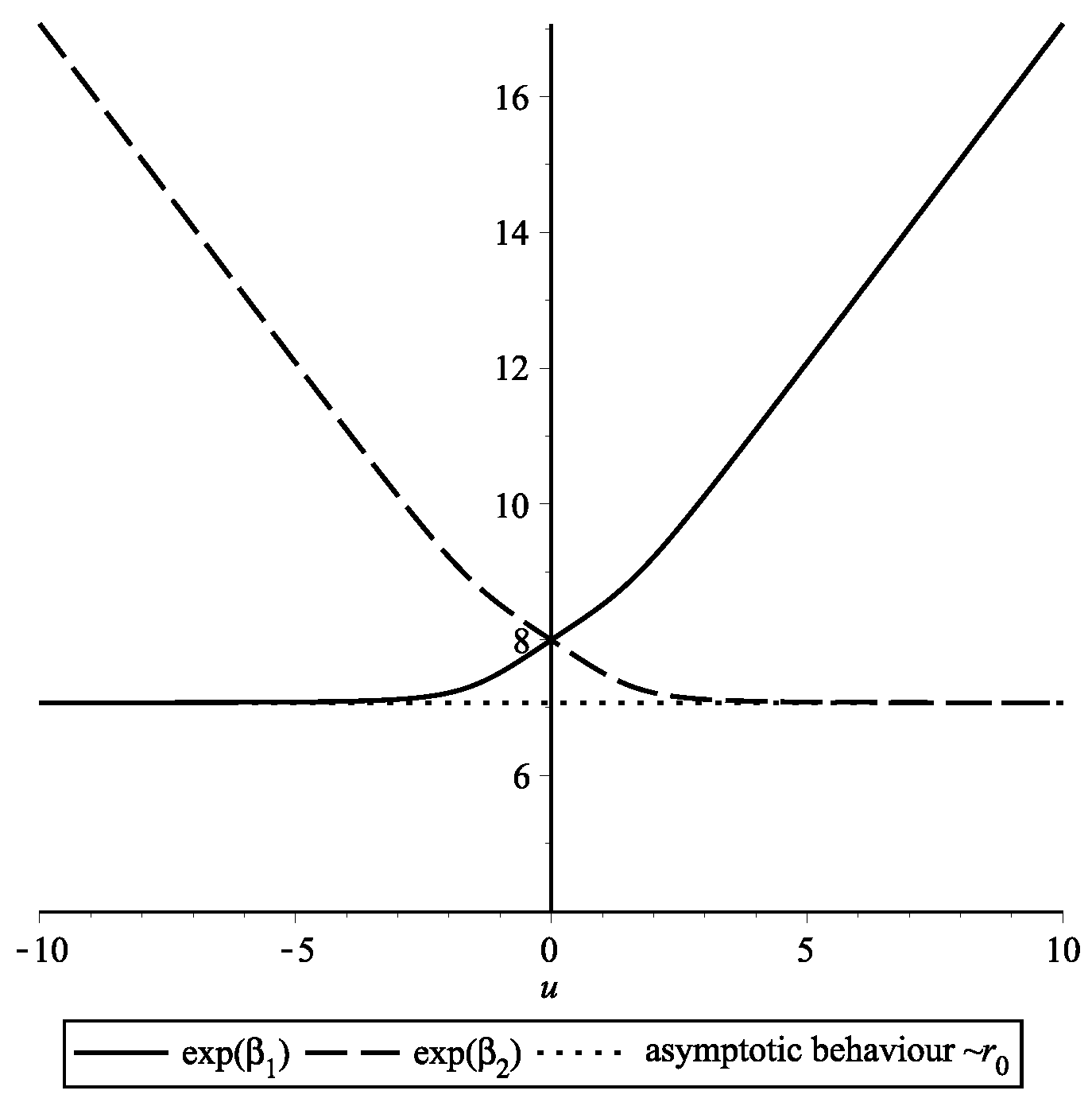
Let us study the metric that represents the transition between the domain with (large M 2 /small M 1 ) subspaces and the domain with subspaces (large M 1 /small M 2 ) [34] with the Minkowski metric at the asymptotes:
A ( u ± ) 1 ,
and
β 1 ( u + ) ln u , β 1 ( u ) ln r 0 , β 2 ( u ) ln u , β 2 ( u + ) ln r 0 .
Here, r 0 = e β c is the radius of extra space at u ± . The value of r 0 = 1 / c is connected with the physical parameter c according to Formulas (80)–(91).
For the numerical simulations, we use the Ritz method which means that the functions A ( u ) , β 1 ( u ) , β 2 ( u ) in (107) are approximated by trial functions that are chosen in the form
A ( u ) = 1 ξ 2 ξ 1 2 + u 2 ,
e β 1 ( u ) = r 0 + 1 2 u + ξ 3 4 + u 4 4 ,
e β 2 ( u ) = r 0 1 2 u ξ 3 4 + u 4 4 ,
keeping in mind conditions (109), (110). According to [35], the parameters ξ 1 , ξ 2 , ξ 3 should satisfy equation
2 ξ 2 c + ξ 1 2 ξ 2 + 3 c ξ 3 4 ( 1 4 c 2 ) + 3 c 1 ( c ) 3 / 2 ξ 3 4 = 0 .
In what follows, we consider ξ 1 , ξ 3 as independent values, and ξ 2 as their function. Parameters ξ 1 , ξ 2 , ξ 3 are to be defined by the action minimization.
Now, the action S ( ξ 1 , ξ 3 ) appears to be a function of two variables after the substitution of trial functions (111) into action (74). Classical solutions should satisfy equations
δ S δ g a b = 0
or, according to the Ritz method, [36]
S δ ξ 1 = 0 , S δ ξ 3 = 0 .
One of the ways to solve this system is to find a minimum of the auxiliary function
Ω ( ξ 1 , ξ 2 ( ξ 1 , ξ 3 ) , ξ 3 ) = S ξ 1 2 + S ξ 3 2 .
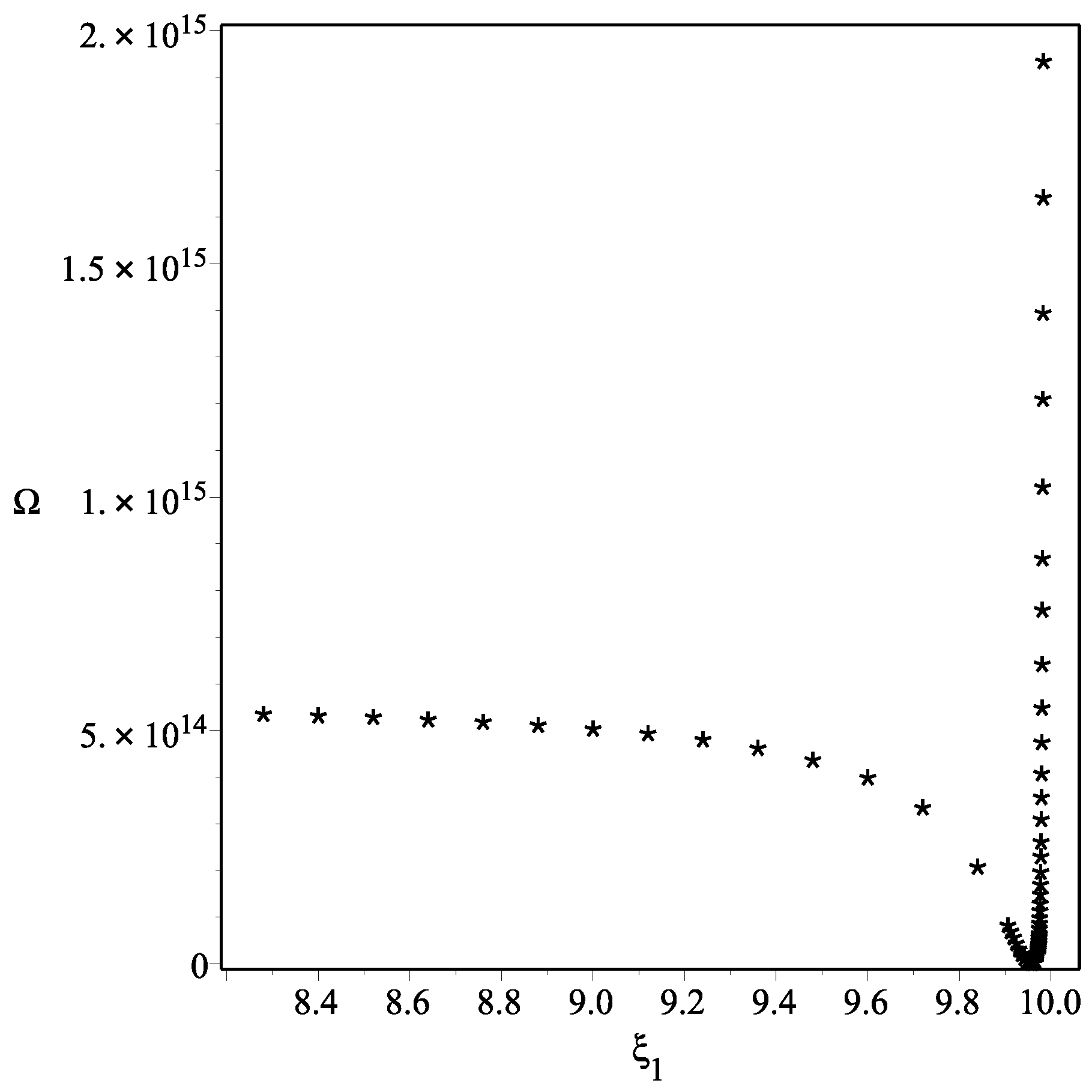
The minimization procedure for Ω ( ξ 1 , ξ 2 ( ξ 1 , ξ 3 ) , ξ 3 ) gives the minimum at ξ 1 * = 9.96 , ξ 2 * = 9.57 , ξ 3 * = 1.85 , see Figure 8. The minimum is very profound so that the trial functions, see Figure 9, are chosen properly.
For an external observer, the funnel looks like a microscopic object with the mass of the Planck scale’s order.
The method of trial functions (the Ritz method) is a useful tool to study complicated systems provided that the boundary conditions are known.

6. Conclusions

In this review, we discussed the working methods that help to cope with the mathematical difficulties of gravity with higher derivatives. All methods are supplied by examples that help to reveal the positive and negative aspects of each approach.
The method based on the conformal transformation strongly facilitates analysis in some cases, but it is mostly limited by f ( R ) models. In addition, caution in the application of this method is necessary if the quantum effects are essential.
The direct solution of the system of differential equations followed from an action minimization is a complicated problem. In addition, the progress is possible if these equations are of the second order in time derivatives. The latter is not obligatorily true for models containing invariants other than the Ricci scalar.
If the system contains a small parameter, this usually helps to obtain results. The ratio of the Ricci scalars of extra dimensions and those measured in the present Universe can be used in many models containing the extra space. It often helps to reduce a primary D-dim action with higher derivatives to the 4-dimensional action with a scalar field. The smallness of such ratio (67) should be controlled at high energies intentionally.
The trial functions method is quite universal, but the accuracy of results is not evident, and efforts should be applied to clarify the question.

Author Contributions

Conceptualization, S.G.R. and A.P.; methodology, S.G.R. and A.P.; software, S.G.R., A.P. and P.M.P.; validation, S.G.R., A.P. and P.M.P.; formal analysis, S.G.R., A.P. and P.M.P.; investigation, S.G.R., A.P. and P.M.P.; resources, S.G.R., A.P. and P.M.P.; data curation, S.G.R., A.P. and P.M.P.; writing—original draft preparation, S.G.R., A.P. and P.M.P.; writing—review and editing, S.G.R., A.P. and P.M.P.; visualization, S.G.R., A.P. and P.M.P.; supervision, S.G.R. and A.P.; project administration, S.G.R. and A.P.; funding acquisition, S.G.R. and A.P. All authors have read and agreed to the published version of the manuscript.

Funding

This research was funded by the Ministry of Science and Higher Education of the Russian Federation, Project “Fundamental properties of elementary particles and cosmology” N 0723-2020-0041. The work of A.P. and S.G.R. is performed according to the Russian Government Program of Competitive Growth of Kazan Federal University. The work of A.P. was partly funded by the Russian Foundation for Basic Research Grant No. 19-02-00496. The work of A.P was also funded by the development program of the Regional Scientific and Educational Mathematical Center of the Volga Federal District, agreement N 075-02-2020.

Conflicts of Interest

The authors declare no conflict of interest. The funders had no role in the design of the study; in the collection, analyses, or interpretation of data; in the writing of the manuscript, or in the decision to publish the results.

References

  1. Barrow, J.D.; Cotsakis, S. Inflation and the conformal structure of higher-order gravity theories. Phys. Lett. B 1988, 214, 515–518. [Google Scholar] [CrossRef]
  2. Woodard, R.P. The Theorem of Ostrogradsky. arXiv 2015, arXiv:1506.02210. [Google Scholar]
  3. Paul, B. Removing the Ostrogradski ghost from degenerate gravity theories. Phys. Rev. D 2017, 96, 044035. [Google Scholar] [CrossRef] [Green Version]
  4. De Felice, A.; Tsujikawa, S. f(R) theories. Living Rev. Relativ. 2010, 13, 3. [Google Scholar] [CrossRef] [PubMed] [Green Version]
  5. Capozziello, S.; de Laurentis, M. Extended Theories of Gravity. Phys. Rep. 2011, 509, 167–321. [Google Scholar] [CrossRef] [Green Version]
  6. Günther, U.; Moniz, P.; Zhuk, A. Multidimensional Cosmology and Asymptotical AdS. Astrophys. Space Sci. 2003, 283, 679–684. [Google Scholar] [CrossRef] [Green Version]
  7. Saidov, T.; Zhuk, A. AdS nonlinear multidimensional (D = 8) gravitational models with stabilized extra dimensions. Gravit. Cosmol. 2006, 12, 253–261. [Google Scholar]
  8. Saidov, T.; Zhuk, A. A nonlinear multidimensional gravitational model R+R-1 with form fields and stabilized extra dimensions. Astron. Astrophys. Trans. 2006, 25, 447–453. [Google Scholar] [CrossRef]
  9. Abbott, R.B.; Barr, S.M.; Ellis, S.D. Kaluza-Klein Cosmologies and Inflation. Phys. Rev. 1984, D30, 720. [Google Scholar] [CrossRef]
  10. Firouzjahi, H.; Sarangi, S.; Tye, S.H.H. Spontaneous creation of inflationary universes and the cosmic landscape. JHEP 2004, 09, 60. [Google Scholar] [CrossRef] [Green Version]
  11. Antusch, S.; Dutta, K.; Halter, S. Combining High-scale Inflation with Low-energy SUSY. JHEP 2012, 3, 105. [Google Scholar] [CrossRef] [Green Version]
  12. Khlopov, M.Y.; Rubin, S.G.; Sakharov, A.S. Primordial structure of massive black hole clusters. Astropart. Phys. 2005, 23, 265–277. [Google Scholar] [CrossRef] [Green Version]
  13. Dolgov, A.D.; Kawasaki, M.; Kevlishvili, N. Inhomogeneous baryogenesis, cosmic antimatter, and dark matter. Nucl. Phys. B 2009, 807, 229–250. [Google Scholar] [CrossRef] [Green Version]
  14. Gani, V.A.; Dmitriev, A.E.; Rubin, S.G. Deformed compact extra space as dark matter candidate. Int. J. Mod. Phys. 2015, D24, 1545001. [Google Scholar] [CrossRef] [Green Version]
  15. Dolgov, A.; Freese, K.; Rangarajan, R.; Srednicki, M. Baryogenesis during reheating in natural inflation and comments on spontaneous baryogenesis. Phys. Rev. D 1997, 56, 6155–6165. [Google Scholar] [CrossRef] [Green Version]
  16. Cline, J.M. TASI Lectures on Early Universe Cosmology: Inflation, Baryogenesis and Dark Matter. PoS 2019, TASI2018, 1. [Google Scholar]
  17. Ade, P.A.; Aghanim, N.; Armitage-Caplan, C.; Arnaud, M.; Ashdown, M.; Atrio-Barandela, F.; Aumont, J.; Baccigalupi, C.; Banday, A.J.; Barreiro, R.B.; et al. Planck 2013 results. XXII. Constraints on inflation. Astron. Astrophys. 2014, 571, A22. [Google Scholar] [CrossRef] [Green Version]
  18. Starobinsky, A.A. A New Type of Isotropic Cosmological Models Without Singularity. Phys. Lett. 1980, B91, 99–102. [Google Scholar] [CrossRef]
  19. Bamba, K.; Makarenko, A.N.; Myagky, A.N.; Nojiri, S.; Odintsov, S.D. Bounce cosmology from F(R) gravity and F(R) bigravity. J. Cosmol. Astropart. Phys. 2014, 1, 8. [Google Scholar] [CrossRef]
  20. Nojiri, S.; Odintsov, S.D.; Tretyakov, P.V. Dark energy from modified F(R)-scalar-Gauss Bonnet gravity. Phys. Lett. B 2007, 651, 224–231. [Google Scholar] [CrossRef] [Green Version]
  21. Sokolowski, L.M. Metric gravity theories and cosmology:II. Stability of a ground state in f(R) theories. Class. Quant. Grav. 2007, 24, 3713–3734. [Google Scholar] [CrossRef]
  22. Bronnikov, K.A.; Melnikov, V.N. Conformal Frames and D-Dimensional Gravity. In The Gravitational Constant: Generalized Gravitational Theories and Experiments; NATO Science Series (Series II: Mathematics, Physics and Chemistry); de Sabbata, V., Gillies, G.T., Melnikov, V.N., Eds.; Springer: Dordrecht, The Netherlands, 2004; Volume 141. [Google Scholar] [CrossRef] [Green Version]
  23. Faraoni, V.; Gunzig, E.; Nardone, P. Conformal transformations in classical gravitational theories and in cosmology. Fundam. Cosm. Phys. 1999, 20, 121–175. [Google Scholar]
  24. Blanco-Pillado, J.J.; Burgess, C.P.; Cline, J.M.; Escoda, C.; Gomez-Reino, M.; Kallosh, R.; Linde, A.; Quevedo, F. Racetrack Inflation. J. High Energ. Phys. 2004, 11, 63. [Google Scholar] [CrossRef]
  25. Kirillov, A.A.; Korotkevich, A.A.; Rubin, S.G. Emergence of symmetries. Phys. Lett. 2012, B718, 237–240. [Google Scholar] [CrossRef] [Green Version]
  26. Burgess, C.P. An Introduction to Effective Field Theory. Annu. Rev. Nucl. Part. Sci. 2007, 57, 329–362. [Google Scholar] [CrossRef] [Green Version]
  27. Bronnikov, K.A.; Rubin, S.G. Self-stabilization of extra dimensions. Phys. Rev. 2006, D73, 124019. [Google Scholar] [CrossRef] [Green Version]
  28. Donoghue, J.F. General relativity as an effective field theory: The leading quantum corrections. Phys. Rev. 1994, D50, 3874–3888. [Google Scholar] [CrossRef] [Green Version]
  29. Bronnikov, K.A.; Konoplich, R.V.; Rubin, S.G. The diversity of universes created by pure gravity. Class. Quant. Grav. 2007, 24, 1261–1277. [Google Scholar] [CrossRef]
  30. Bronnikov, K.; Rubin, S.; Svadkovsky, I. Multidimensional world, inflation and modern acceleration. Phys. Rev. D 2010, 81, 084010. [Google Scholar] [CrossRef] [Green Version]
  31. Fabris, J.C.; Popov, A.A.; Rubin, S.G. Multidimensional gravity with higher derivatives and inflation. Phys. Lett. B 2020, 806, 135458. [Google Scholar] [CrossRef]
  32. Shinkai, H.A. Truncated post-Newtonian neutron star model. Phys. Rev. D 1999, 60, 067504. [Google Scholar] [CrossRef] [Green Version]
  33. Boehmer, C.; Harko, T. Dynamical instability of fluid spheres in the presence of a cosmological constant. Phys. Rev. D 2005, 71, 084026. [Google Scholar] [CrossRef] [Green Version]
  34. Rubin, S.G. Interpenetrating subspaces as a funnel to extra space. Phys. Lett. B 2016, 759, 622–625. [Google Scholar] [CrossRef] [Green Version]
  35. Lyakhova, Y.; Popov, A.A.; Rubin, S.G. Classical evolution of subspaces. Eur. Phys. J. 2018, C78, 764. [Google Scholar] [CrossRef]
  36. Gander, M.J.; Wanner, G. From Euler, Ritz, and Galerkin to Modern Computing. SIAM Rev. 2012, 54, 627–666. [Google Scholar] [CrossRef] [Green Version]
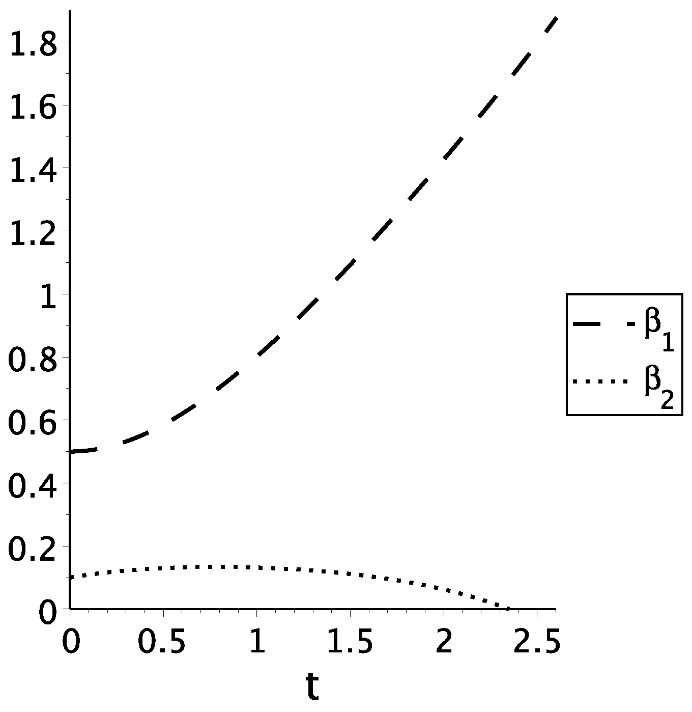
Figure 1. Numerical solution of (19), (20) and (22) for d 1 = d 2 = 3 , β 1 ( 0 ) = 0.5 , β ˙ 1 ( 0 ) = 0 , β 2 ( 0 ) = 0.1 , β ˙ 2 ( 0 ) = 0.5 , R ˙ ( 0 ) = 0 . R ( 0 ) 12.67452 is found from Equation (23).
Universe 06 00187 g001
Figure 2. The same as in Figure 1 except β ˙ 2 ( 0 ) = 0.1 .
Universe 06 00187 g002
Figure 3. Solution for the system (50) with the initial conditions (53) and (55).
Universe 06 00187 g003
Figure 4. Numerical solution to the system of Equations (63)–(65) for initial conditions α ( 0 ) = 7 , α ˙ ( 0 ) = 1 , β ( 0 ) = 4 , β ˙ ( 0 ) = 0 , R ˙ ( 0 ) = 0 . The initial condition R ( 0 ) 11.999 is found from Equation (66). The Lagrangian parameters are a = 200 , c = 0.001 , k = 500 .
Universe 06 00187 g004
Figure 5. Numerical solution to the system of Equations (63)–(65) for initial conditions α ( 0 ) = 15 , β ( 0 ) = 2 , α ˙ ( 0 ) 0.404667 , β ˙ ( 0 ) = 0 , R ˙ ( 0 ) = 0 . R ( 0 ) 2.09126 is found from Equation (66). The Lagrangian parameters are a = 2.77 , c = 0.49 , k = 2.98 .
Universe 06 00187 g005
Figure 6. Numerical solution to the system of Equations (63)–(65) for initial conditions α ( 0 ) = 15 , α ˙ ( 0 ) 0.40467 , β ( 0 ) = b c 1.99303 , β ˙ ( 0 ) = 0 , R ˙ ( 0 ) = 0 . R ( 0 ) 2.0765 is found from Equation (66). For the found numerical solution, a = 2.77 , c = 0.49 , k = 2.98 .
Universe 06 00187 g006
Figure 7. The form of the potential (left) and kinetic term (right) for the parameters n = 2 , b = 1 , a = 2 , c V = 8 , c K = 15000 . The potential minimum is in the point ϕ m 0.083 , m D = 1 .
Universe 06 00187 g007
Figure 8. Auxiliary function Ω vs. the minimization parameter ξ 1 for ξ 2 * = 9.57 , ξ 3 * = 1.85 and f ( R ) -parameters a = 2 , b = 1 , c = 0.02 . The minimum of Ω corresponds to ξ 1 * = 9.96 . Ω ( ξ 1 * = 9.96 , ξ 3 * = 1.85 ) = 5.3 × 10 11 .
Universe 06 00187 g008
Figure 9. Radii of two-dimensional subspaces vs. the Schwarzschild radial coordinate u for parameter values a = 2 , b = 1 , c = 0.02 , ξ 3 = 1.85 .
Universe 06 00187 g009
Publisher’s Note: MDPI stays neutral with regard to jurisdictional claims in published maps and institutional affiliations.