Article

Kerr Black Holes within a Modified Theory of Gravity

by
Peter O. Hess
1,2,* and
Enrique López-Moreno
3
1
Instituto de Ciencias Nucleares, Universidad Nacional Autónoma de México, Ciudad de México 04513, Mexico
2
Frankfurt Institute for Advanced Studies, J.W. von Goethe University, 60323 Hessen, Germany
3
Facultad de Ciencias, Universidad Nacional Autónoma de México, Ciudad de México 04510, Mexico
*
Author to whom correspondence should be addressed.
Universe 2019, 5(9), 191; https://doi.org/10.3390/universe5090191
Submission received: 6 July 2019 / Revised: 16 August 2019 / Accepted: 24 August 2019 / Published: 28 August 2019
(This article belongs to the Special Issue Rotation Effects in Relativity)

Abstract

:
The Kerr black hole is studied within a modified theory of gravity, which adds the effects of vacuum fluctuations near a black hole. These vacuum fluctuations are treated as a dark energy. A parameter is introduced to account for these fluctuations. It is zero for the standard theory and acquires a maximal value, just before there would be no event horizon. The existence of an event horizon not only depends on the value of this parameter, but also on the spin of the black hole. In addition, we study the existence of a light-ring. We also elaborate on the relation of the appearance and vanishing of the event horizon and light-ring to phase transitions.

1. Introduction

The General Relativity (GR) is one of the best tested theories [1]. Recently, the detection of gravitational waves [2] and the first optical resolution of the black hole in M87 [3,4,5,6,7,
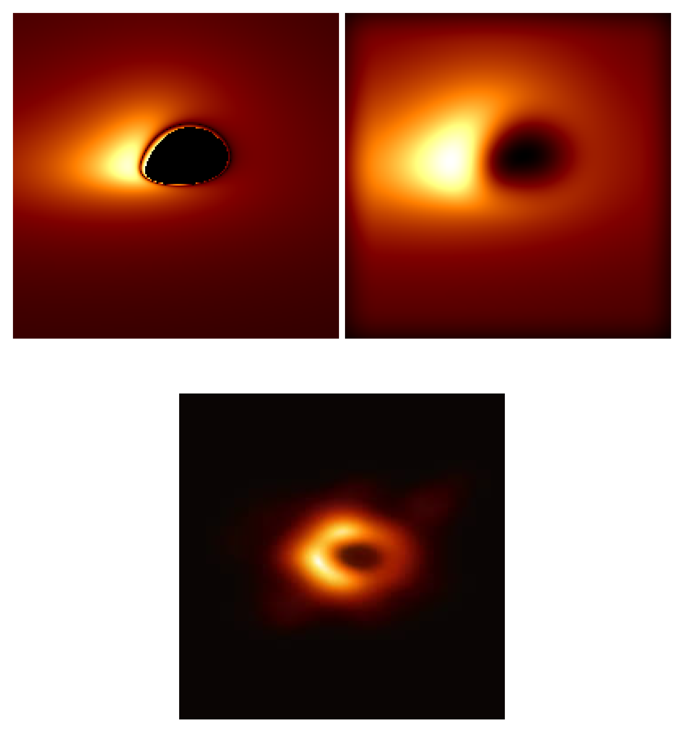
8] are all consistent with GR, i.e., one observes a shadow of the black hole. The size of it can be understood within GR and its radius is about 3 m 0 . Unfortunately, the resolution is only of 24 μ a s , which will smooth detailed structures, which are predicted by us (see the discussion in the main body of the text).
There are some concerns that, for strong gravitational fields, compared to the solar system, modifications to GR probably have to be applied. This did lead to several attempts to modify GR, which will be all resumed briefly in the next section. Here, we will concentrate on the so-called pseudo-complex General Relativity (pc-GR).
A complete review on the pc-GR, its motivation and relations to other approaches can be found in the book by Hess, Schäfer and Greiner [9]. The mathematics of the pc-GR is explained in the first and last chapter of the book, using differential geometry. Information on this can also be found in [10]. The pc-GR was first proposed in [11]. A general formulation, besides in [9], can also be found in [12,13], where, in [12], circular stable orbits were investigated and the last stable orbits, compared to GR. One important result is that, for small a, the last stable orbit in pc-GR is a little bit closer to the black hole than in GR. From a limiting value of a on, stable orbits up to the surface of the star exist. In this review, we will elaborate on the consequences of it. The theory predicts a different behavior of an accretion disc near the black hole, showing a dark ring followed by a bright one further in. Studies on this were also published in [14,15] and more recently in [16,17]. The main feature is the ring structure, mentioned above, which is quite independent from the mass of the black hole and the type of the accretion disc (if it is thin, thick, a torus, ...), save that the positions of the structures scale with the mass. The intensities of the light emission are larger in pc-GR than in GR (see also the discussion in the main body of this review).
In addition, neutron stars were studied in [18,19,20], in addition to [9]. Including the effects of the pc-GR, stars up to six solar masses were obtained in [18,20] and up to 200 solar masses in [19].
Cosmological models were investigated in [21,22], which agree with current observations, but with different outcomes in the far future. Due to many parameters, the predictive power is rather limited. Except for a big rip, possibilities were found that the universe approaches a constant acceleration, or approaches to zero acceleration, or it can collapse again. There are different approaches to study future outcomes (see, for example [23,24], where possible future evolutions of the universe are investigated, using a thermodynamic approach). Though interesting and worth mentioning, it differs from the path taken in pc-GR. It would be interesting in the future to connect both approaches, i.e., to consider the thermodynamic approach in pc-GR. Another proposal could be that the authors of [23,24] use the modified metric of pc-GR.
Gravitational waves were considered in pc-GR: in [25], the gravitational wave event GW150914 was treated within pc-GR, with the result that probably the masses and distances involved are larger; however, a very simple model was used. The main reason for this behavior is that the orbital frequency becomes very small when the two masses in a black hole merger approach each other and, in order to obtain the observed frequencies, larger masses are required. In [26], the axial and polar modes of the ring down phase were calculated, however, with some problems of convergence, due to the method used for solving the differential equation. All, except for the discussion of gravitational waves, are neatly summarized in [9].
The main motivation for the development of pc-GR was to investigate what kind of theory emerges when the coordinates are algebraically extended (where only the pseudo-complex extension makes sense, as will be discussed further below): Is there a possibility to avoid the event horizon? What are the observable effects (particles in a circular orbit, behavior of accretion discs, position of the light-ring, neutron stars, etc.)? As we will point out in the next section, a minimal length element parameter may be involved. What is its effect? Are there consequences or at least suggestions for quantum effects in gravity? Not all has been answered up to now, due to mathematical problems, but most of the above questions have been treated.
Up to now, the main parameter ( b n , see main body of the text) of the theory was chosen such that no event horizon appears. For b n = 0 , the standard GR is recovered. In this review, we will not cover all aspects of the theory (please also consult [13]), but it would be interesting to vary the parameter b n from 0 to the value, from which no event horizon appears, as done also in [27,28] for gravitational waves. In this manner, the GR and pc-GR can be connected smoothly. One can also study the behavior of the event horizon and the light-ring as a function in the rotational parameter a and b n .
The description is completely classical, though a dark energy contribution will be introduced in a classical language.
In Section 2, the motivation for the algebraic extension of GR is described in more detail and the structure of pc-GR is discussed. The modified metric of a rotating star is listed (Kerr solution) and the corresponding Einstein equations are presented. In Section 3, various consequences and structural changes are considered. The condition for the existence of an event horizon and a light-ring depends on a parameter ( b n ), introduced in a phenomenological manner, which varies from zero (GR) to a maximal value (pc-GR). Structural changes, related to phase transitions, can be described within the theory of catastrophes [29]. The difference in structure (between GR and pc-GR) of an accretion disc around a black hole is also presented, important for the comparison to the observational data. One recent big advance in this direction was reported by the Event Horizon Telescope Collaboration [3,4,5,6,7,8], where, for the first time, the black hole shadow of M87 was resolved. These references contain a huge amount of information, still to be analyzed. We also will compare some of the results to the recent observation of a black hole [3,4,5,6,7,8] and if one can distinguish pc-GR from GR. This part represents new results.
In Section 4, conclusions are drawn.
We use the signature ( + + + ) for the metric. Furthermore, the light velocity c and the gravitational constant are set to one (i.e., c = G = 1 ).

2. The Modified Theory: Pseudo-Complex General Relativity

At first, a historical overview on attempts to extend the GR is given, in addition to the reasons for it and why we decided for the pc-GR:
Extensions of the GR have been discussed several times in the past: Einstein extended the metric to a complex one [30,31], in an attempt to unify GR and the Electro-Magnetism. He defined a complex metric
G μ ν = g μ ν + i F μ ν , G μ ν * = G ν μ ,
where the real part is the standard metric of GR and the imaginary part is the electromagnetic tensor. The real part is symmetric while interchanging the indices and the imaginary part is anti-symmetric. This can be seen as follows:
G μ ν * = g μ ν i F μ ν = G ν μ = g ν μ + i F ν μ .
Comparing both sides leads to
g μ ν = g μ ν and F μ ν = F ν μ .
Why a complex extension did not work will become obvious in a moment.
The motivations of Born [32,33] were quite different. His concern is that, in Quantum Mechanics, the coordinates and momenta are treated on an equal footing. Canonical transformations of all kinds are allowed, which leave the commutation relations invariant, and one can even interchange coordinates and momenta. On the contrary, in GR, the coordinates play a singular role—in the length element square, only coordinates appear. He tried to recover the symmetry between the coordinates and momenta, leading to a modification of the length element, including momentum dependent terms, however, with the price of a mass dependence on a particle. The attempt by Born was retaken by Caianiello [34], who introduced in the length element squared an infinitesimal quadratic 4-velocity term, without the reference to a particle, implying an infinitesimal length scale, equivalent to a maximal acceleration:
d ω 2 = g μ ν d x μ d x ν + l 2 d u μ d u ν .
The l is a length parameter and is not subject to a Lorentz (or Poincaré) transformation. Thus, Lorentz invariance is guaranteed with an infinitesimal length scale in the model! Extracting an eigentime d τ 2 , taking into account that d u μ d τ is an acceleration a μ and using that η μ ν a μ a ν = a 0 a 0 a i a i = a 2 ( η μ ν is the Minkowski metric), we obtain d ω 2 = 1 l 2 a 2 g μ ν , i.e., it corresponds to a new metric G μ ν = 1 l 2 a 2 g μ ν . The acceleration is then limited by a 1 l 2 .
We will see that these modifications are included in pc-GR in a particular limit. A more detailed resume on former intentions to extend the GR is given in [9].
In [35], all kinds of algebraic extensions of the coordinates were considered and the field equations for weak gravitational fields were obtained. It was shown that nearly all algebraic extensions contain solutions for tachyons or ghosts, which shows that nonphysical solutions appear. Only real and pseudo-complex (called in [35] hyper-complex) coordinates did not have this problem. This is the reason why we discuss only this particular extension:
In pc-GR, the coordinates of GR are extended to these so-called pseudo-complex (pc) variables:
X μ = x μ + I y μ ,
( μ = 0 , 1 , 2 , 3 ), with I 2 = 1 , which justifies its name (though the name is not universal in the literature, where these variables are denoted as para-complex, etc.). The complex conjugate is defined as X * μ = x μ I y μ . In [34], the variable y μ is proportional to a minimal length scale, l, multiplied by the 4-velocity component u μ . It is important to stress that the parameter l is not a physical length and, thus, is not effected by a Lorentz transformation. Unfortunately, the relation of y μ to the 4-velocity is only correct in flat space, where the constraint used further below in (9) reduces to the standard dispersion relation g μ ν y μ d y ν = 0 , with the solution y μ u μ . The minimal length parameter l is required as a factor by dimensional considerations. When the space is not flat, no easy solution has been found yet, but, in principle, can be found by solving the constraint (9).
An important nature of these variables is revealed when we change to the basis
X μ = X + μ σ + + X μ σ σ ± = 1 2 1 ± I ; σ + σ = 0 .
It implies that there are variables of the type v σ ± that have a zero norm. Thus, the variables form a ring and not a field. The components of σ ± are called zero divisor components.
The division into the zero divisor components can be done for any pc-function F ( X ) = F ( X + ) σ + + F ( X ) σ . Mathematical manipulations are independent from each other (see also [9]).
The fact that σ + σ = 0 allows for formulating in each zero-divisor component a theory of General Relativity! In order to get a consistent theory, both zero-divisor components have to be connected. In [9,11], this is done introducing a modified variational principle, where the variation of the action is proportional to a “general zero”, i.e., a function with a zero norm. However, this is not necessary: in [36] and the last chapter of [11], it is shown that a constraint can be implemented and a usual variational principle leads to modified Einstein equations. In what follows, we will resume the main steps.
The constraint requires that the pc length element
d ω 2 = g μ ν ( X ) d X μ d X ν = g μ ν + ( X + ) d X + μ d X + ν σ + + g μ ν ( X ) d X μ d X ν σ + = g μ ν S d x μ d x ν + d y μ d y ν + g μ ν A d x μ d y ν + d y μ d x ν + I g μ ν A d x μ d x ν + d y μ d y ν + g μ ν S d x μ d y ν + d y μ d x ν
is real. We used the definitions
g μ ν S = 1 2 g μ ν + + g μ ν , g μ ν A = 1 2 g μ ν + g μ ν .
In addition, the representation of d 2 ω in the zero-divisor is indicated and in the original basis ( ( 1 , I ) -basis). (7) coincides with the one of [34], when y μ is substituted by l u μ . In each component of the zero divisor basis, only Riemannian manifolds are considered, thus other types of manifolds are not included yet.
Setting the pseudo-imaginary part to zero leads to the constraint
g μ ν + ( X + ) d X + μ d X + ν g μ ν ( X ) d X μ d X ν = 0 .
The action, without the constraint, is given by
S = d x 4 g R + 2 α ,
where R is the Riemann scalar. The last term in the action integral allows for introducing the cosmological constant in cosmological models, where α has to be constant in order not to violate the Lorentz symmetry. This, however, changes when a system with a uniquely defined center is considered, which has spherical (Schwarzschild) or axial (Kerr) symmetry. In these cases, the α is allowed to be a function in r, for the Schwarzschild solution, and a function in r and ϑ , for the Kerr solution.
The variation is independent in each zero-divisor basis. The result is the set of the modified Einstein equations (see [36])
R μ ν ± 1 2 g μ ν ± R ± = 8 π T ± μ ν Λ ,
with
8 π T ± μ ν Λ = λ u μ u ν + λ y ˙ μ y ˙ ν ± u μ y ˙ ν ± u ν y ˙ μ + α g μ ν ± .
The energy-momentum tensor corresponds to the one of an asymmetric ideal fluid. The y μ is related to the appearance of a minimal scale, as explained in the case of the proposal given in [34]. Because these effects are practically impossible to measure due to their smallness, it suffices to restrict to the real part of the equations, which leads to the only one equation:
R μ ν 1 2 g μ ν R = 8 π T μ ν Λ .
The energy-momentum tensor acquires under this approximation the form
T μ ν , R Λ = ( ϱ Λ + p ϑ Λ ) u μ u ν + p ϑ Λ g μ ν + p r Λ p ϑ Λ k μ k ν , .
The relations to the parameter in the action are (see [36])
λ = 8 π λ ˜ , α = 8 π α ˜ , λ ˜ = p ϑ Λ + ϱ Λ , α ˜ = p ϑ Λ , λ ˜ y μ y ν = p r Λ p ϑ Λ k μ k ν ,
where k μ are the components of a space-like vector, orthogonal to the 4-velocity.
Because we do not know the exact solution for y μ , we cannot derive the exact form of the energy- momentum tensor and, thus, we are left to propose a phenomenological model. The energy-momentum tensor describes an ideal anisotropic fluid. That it has to be anisotropic is explained in [9]: First of all, as explained further below, the energy-momentum tensor on the right-hand side of the Einstein equations is assumed to be related to the contribution of vacuum fluctuations, which represents a dark energy. This dark energy can be calculated within the one-loop approximation of GR as described in [37] and done in [38]. The equation of state of a dark energy in the radial pressure is p r Λ = ρ Λ , where p r Λ is its pressure and ρ Λ is the dark energy density. Within the Tolmann–Oppenheimer–Volkoff (TOV) equations, the radial derivative of the pressure is proportional to the sum of the radial pressure (which is equal to the tangential one in case of an isotropic fluid) and the density, i.e., it is zero. An anisotropic fluid is characterized by an addition term, proportional to the difference of the radial and tangential pressure ( p θ Λ ). Without this term, the radial derivative of the pressure is zero and thus constant in r. Because of the proportionality of the energy density to the pressure, this also implies a constant energy density. Requiring that the density has to vanish at infinity results in a zero density, contrary to the requirement that the density is building up toward smaller distances. Only an anisotropic fluid can resolve this contradiction (see [9]).
In the absence of a quantized theory of gravity, it is impossible to deduce, for example, the radial dependence of the dark-energy density. Here, we rely on information from one-loop calculations in GR [37], which where performed in [38] for a static Schwarzschild back-ground metric. In [38], the energy density rises proportional to 1 / r 6 1 2 m 0 r 2 toward the center, i.e., it is singular at the Schwarszschild radius. Clearly, the assumption of a static metric fails when the gravitational field increases too much. In this case, one has to include back-reaction effects, which is very difficult to do. This tells us that the fluctuations increase toward the center and they can become large. To avoid the singularity at the Schwarzschild radius, we propose a phenomenological model, where the dark-energy density is treated classically and behaves as
ϱ Λ B n r n + 2 ,
where, in a first attempt, n = 3 was taken. It is strong enough in order not to contribute to the known observations within the solar system and other systems with not too strong gravitational fields [1]. There may be other dependencies with n > 3 and, in fact, in [27,
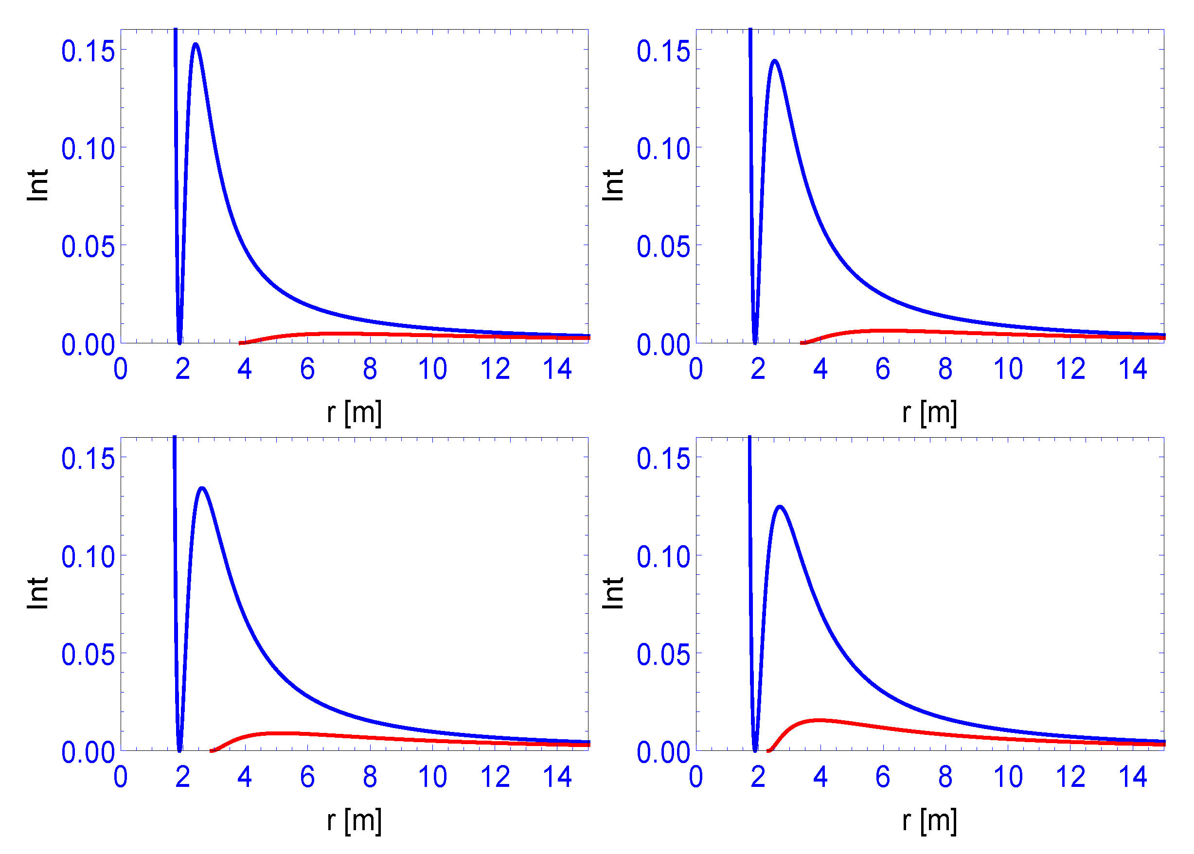
28], it was shown that the fall-off of the dark-energy density has to be stronger. We will discuss other cases of the fall-off, ordered by a number n as in (16); however, the main conclusions and structural predictions of the theory remain similar.
In [12], the pc-Kerr solution was derived and here we list it for any n
g 00 = r 2 2 m 0 r + a 2 cos 2 ϑ + B n ( n 1 ) ( n 2 ) r n 2 r 2 + a 2 cos 2 ϑ , g 11 = r 2 + a 2 cos 2 ϑ r 2 2 m 0 r + a 2 + B n ( n 1 ) ( n 2 ) r n 1 , g 22 = r 2 + a 2 cos 2 ϑ , g 33 = ( r 2 + a 2 ) sin 2 ϑ + a 2 sin 4 ϑ 2 m 0 r B n ( n 1 ) ( n 2 ) r n 2 r 2 + a 2 cos 2 ϑ , g 03 = a sin 2 ϑ 2 m 0 r + a B n ( n 1 ) ( n 2 ) r n 2 sin 2 ϑ r 2 + a 2 cos 2 ϑ .
The a is the spin parameter in units of m 0 . The solution is identical to the standard Kerr solution, except for the term B n ( n 1 ) ( n 2 ) r n 2 . The m 0 is the mass value observed at infinite distance and occasionally it will be abbreviated in the figures simply by m, clear from the context.
The B n is given by
b n m 0 n = B n > 2 ( n 1 ) ( n 2 ) n 2 ( n 1 ) n n 1 m 0 n = b n max m 0 n .
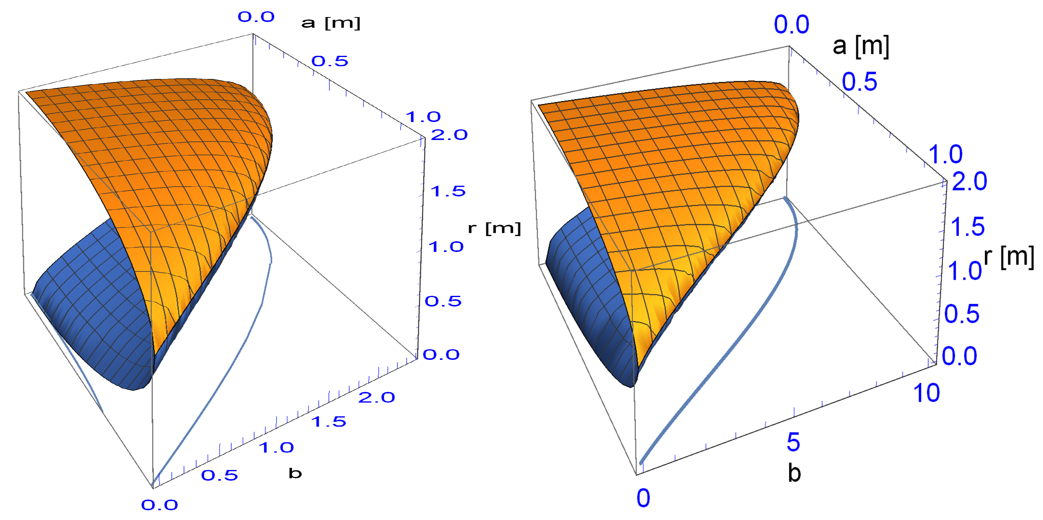
For the equal sign, an event horizon is located at
r h = 2 ( n 1 ) n m 0 .
In this contribution, some examples are calculated with n = 3 or n = 4 and we will vary the parameter b n in B n = b n m 0 n from zero to a maximal value 64 27 for n = 3 and 81 8 for n = 4 . For a larger value, there is no event horizon present anymore. We will also vary the spin-parameter a from zero to m 0 and show that, already for b n 0 , there is a region of large a values where this horizon disappears. For example, the question is, if there is or is not an event horizon already becomes relevant for tiny admixtures of vacuum fluctuations! This is similar, but not equal, to the so-called naked singularities: First, there is no singularity within the pc-GR and, second, what is exposed is the surface of a star. However, seeing the surface will be very difficult because the red-shift tends to infinity.
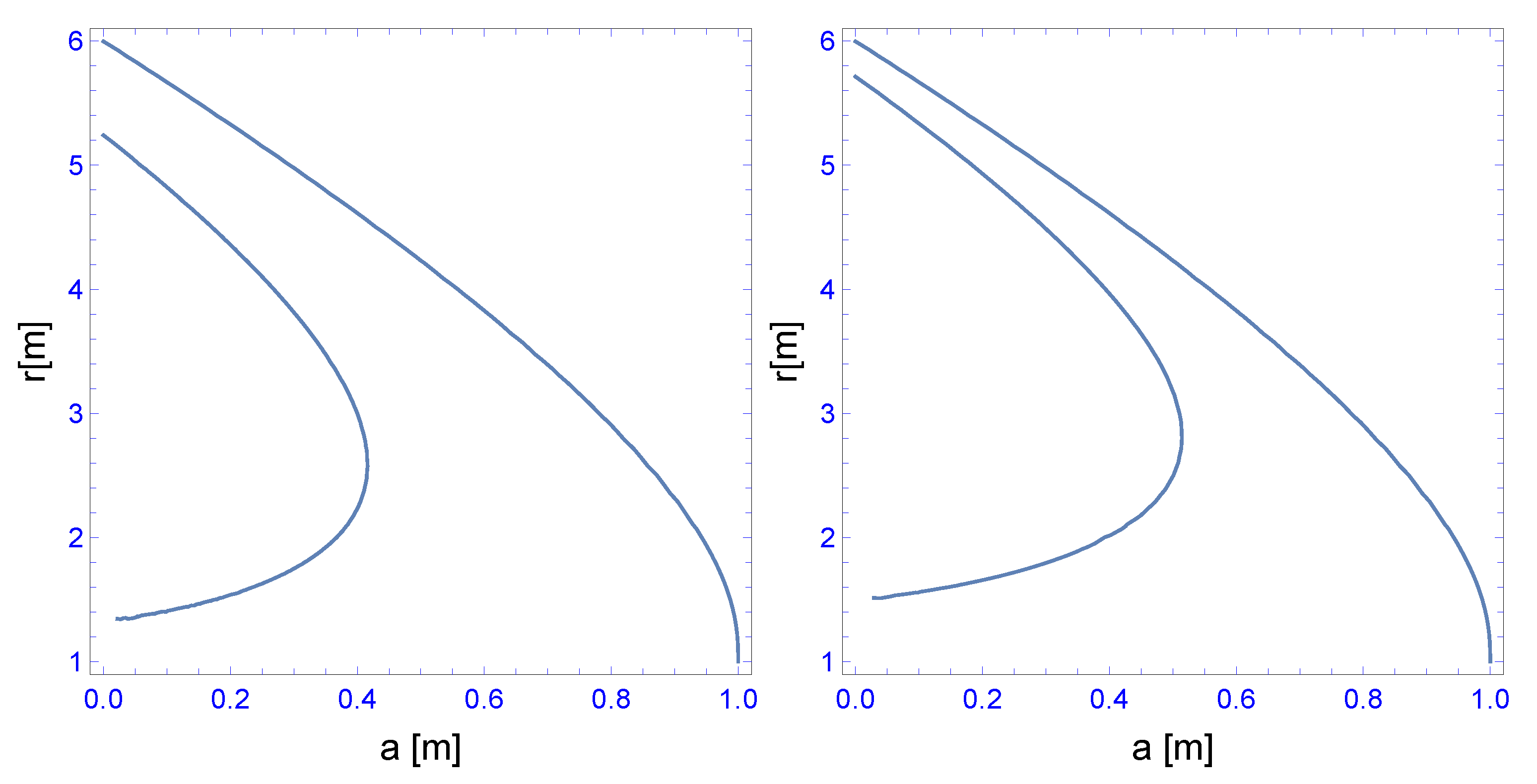
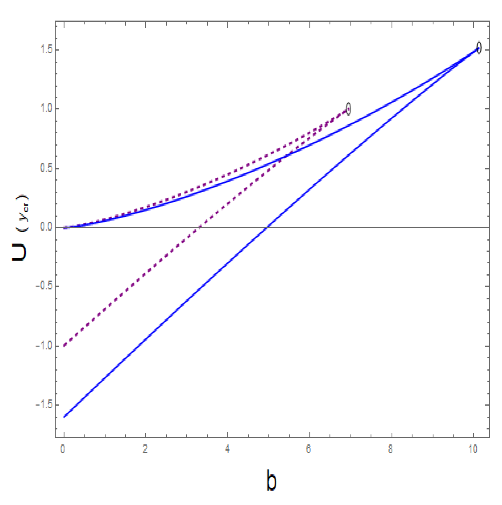
Another topic will be the calculation of the position of the light-ring. A light-ring is defined as the geodesic of a photon in a circular orbit ( r = const). In GR, there is, for a = 0 , only one light-ring at r = 3 m 0 and the value is slightly lowered for larger a. In contrast, in pc-GR and, for values b n > 0 , the structure becomes quite involved. We will investigate this property and relate it to phase transitions, using the Catastrophe Theory [29].
The application of pc-GR is not only limited to the region outside of a mass distribution, but also was applied to the interior of the star [18,19,39,40,41,42,43]. The main problem is to propose a coupling of the dark energy to the mass distribution, which, due to not knowing it from first principles, is always charged with phenomenological assumptions. In [18], a linear relation was assumed, which, however, leads to an upper limit of six solar masses for a star. The reason is that, near the surface, the repulsion is strong enough that the star sheds its upper parts of the surface. In [19], this was resolved partially, applying a calculation within the one-loop approximation of quantized gravity [37] and using the monopole approximation. As a result, the distribution of the dark energy turns out to fall off stronger near the surface. With that, stars with up to 200 solar masses were found to be stable. This already indicated that any mass of a star can probably be stabilized, i.e., even the large masses in the center of galaxies of billions of solar masses are stable and rather dark stars than black holes. There are different, alternative, approaches, e.g., in [39,40,41,42,43] compact and dense objects were investigated within the pc-GR and maximal masses were also deduced.

3. Event Horizons and Light-Rings: Phase Transitions

All of the following results were obtained partly with the help of the MATHEMATICA, version 11.3.0.0. (WOLFRAM, Champaign, IL,U.S.A.) [44]. The notebook files of MATHEMATICA can be retrieved from [45].

3.1. Circular Orbital Motion

The infinitesimal length square element d ω 2 in terms of the metric components is given by
d ω 2 = g 00 d t 2 + 2 g 11 d r 2 + g 22 d ϕ 2 + g 33 d θ 2 + 2 g 02 d ϕ d t ,
with the metric components listed in (17).
Circular orbital motion is defined by r ˙ = d r d τ = 0 , where d τ is either the infinitesimal difference of the eigentime or the length element d ω . The particle moves on a geodesic path and the deduced frequency is given by [17]
ω n = 1 a + 2 r h n ( r ) , h n ( r ) = 2 r 2 n B n ( n 1 ) ( n 2 ) r n + 1 .
In [46], the orbital motion frequency of a particle in a prograde circular orbit (assumed here) was deduced, using the method of an effective potential. In addition, the motion of a photon in a circular orbit is deduced, which satisfies, in addition, d ω 2 = 0 .
The approach presented here is different from [47], where the path of a particle following a gravitational collapse of a star is investigated, including a semi-quantum mechanical description of the particle. Although it is very interesting, it would lead here to a too extensive discussion, out of the scope of this article, also requiring adding a complete new description to the problem. It should, however, be useful to discuss a collapsing star within pc-GR. One first step is to change the metric used in [47] to the modified metric in pc-GR.
The orbital frequency of a particle in its prograde orbit is shown in Figure 1, for a = 0.9 m 0 and n = 3 , n = 4 , where the b n values are 64 27 for n = 3 and 81 8 for n = 4 . The upper curve is the result of GR while the two lower ones are for n = 3 and n = 4 in pc-GR. The maximum is at
r ω max = n ( n + 2 ) b n max 6 ( n 1 ) ( n 2 ) 1 n 1 m 0 ,
independent froma. In case b = b n max , there is a zero of the orbital frequency, coinciding with a horizon (19), and it is also independent on a. r 0 is at the estimated position of the star’s surface. For 0 b n < b n m a x , the lower curves slowly merge into the upper one for b 0 .
The stable orbits are defined in terms of a saddle point of the effective potential, see [9,14], and they are plotted in Figure 2. The left panel shows the region of stable orbits in GR and pc-GR for n = 3 , while the right shows the region of stable orbits for GR and pc-GR for n = 4 (see also the figure caption for explanation). When n increases, for small a, both curves, GR and pc-GR, approach each other. However, the curve in pc-GR starts at a = 0 at smaller distances to the black hole than GR.
The light emission from a disc is calculated using the 2014 version of the GYOTO routines [48], which uses the raytracing method and also allows for changing the metric input. Because the last stable orbit reaches further in, more gravitational energy is released and light emission increases. This can be verified in Figure 3, where simulations of thin accretion discs are presented for a = 0.9 m 0 , using the model of [49]. The left panel is pc-GR for a = 0 , being similar in structure to GR but with a greater intensity, and the right panel for a = 0.9 m 0 , which now shows a dark ring followed further in by a bright ring. In Figure 4, the simulations are shown for the same type of disc, but for different n. The left figure refers to n = 3 and the right one to n = 4 . When n is increased, the position of the dark and bright rings are shifted to larger r values. In fact, the parameter n can be determined through (21) and measuring the position of the dark ring, which gives the maximum of the frequency.
This behavior is understood by inspecting Figure 1: at the maximum of the orbital frequency, neighboring orbitals are very similar and friction is low, such that the disc gets less excited and a dark ring forms. Above and below the maximum, the change in orbital frequency for neighboring orbitals increases and friction is high, which results in a larger excitation and the light emission increases. In this sample calculation, the orientation of the accretion disc relative to the observer is 80 . However, these studies require a resolution of at least 0.5 μ a s , not yet reached by the EHT. In the upper row of Figure 5, simulations of an accretion disc are shown, with a large resolution (left) and a low resolution (right). The inclination of the disc with respect to the observer is now 70 and a = 0.6 . Below these figures, the EHT result is copied from [3] and rotated by 90 .
In Figure 6, we compare the simulation of an accretion disc in GR (left panel) with the one in pc-GR (right panel), assuming a resolution of 20 μ a s , as reported by the EHT-collaboration. As can be seen, the resolution is too low for detecting significant structural differences. This probably also affects other extensions of GR, i.e., the EHT results make it difficult to discriminate alternative theories.
The flux of light emitted by a thin disc, discussed in the above simulations, is determined as explained in [14,49] (please consult these references for more detailed information). The formula used is
f = ω r E ω L z 2 rms r E ω L z L z r d r ,
where ω r is the derivative in r of the circular orbital frequency, L z is the orbital angular momentum, with L z r its derivative in r and E is the orbital energy. The lower limit rms = r ω max is the position of the maximum of the orbital frequency. As shown in [14], the integral yields only positive values. The origin of the flux is in the friction between neighboring orbitals and it is distributed from orbitals of larger frequencies to orbitals with lower frequencies.
In Figure 7, we plot the distribution of emitted intensities as a function in r, comparing pc-GR (upper curves) with GR (lower curves), as a function in a. In the upper row left panel, it starts at a = 0.6 m 0 and ends in the second line, right panel, at a = 0.9 m 0 , applying steps of 0.1 m 0 . The intensities in pc-GR turns out to be significantly larger than in GR. The peak emission in pc-Gr is at approximately r = 3 m 0 , with little variation. The peak of emission in GR, on the other hand, starts at 6 m 0 for a = 0.6 m 0 and end at approximately 4 m 0 for a = 0.9 m 0 . The results in pc-GR are more in line with the observation, reporting the peak at about 3 m 0 .

3.2. Event Horizons

In this section, we discuss the dependence on the existence of an event horizon as a function on the parameters b n and a. In addition, we take into account the range of b n from 0 to b n max , for n = 4 . Furthermore, we relate the disappearance of the event horizon with a phase transition, whose physical significance is not yet clear to us and will be investigated in future. The relation to phase transitions is completely new.
The surface of infinite redshift is defined by the zero of g 00 in Equation (17). It depends on the azimuth angle ϑ . As in GR, this defines an outer surface that engulfs the event horizon.
To obtain an equation, which determines the surface of the event horizon, one has to look for time independent axially symmetric surfaces with a null-norm [9,51]. A surface is described by u ( r , ϑ ) = 0 . The normal vector is given by
n μ = 0 , u ( r ) r , u ( r ) ϑ , 0 ,
satisfying n μ n μ = 1 . The steps to find the final equation is identical to what is presented in [9,51]. We define new variables y = r m 0 and a ˜ = a m 0 and the equation for the event horizon is now
y 2 2 y + a ˜ 2 + b n ( n 1 ) ( n 2 ) y n 2 = 0 ,
which is equivalent to
y n 2 y n 1 + a ˜ 2 y n 2 + b n ( n 1 ) ( n 2 ) = 0 ,
where we redefined the r to y and a to a ˜ , as given above. At the pole ( ϑ = 0 ), the infinite redshift surface joins the even-horizon, while the infinite redshift surface is further out at the equator ( ϑ = π 2 ). The space in between the infinite red-shift surface and the event horizon is called the ergosphere [51].
In order to discuss phase transitions, we will follow a similar path as applied in [52]: let us integrate (26), which leads to the auxiliary “potential”
U ( y ) = 1 n + 1 y n + 1 2 n y n + 1 n 1 a ˜ 2 y n 1 + b n ( n 1 ) ( n 2 ) y .
This potential has, to our knowledge, no physical meaning, but the discussion on phase transitions is best explained with a potential [29]. The extremal points of the potential are determined via Equation (26). We also allow values of y < 3 2 , where, for n = 4 , the surface of the star is supposed to be. Though these values do not have a physical meaning, it is better for the illustration of the phase transitions.
As noted, at b n = 0 , we have the known solutions of y versus a: For a = 0 , the only physical solution is y = 2 , which approaches y = 1 for maximal rotation a = 1 m 0 . The second positive solution is always lower than 1 and, thus, in GR always below the event horizon at a = 1 m 0 . For non-zero b n , a novel feature appears, namely that, from a certain a on, there is no event horizon! For maximal b n , there is only one event horizon at a = 0 and, for all a > 0 , the event horizon disappears! Thus, even for b n smaller than the maximal value, an event horizon does not always exist, even for tiny contributions of vacuum fluctuations!
In order to construct the surface of the critical points, i.e., where the derivative of the potential is zero, we follow for the case n = 4 closely the method of the Catastrophe Theory [29] as presented in [53]. First, we construct in the three-dimensional space with the coordinates ( y , b n , a 2 ) the surface of critical points where (26) is satisfied. The critical b n ( b cr ) is obtained resolving (26) and renaming y cr by λ 1 ,
b cr = 6 a 2 λ 1 2 + 12 λ 1 3 6 λ 1 4 .
Further below, we will also need the derivative of b cr with respect to λ 1 , which is b cr λ 1 = 12 a 2 λ 1 + 36 λ 1 2 24 λ 1 3 .
Now, we consider the projection map of the two-dimensional critical surface onto the two-dimensional sub-space ( b n , a 2 ) :
( y cr , b n , a 2 ) ( b n , a 2 ) .
This defines a singular mapping, if the Jacobian of the transformation satisfies, redefining a 2 as λ 2 ,
det a 2 λ 1 a 2 a 2 b cr λ 1 b cr a 2 = det 0 1 12 λ 2 λ 1 + 36 λ 1 2 24 λ 1 3 0 = 0 .
This gives the condition for a 2 = a cr 2 :
a c r 2 = λ 2 = 3 λ 1 2 λ 1 2 .
Substituting this into (28) for a 2 and taking the square root of a 2 (which is always positive), we construct the parametric curve
a cr , b cr = 3 λ 1 2 λ 1 2 , 6 λ 1 3 + 6 λ 1 4 ,
which defines the separatrix. The separatrix is depicted in Figure 8 in the plane ( b n , a ) , together with the surface of critical points. It is clearly seen that the separatrix is the projection of the points where the slope of the critical surface is infinite. The left panel shows the case n = 3 and the right one for n = 4 .
This figure illustrates that for a given b n the range of a is finite where an event horizon exists. i.e., as soon as there is a little accumulation of dark energy near a black hole, it loses its event horizon from a given a on!
In Figure 9, we plot the position of extrema of the potential, one for a = 0 and the other for a = 0.5 m 0 . The upper part in each pair of curves corresponds to a maximum, while the lower one corresponds to the deformed minimum. Both join at a certain value of b n , after which no extrema exists. This point is just at the position of the separatrix (denoted in the figure by circles). The larger a is, the point of the separatrix (where the two curves meet) moves further to the left.
In Figure 10, we show a sequence of potential, all for a = 0.5 m 0 , as a function in b n . While for b n = 2 the global minimum of the potential is at negative values, i.e., it is lower than U at y = r m 0 = 0 . For b n = 3.3 , the deformed minimum is approximately at the same height and, at b n = 4 , it is at positive values. At b n = 7.5 it is close to the point when maximum joins the minimum, i.e., forming a saddle point. This type of behavior, the relative position of minima and the change of it, is typical for a phase transition.
Finally, we will discuss the order of phase transition when reaching the separatrix: For that, one has to calculate the derivatives of the potential as a function of the parameters ( b cr , a cr , y cr ) , where y cr is the critical value for the distance y = r m 0 . The best way to do so is to expand the function in a Taylor series around the critical point, also called the germ of the critical point. Expanding solely in y, we obtain up to the 5th order the expansion
1 5 ( y y cr ) 5 + ( y y cr ) 4 ( 1 2 + y cr ) + ( y y cr ) 3 ( a cr 2 3 2 y cr + 2 y cr 2 ) , + ( y y cr ) 2 ( a 2 y cr 3 y cr 2 + 2 y cr 3 ) + ( y y cr ) ( b 6 + a 2 y cr 2 2 y cr 3 + y cr 4 ) .
When the critical values for a cr and b cr are substituted, as given above and renaming y cr by λ 1 , the terms of lower order in ( y y cr ) p ( p 2 ) vanish. The factor of the first non-vanishing term, which is proportional to ( y λ 1 ) 3 ,with y cr = λ 1 , is given by
( a cr 2 3 2 λ 1 + 2 λ 1 2 ) = λ 1 3 ( 3 + 4 λ 1 ) .
Because the first non-vanishing term in the expansion is proportional to ( y y cr ) 3 , we can conclude that it corresponds to a third order phase transition. The meaning of this is not clear yet but will be investigated in future.
That we find for the critical surface, for a given a and b n , two solutions at positive y can be understood readily: for that, let us restrict to a = 0 (Schwarzschild). Then, the zero of g 00 = 1 2 m 0 r + B n ( n 1 ) ( n 2 ) r n coincides with the position of the event horizon. Due to the positive third term in g 00 , there are two-solutions. For B n = 0 , there is only one at r = 2 m 0 . When B n starts to be different from zero, for very small B n , the lower solution is at small positive r, while the upper one starts to decrease. Increasing B n , little by little, the two solutions approach each other until they meet at the point of the separatrix.

3.3. Light-Rings

As mentioned above, the condition for a light-ring in a circular orbital motion is that it has to be geodesic and simultaneously d ω 2 = 0 . The geodesic equation leads to the prograde frequency [12]
ω = g 03 g 33 + g 03 2 g 00 g 33 g 33 2 ,
which, in turn, leads to Equation (21). The prime denotes the derivative with respect to r. For the light-cone propagation ( d ω 2 = 0 ), the frequency for a circular orbit is [12]
ω = g 03 g 33 + g 03 2 g 00 g 33 g 33 2 .
It has the same form as in (35), except that no derivatives of the metric components appear.
The two frequencies deduced in (35) and (36) have to be set equal, which leads to the following equation, deduced in [27,28] (we changed the variable r into y = r m 0 and defined a ˜ = a m )
Δ y 3 a ˜ 2 F + a ˜ 2 y 2 m ( y ) + y 2 + a ˜ 2 F y y F g 22 = 0 ,
with Δ = y 2 + a ˜ 2 2 y m ( y ) , F ( y ) = m ( y ) m ( y ) y and m ( y ) = 1 b 4 y 2 . Resolving (37) for r gives the position of the (or more) light-ring(s). This equation and, thus, the position of the light-ring depends on the azimuth angle ϑ via g 22 . The expression is the same as in [27,28].
Here, we will discuss only the motion in the orbital plane with ϑ = π 2 and n = 4 (the other cases have the same structures). The equation for the light-ring, using the above described path, is given by
3 ( b 6 y 3 ) a ˜ y 2 + 2 ( b 3 y 3 ) a ˜ 3 2 a ˜ 2 + b 6 y 2 + y ( y 2 ) ( 3 y 6 + a ˜ 2 ( b 3 y 3 ) ) + y b 3 y 2 ( 6 y 6 + a ˜ 2 ( 6 y 3 ( y + 2 ) b ) ) = 0 .
We proceed in the same manner as explained in the last sub-section on the event horizon, constructing the surface of critical points, given by the solution of (38) that corresponds to the light-ring. A light-ring represents a close contact of neighboring light trajectories, and, thus, an envelope where light focusing takes place (a caustic). Caustics are extremely important in wave theory [54]. The light intensity grows to infinity in a caustic, limited by diffraction, and the light-wave field structure is dominated by these caustics singularities. In this way, we proceed again by means of Catastrophe Theory in order to study the regions of stability and its structure of the light-ring. As it shall be demonstrated, within pc-GR theory, there exists a further singularity of light rays, of a greater order: a double-light-ring, predicted within a limited region of the parameter space as a two-fold critical surface, experiences a further coalescence establishing an even brighter caustic of caustics, and signaling a second stability separatrix in the parameters’ space that limits the possibility to any further existence of light-ring singularities at the outer region of parameter values.
The numerical solution of the critical surface is depicted in Figure 11, together with the critical surface for the event horizon, identified as the inner surface. The y-variable starts at 3 2 , where the surface of the star is assumed to be ( n = 4 ). As can be noted, increasing b n , there is an increasing range of large a-values, where there is no light-ring anymore. Reaching b 4 = 81 8 , the light-ring ceases to exist from about a = 0.35 m 0 on. Even for a tiny contribution of the vacuum fluctuations, there is no light-ring near a = 1 m 0 ! This result puts some doubt on the assumption that a light ring still exists [55], which is based on the use of pure GR and not including the fact that vacuum fluctuations are building up. An interesting feature can be observed for large b n values: the light ring exhibits two real solutions.

4. Conclusions

We presented a report on the current status of the pseudo-complec General Relativity (pc-GR). This theory requires that, around a mass, dark energy has to accumulate, for which we constructed a phenomenological ansatz, i.e., that it falls off proportional to 1 r n + 2 . This is multiplied by a parameter B n = b n m n that describes the coupling of the dark energy to the central mass. In most applications, the parameter b n is chosen such that there is no event horizon for any a-value. For this case, there is a lower value for b n , which is 64 27 for n = 3 and 81 8 for n = 4 . In this contribution, we also investigated the range of b n -values from zero on, i.e., we considered small vacuum fluctuation too, which by force is there [37,38]. We found that, even a tiny amount of vacuum fluctuations erase the event horizon near a = 1 m 0 and also the light-ring ceases to exit for small values of b n and a near 1 m 0 , which is a new interesting feature. This has nothing to do with the so-called naked singularities because there is no singularity in pc-GR and what is exposed most is the surface of a star. However, the red-shift tends to infinity and the surface can not be seen.
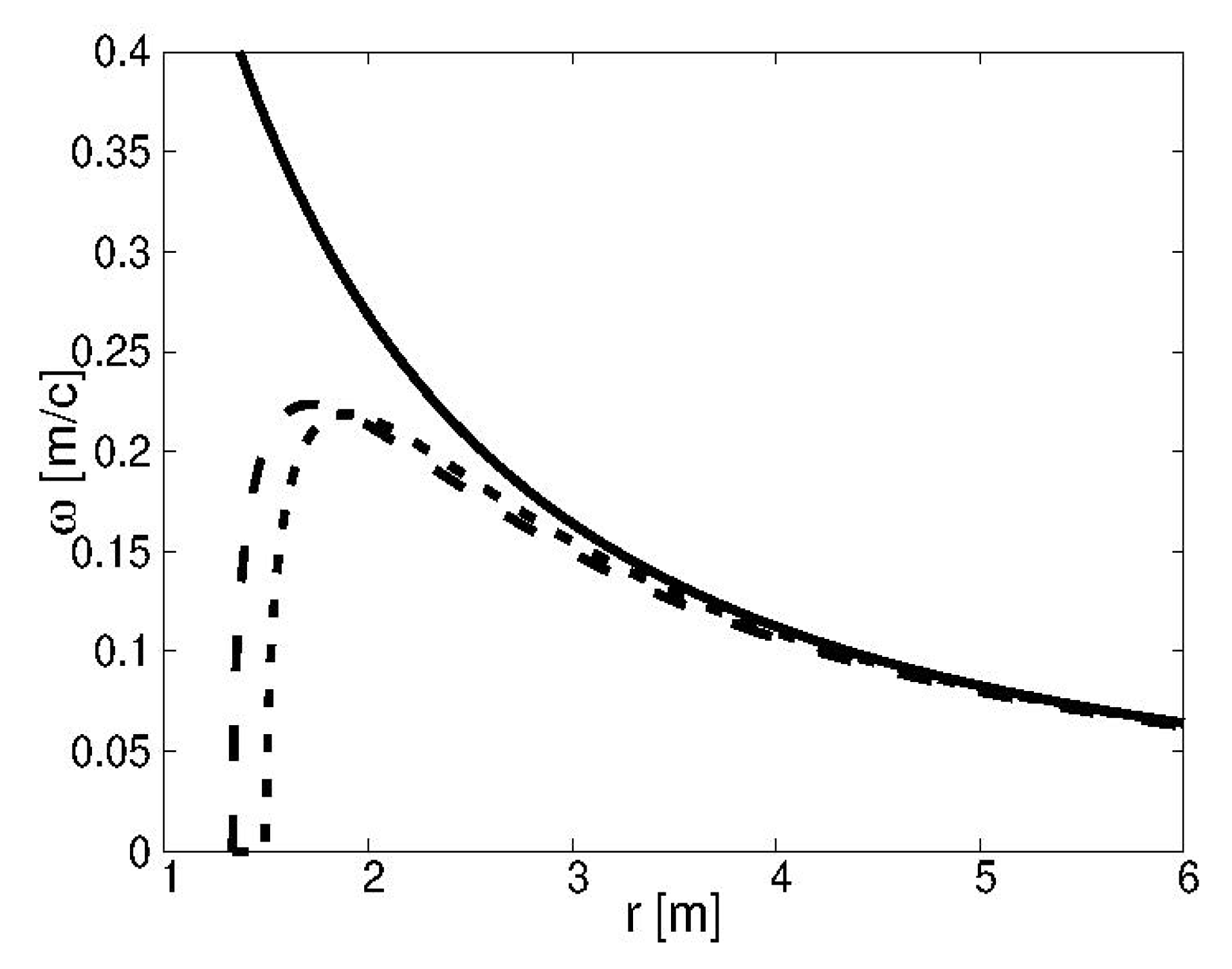
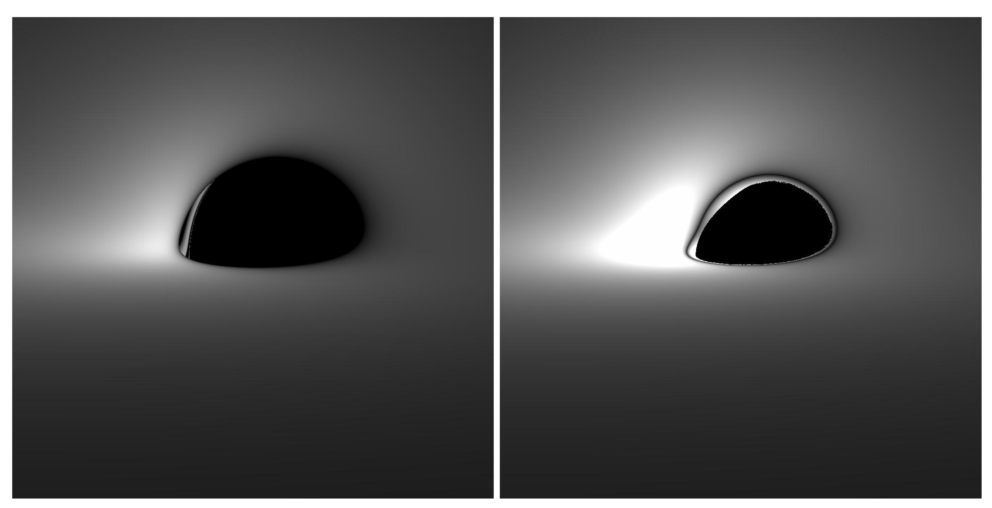
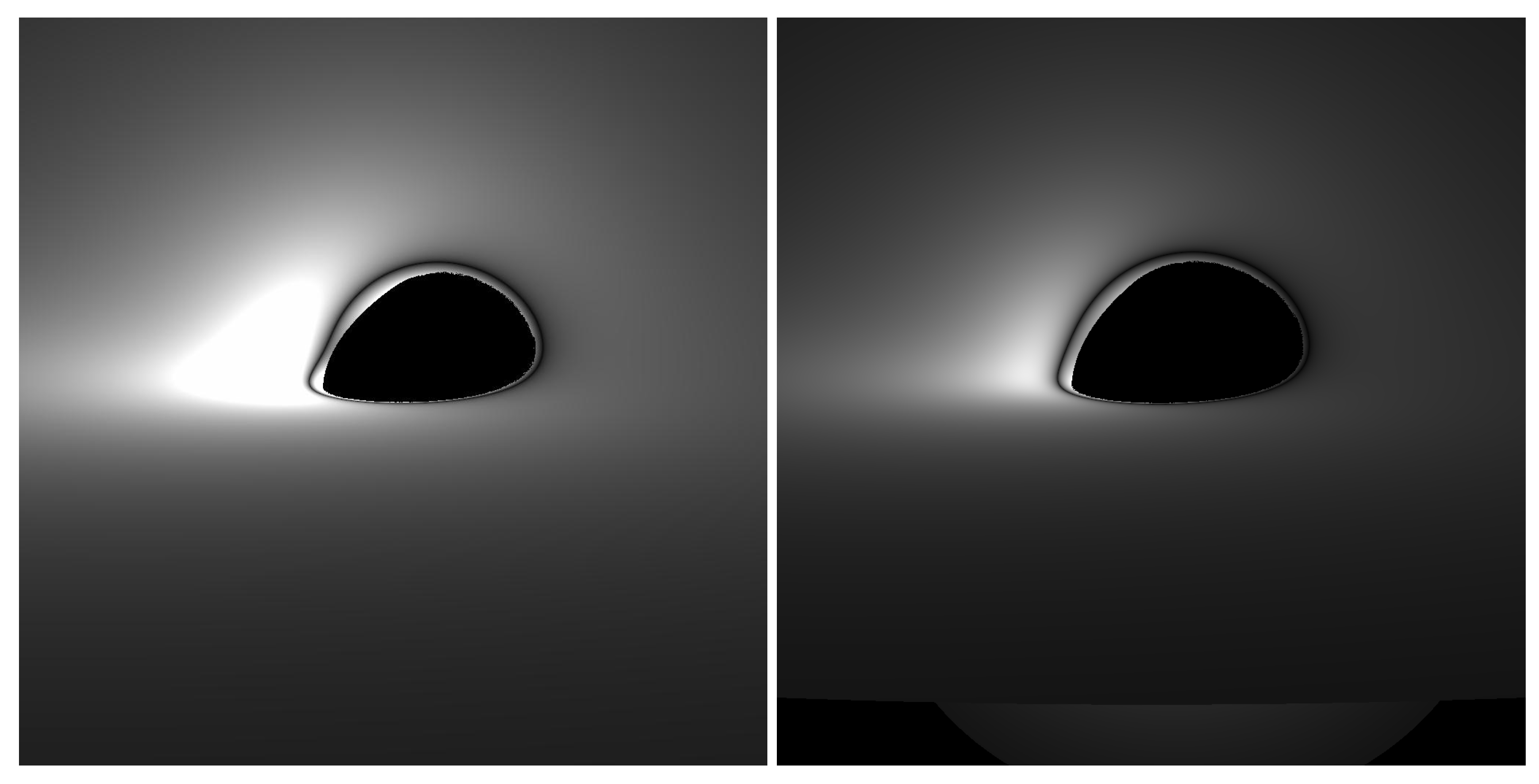
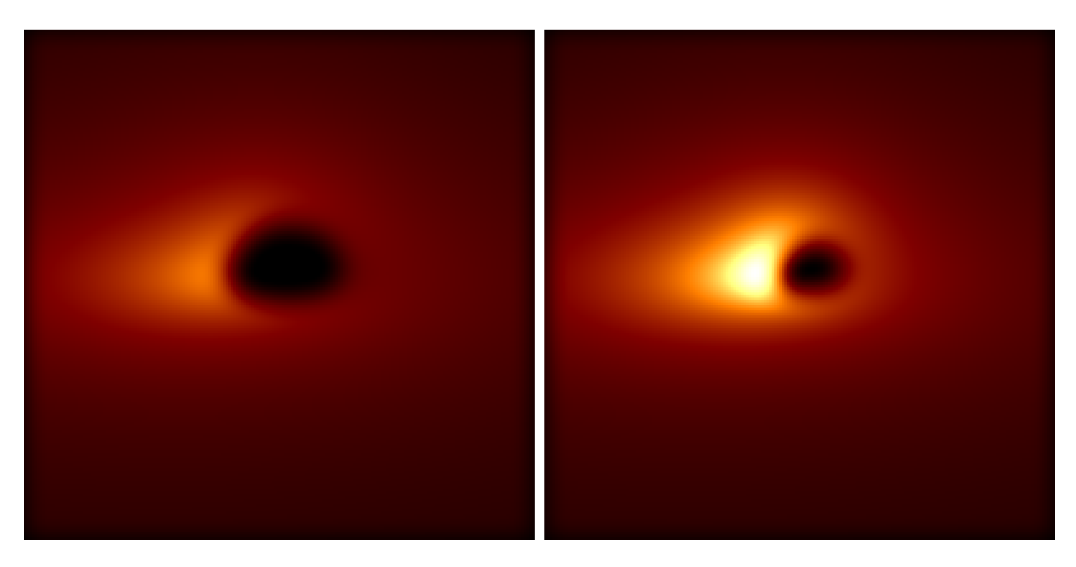
One of the most important predictions is that, when an accretion disc is present and for a rotation large enough, described by the parameter a, it shows a dark ring followed further in by a bright one. This is an effect of the dependence of a particle in a circular orbit, whose frequency shows a maximum and falls off for smaller r. At the maximum, neighboring orbitals have approximately the same orbital frequency, thus friction is low and no light emission is produced. Below and above the position of the maximum in the orbital frequency, it shows a change for neighboring orbital and friction is large, resulting in a stronger light emission. We also compared the GR simulation with the pc-GR one, taking into account the low resolution of 20 μ a s , similar to the EHT observation. From this we can conclude that there is, for now, little possibility to see any structural differences. Only an increase in the resolution by a factor of 5 can probably show differences between GR and pc-GR. Until such a resolution can be obtained, a couple of decades have to pass because it will imply to put radio-telescopes in the orbit of the moon and beyond. Nevertheless, the pc-GR can be tested with these telescopes in future. We are currently in contact with members of the EHT on how to obtain a Fourier transform from our pictures, which is what the EHT observes. We plan to look for details in the intensity distribution and its Fourier transform. Unfortunately, we cannot present any results on this yet.
This phenomenon of rings depends on the rotational parameter a: For low a, the last stable orbit follows the one of GR, only further in. The result is a similar pattern of light emission in pc-GR, but, at a higher value, because the last stable orbit reaches further in and, thus, more energy is released which is distributed within the disc. Note that, for a = 1 m 0 also in GR, no light ring can be observed because the inner edge of the accretion disk is at r = m 0 , while the light ring is at larger r. Thus, the light ring is hidden by the accretion disk.
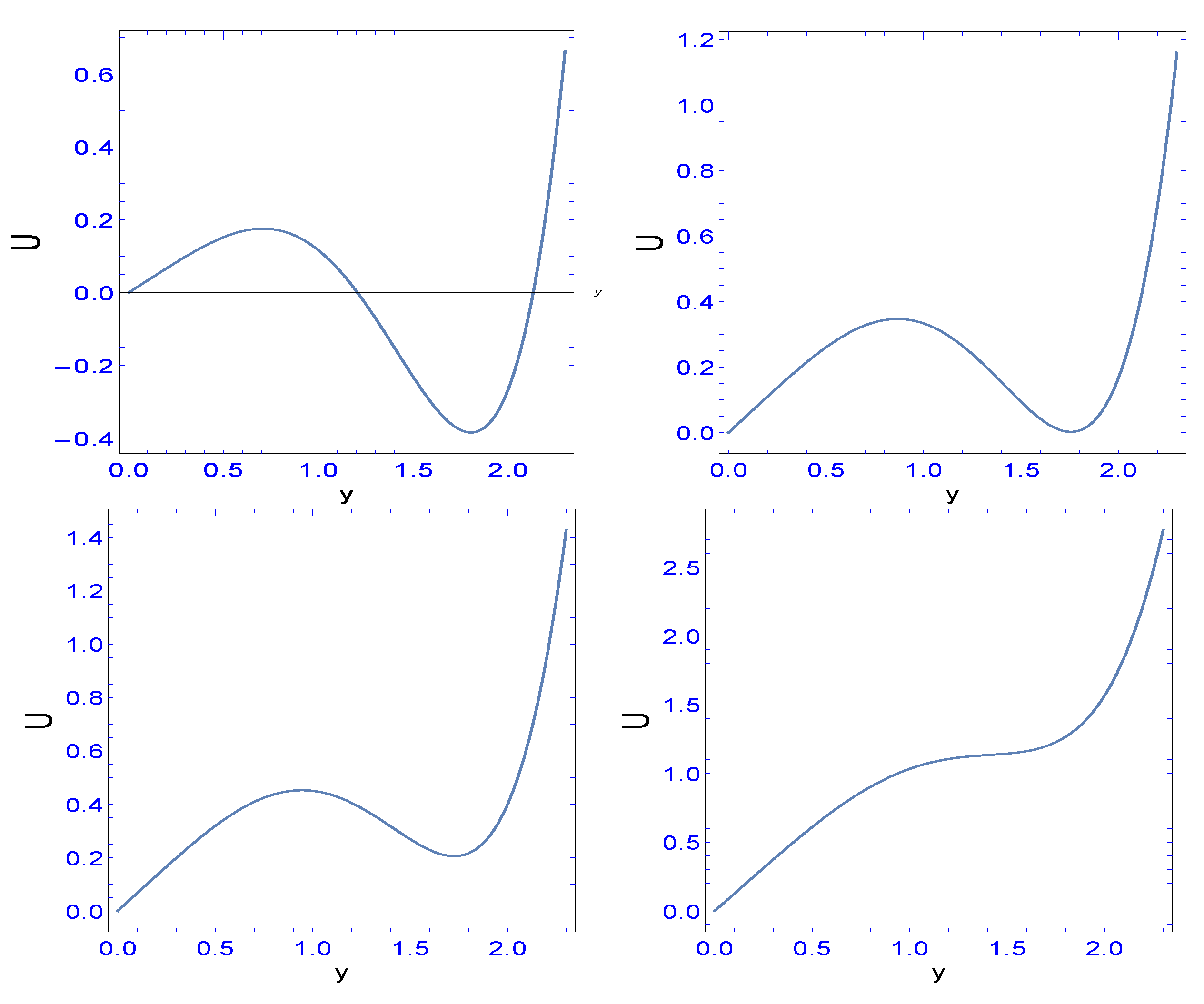
As a new contribution, we showed that the disappearance of the event horizon can be related to a phase transition, which is of the order of 3 when we reach the points where the surface of critical points has a singularity in its derivative. What consequences it may have is not clear to us and we are investigating it further.
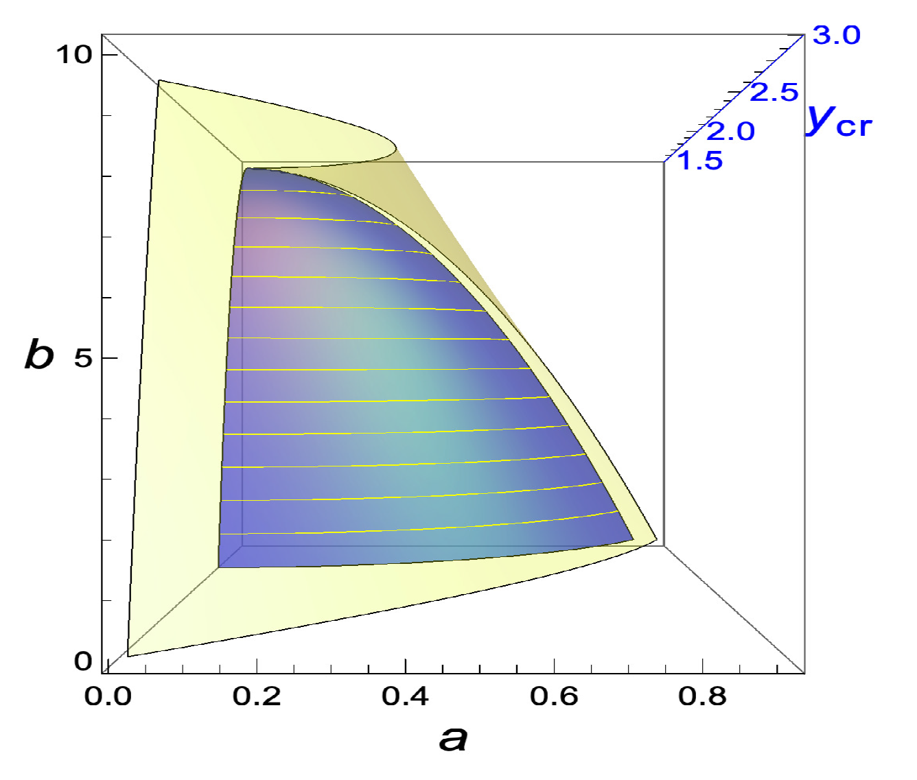
Finally, we discussed the light-ring in the orbital plane ( θ = π 2 ). We also found that, at the moment, some dark energy is accumulated around a black hole, and there is a region where the light-ring ceases to exist from a certain a-value on! The range increases with b n . We found that the critical surface of the light-ring engulfs the one of the event horizon.
Thus, adding even a small amount of dark energy around a large mass, leads for a certain a-value on to the disappearance of the event horizon and also eliminates the existence of a light-ring! One has to not assume a sufficient large value of b n in order for no event horizon or light-ring to exist, though the limiting value of b n = b n m a x serves that, for any a, no horizon exists.
Though a fluid identified with a dark energy is introduced, this fluid is treated classically, as all of the approaches presented in this review. We hope that the results may shed some light on how to include quantum mechanical effects directly. Often, classical treatments can shed some light on the quantum mechanical extension of the theory. The connection to a quantum mechanical description may be the reproduction of the dark energy behavior near a large mass, requiring first the observational confirmation of the structures predicted by the pc-GR.

Author Contributions

Both authors contributed jointly to all results presented in this publication.

Funding

This project was financed partially from the UNAM-PAPIIT under the project number IN100418.

Conflicts of Interest

The authors declare no conflict of interest.

References

  1. Will, C.M. The Confrontation between General Relativity and Experiment. Living Rev. Relativ. 2006, 9, 3. [Google Scholar] [CrossRef] [PubMed]
  2. Abbott, B.P.; Abbott, R.; Abbott, T.D.; Abernathy, M.R.; Acernese, F.; Ackley, K.; Adams, C.; Adams, T.; Addesso, P.; Adhikari, R.X.; et al. Observation of gravitational waves from a binary black hole merger. Phys. Rev. Lett. 2016, 116, 061102. [Google Scholar] [CrossRef] [PubMed]
  3. Akiyama, K.; et al. [The Event Horizon Telescope Collaboration]. First M87 Event Horizon Telescope Results. I. The shadow of the supermassive black hole. Astrophys. J. 2019, 875, L1. [Google Scholar]
  4. Akiyama, K.; et al. [The Event Horizon Telescope Collaboration]. First M87 Event Horizon Telescope Results. II. Array and Instrumentation. Astrophys. J. 2019, 875, L2. [Google Scholar]
  5. Akiyama, K.; et al. [The Event Horizon Telescope Collaboration]. First M87 Event Horizon Telescope Results. III. Data Processing and Calibration. Astrophys. J. 2019, 875, L3. [Google Scholar]
  6. Akiyama, K.; et al. [The Event Horizon Telescope Collaboration]. First M87 Event Horizon Telescope results. IV. Imaging the Central Supermassive Black Hole. Astrophys. J. 2019, 875, L4. [Google Scholar]
  7. Akiyama, K.; et al. [The Event Horizon Telescope Collaboration]. First M87 Event Horizon Telescope results. V. Physical origin of the asymmetric ring. Astrophys. J. 2019, 875, L5. [Google Scholar]
  8. Akiyama, K.; et al. [The Event Horizon Telescope Collaboration]. First M87 Event Horizon Telescope Results. VI. The Shadow and Mass of the Central Black Hole. Astrophys. J. 2019, 875, L6. [Google Scholar]
  9. Hess, P.O.; Schäfer, M.; Greiner, W. Pseudo-Complex General Relativity; Springer: Heidelberg, Germany, 2015. [Google Scholar]
  10. Schäfer, M.; Hess, P.O.; Greiner, W. Geometry of pseudo-complex General Relativity. Astron. Nachr. 2014, 335, 751–756. [Google Scholar] [CrossRef]
  11. Hess, P.O.; Greiner, W. Pseudo-complex general relativity. Int. J. Mod. Phys. E 2009, 18, 51–77. [Google Scholar] [CrossRef]
  12. Schönenbach, T.; Caspar, G.; Hess, P.O.; Boller, T.; Müller, A.; Schäfer, M.; Greiner, W. Experimental tests of pseudo-complex General Relativity. Mon. Not. R. Astron. Soc. 2013, 430, 2999. [Google Scholar] [CrossRef]
  13. Hess, P.O. Review on the Pseudocomplex General Relativity and Dark Energy. Adv. High Energy Phys. 2019, 2019, 1840360. [Google Scholar] [CrossRef]
  14. Schönenbach, T.; Caspar, G.; Hess, P.O.; Boller, T.; Müller, A.; Greiner, W. Ray-tracing in pseudo-complex General Relativity. Mon. Not. R. Astron. Soc. 2014, 442, 121–130. [Google Scholar] [CrossRef] [Green Version]
  15. Hess, P.O.; Algalán, M.; Schönenbach, T.; Greiner, W. Simulations of accretion disks in pseudo-complex General Relativity. Astron. Nachr. 2015, 336, 722. [Google Scholar] [CrossRef]
  16. Boller, T.; Hess, P.O.; Müller, A.; Stöcker, H. Predictions of the pseudo-complex theory of gravity for EHT observations: I. Observational tests. Mon. Not. R. Astron. Soc. Lett. 2019, 485, L34. [Google Scholar] [CrossRef]
  17. Hess, O.; Boller, T.; Müller, A.; Stöcker, H. Predictions of the pseudo-complex theory of Gravity for EHT observations – II: Theory and predictions. Mon. Not. R. Astron. Soc. Lett. 2019, 485, L121–L125. [Google Scholar] [CrossRef]
  18. Rodríguez, I.; Hess, P.O.; Schramm, S.; Greiner, W. Neutron stars within pseudo-complex general relativity. J. Phys. G 2014, 41, 105201. [Google Scholar] [CrossRef]
  19. Caspar, G.; Rodríguez, I.; Hess, P.O.; Greiner, W. Vacuum fluctuation inside a star and their consequences for neutron stars, a simple model. Int. J. Mod. Phys. E 2016, 25, 1650027. [Google Scholar] [CrossRef] [Green Version]
  20. Rodríguez, I.; Hess, P.O.; Schramm, S.; Greiner, W. Baryonic properties of neutron stars within pseudo-complex General Relativity. Astron. Nachr. 2010, 335, 745. [Google Scholar] [CrossRef]
  21. Hess, P.O.; Maghlaoui, L.; Greiner, W. The Robertson–Walker metric in a pseudo-complex general relativity. Int. J. Mod. Phys. E 2010, 19, 1315–1339. [Google Scholar] [CrossRef]
  22. Hess, P.O.; Maghlaoui, L.; Greiner, W. There are No Black Holes—Pseudo-Complex General Relativity: Review and Some Predictions. Int. J. Mod. Phys D 2010, 19, 1217–1232. [Google Scholar] [CrossRef]
  23. Lundgren, A.P.; Bondarescu, M.; Bondarescu, R. Depressing de Sitter in the Frozen Future. arXiv 2012, arXiv:1201.1298. [Google Scholar]
  24. Bondarescu, R.; Lundgren, A.P.; Bondarescu, M. The Physics of the Far Future. arXiv 2013, arXiv:1305.6838. [Google Scholar]
  25. Hess, P.O. The black hole merger event GW150914 within a modified theory of general relativity. Mon. Not. R. Astron. Soc. 2016, 462, 3026. [Google Scholar] [CrossRef]
  26. Hess, P.O.; López-Moreno, E. Regge-Wheeler and Zerilli equations within a modified theory of general relativity. Astron. Nachr. 2019, 340, 89–94. [Google Scholar] [CrossRef] [Green Version]
  27. Nielsen, A.B.; Birnholz, O. Testing pseudo-complex general relativity with gravitational waves. Astron. Nachr. 2018, 339, 298–305. [Google Scholar] [CrossRef]
  28. Nielsen, A.B.; Birnholz, O. Gravitational wave bounds on dirty black holes. Astron. Nachr. 2019, 340, 116–120. [Google Scholar] [CrossRef] [Green Version]
  29. Gilmore, R. Catastrophe Theory for Scientists and Engineers; Wiley: New York, NY, USA, 1981. [Google Scholar]
  30. Einstein, A. A generalization of the relativistic theory of gravitation. Ann. Math. 1945, 46, 578. [Google Scholar] [CrossRef]
  31. Einstein, A. A generalized theory of gravitation. Rev. Mod. Phys. 1948, 20, 35–39. [Google Scholar] [CrossRef]
  32. Born, M. A Suggestion for Unifying Quantum Theory and Relativity. Proc. Roy. Soc. A 1938, 16, 291. [Google Scholar] [CrossRef]
  33. Born, M. Reciprocity Theory of Elementary Particles. Rev. Mod. Phys. 1949, 21, 463. [Google Scholar] [CrossRef]
  34. Caianiello, E.R. Is there a maximal acceleration? Nuovo Cim. Lett. 1981, 32, 65–70. [Google Scholar] [CrossRef]
  35. Kelly, P.F.; Mann, R.B. Ghost properties of algebraically extended theories of gravitation. Class. Quantum Gravity 1986, 3, 705. [Google Scholar] [CrossRef]
  36. Hess, P.O.; Greiner, W. Centennial of General Relativity: A Celebration; Vasconcellos, C.A.Z., Ed.; World Scientific: Singapore, 2017; p. 97. [Google Scholar]
  37. Birrel, N.D.L.; Davies, P.C.W. Quantum Field in Curved Space; Cambridge University Press: Cambridge, UK, 1986. [Google Scholar]
  38. Visser, M. Gravitational vacuum polarization. II. Energy conditions in the Boulware vacuum. Phys. Rev. D 1996, 54, 5116. [Google Scholar] [CrossRef] [PubMed]
  39. Volkme, G.L.R. Um Objeto Compacto Excotico na Relatividade Geral Pseudo-Complexa. Ph.D. Thesis, Federal University of Rio Grande do Sul, Porto Alegre, Brazil, March 2018. [Google Scholar]
  40. Razeira, M.; Hadjimichef, D.; Machado, M.T.V.; Köpp, F.; Volkmer, G.L.; Vasconcellos, C.A.Z. Effective field theory for neutron stars with WIMPS in the pc-GR formalism. Astron. Nachr. 2017, 338, 1073. [Google Scholar] [CrossRef]
  41. Hadjimichef, D.; Volkmer, G.L.; Gomes, R.O.; Vasconcellos, C.A.Z. Memorial Volume: Walter Greiner; Hess, P.O., Stöcker, H., Eds.; World Scientific: Singapore, 2018. [Google Scholar]
  42. Volkmer, G.L.; Hadjimichef, D. Mimetic dark matter in pseudo-complex General Relativity. Int. J. Mod. Phys. Conf. Ser. 2017, 45, 1760012. [Google Scholar] [CrossRef]
  43. Volkmer, G.L.; Razeira, M.; Hadjimichef, D.; Köpp, F.; Vasconcellos, C.A.Z.; Bodmann, B. Pseudo-complex general relativity and the slow rotation approximation for neutron stars. Astron. Nachr. 2019, 340, 205–208. [Google Scholar] [CrossRef] [Green Version]
  44. MATHEMATICA 11.3.0.0; Wolfram Research Foundation: Champaign, IL, USA, 2018.
  45. Available online: https://github.com/peterottohess/phase-transitions (accessed on 27 August 2019).
  46. Caspar, G.; Schönenbach, T.; Hess, P.O.; Schäfer, M.; Greiner, W. Pseudo-complex general relativity: Schwarzschild, Reissner–Nordström and Kerr solutions. Int. J. Mod. Phys. E 2012, 21, 1250015. [Google Scholar] [CrossRef]
  47. Balakrishna, J.; Bondarescu, R.; Moran, C.C. Self-gravitating stellar collapse: Explicit geodesics and path integration. Front. Astron. Space Sci. 2016, 3, 29. [Google Scholar] [CrossRef]
  48. Vincent, F.H.; Paumard, T.; Gourgoulhon, E.; Perrin, G. GYOTO: A new general relativistic ray-tracing code. Class. Quantum Gravity 2011, 28, 225011. [Google Scholar] [CrossRef]
  49. Page, D.N.; Thorne, K.S. Disk-accretion onto a black hole. Time-averaged structure of accretion disk. Astrophys. J. 1974, 191, 499–506. [Google Scholar] [CrossRef]
  50. Hess, P.O.; Boller, T.; López-Moreno, E. Comparison of the predictions of the pc-GR to the observations of the EHT. Astron. Nachr. 2019, in press. [Google Scholar]
  51. Adler, R.; Bazin, M.; Schiffer, M. Introduction to General Relativity; McGraw-Hill: New York, NY, USA, 1975. [Google Scholar]
  52. Baranov, A.M. The catastrophe theory, Petrov’s algebraic classification and gravitational phase transitions. Grav. Cosm. 2011, 17, 170. [Google Scholar] [CrossRef]
  53. López-Moreno, E.; Grether, M.; Velázquez, V.J. Energy level structure and quantum phase transitions of spin systems with nonaxially symmetric Hamiltonians. Phys. A 2011, 44, 475301. [Google Scholar] [CrossRef]
  54. Berry, M.V. Waves and Thom’s theorem. Adv. Phys. 1976, 25, 1–26. [Google Scholar] [CrossRef]
  55. Giddings, S.B.; Psaltis, D. Event horizon telescope observations as probes for quantum structure of astrophysical black holes. arXiv 2018, arXiv:1606.07814. [Google Scholar] [CrossRef]
Figure 1. The dependence of the orbital frequency of a particle in a circular orbit on the radial distance. The upper curve shows the result for GR and the lower two curves for pc-GR. The one with its maximum further to the left corresponds to n = 3 and the other one to n = 4 . Equation (21) was used with b = 64 27 for n = 3 and b = 81 8 for n = 4 .
Universe 05 00191 g001
Figure 2. The position of the Innermost Stable Circular Orbit (ISCO) for n = 3 ( left panel) and n = 4 (right panel) is plotted versus the rotational parameter a. The upper curve in each figure corresponds to GR and the lower curve to pc-GR. In the region to the left of the pc-GR curve, the orbits are unstable in pc-GR; above and to the right, the orbits are stable. For small values of a, the ISCO in pc-GR follows more or less the one of GR, but at smaller values of r. From a certain value of a on, stable orbits are allowed until the surface of the star. For n = 3 , this limit is approximately a = 0.4 m 0 and, for n = 4 , it is above a = 0.5 m 0 . For larger values of a, all orbits are stable in pc-GR. For the construction of the curve for n = 3 , Equation (42) of [12] was used. This equation has to be modified for n = 4 , which is direct. It can be retrieved from [45], where all the routines used here are openly accessible.
Universe 05 00191 g002
Figure 3. Infinite, counter clockwise rotating geometrically thin accretion disc around a rotating compact object, viewed from an inclination of 80 . The disc model by [49] was used. The right panel is a simulation within pc-GR for a = 0 and the right panel for a = 0.9 m 0 . Both figures are for n = 3 . (Figures taken from [14,16,17].) The figures were obtained using the open accessible 2014 version of the GYOTO routines [48].
Universe 05 00191 g003
Figure 4. The explanation is the same as in Figure 3. The left panel shows the simulation for pc-GR and n = 3 (the same as the right panel in Figure 3), while the right panel is a simulation for n = 4 . As noted, the position of the dark and bright rings are shifted slightly to larger radial distances. The figures were obtained using the open accessible 2014 version of the GYOTO routines [48]. For n = 4 , the modified C++ rountines can be retrieved in [45].
Universe 05 00191 g004
Figure 5. Infinite, counterclockwise rotating geometrically thin accretion disc around static rotating compact objects viewed from an inclination of 70 . The upper row and the left panel show the result for a resolution of 0.5 μ a s while the right panel corresponds to a resolution of 20 μ a s . In the upper row, a = 0.6 m 0 . The lower figure is taken from the EHT results, rotated by 90 . The figures were obtained using the open accessible 2014 version of the GYOTO routines [48]. For n = 4 , the modified C++ routines can be retrieved in [45].
Universe 05 00191 g005
Figure 6. Simulations of accretion discs for an inclination of 60 and a = 0.6 m. A resolution of 20 μ a s was assumed [50]. The left panel shows the result for GR and the right one for pc-GR. As seen, the GR and pc-GR cannot be distinguished clearly. The dark center in GR is slightly larger than in pc-GR, which is also noted in the calculation of fluxes (see main text). The figures were obtained using the open accessible 2014 version of the GYOTO routines [48]. For n = 4 , the modified C++ rountines can be retrieved in [45].
Universe 05 00191 g006
Figure 7. The intensity distribution for pc-GR (upper) curve and GR (lower curve). The rotational parameter a is changed from 0.6 m 0 to 0.9 m 0 ( m = m 0 ) starting on the left in the upper row and ending to the right in the lower row, in steps of 0.1 m 0 . The intensity in pc-GR is always larger. The peak shifts to the left (lower distances) as a increases. For a = 0.9 m 0 , the peak is around r = 0.4 m 0 , while the peak of the pc-GR curve is always at lower r. The intensities are obtained using (23). The relation between L z and E can be retrieved from [14].
Universe 05 00191 g007
Figure 8. Shown is the surface of allowed horizons for n = 3 (left panel) and n = 4 (right panel); also shown is the projected curve of the separatrix (blue curve). The vertical axis denotes r in units of m 0 = m , the x-axis the a in units of m 0 and the y-axis the b n = b parameter. The figures are obtained using (25). The corresponding MATHEMATICA [44] tool can be retrieved from [45].
Universe 05 00191 g008
Figure 9. Shown are two sets for n = 4 ( a = 0 and a = 0.5 m 0 , respectively), of the position of the extrema as a function of b n . For each a, the upper curve corresponds to a maximum and the lower one to the position of the minimum. The two curves meet at a certain b n = b value, which increases with decreasing a. The dashed line corresponds to a = 0.5 m 0 , while the continuous line is for a = 0 . Equation (25) was used and the corresponding MATHEMATICA routine can be retrieved from [45].
Universe 05 00191 g009
Figure 10. Shown are four cuts of the potential at a = 0.5 m 0 and, respectively from upper left to lower right, for the values of ( n = 4 ) b n = 2, 3.3, 4 and 7.5. For b n = 2 , the deformed minimum is at negative values; for b n = 3.3 , it is at the same height as for U at y = 0 , for b = 4, the deformed minimum is at positive values and, at 7.5, it is disappearing, being close to the point where the maximum and minimum join, as shown in Figure 9. For the potential, (27) was used. The corresponding MATHEMATICA routine can be retrieved from [45].
Universe 05 00191 g010
Figure 11. The critical surfaces for the horizon (inner surface) and the light-ring (outer surface). The critical surface of the light-ring follows the one of the horizon, only further out. Note the region where the light-ring does not exist. The b value is equal to b n . For the construction of the light ring surface, (38) was used. The corresponding MATHEMATICA routine can can be retrieved from [13].
Universe 05 00191 g011

