Observing the Dark Sector ^†

Abstract

Despite the observational success of the standard model of cosmology, present-day observations do not tightly constrain the nature of dark matter and dark energy and modifications to the theory of general relativity. Here, we will discuss some of the ongoing and upcoming surveys that will revolutionize our understanding of the dark sector.

1. Introduction

The standard model of cosmology is of utter simplicity: assuming General Relativity and small perturbations about a spatially homogeneous and isotropic background model, it can easily account for basically all cosmological observations, probing a vast range of scales in space and time with just six parameters. According to the standard model of cosmology the universe is dominated by a mysterious matter called “dark matter” and a mysterious energy called “dark energy.” This conclusion is supported, for example, by observations of supernovae Ia (SNIa) [1,2], of the Baryonic Acoustic Oscillations (BAO) [3,4], of the anisotropies of the Cosmic Microwave Background (CMB) [5,6] and of the weak lensing of galaxies [7,8]. Dark matter seeded the formation of galaxies while dark energy is driving them apart by causing the universe to accelerate, a phenomenon that was conjectured in the early 1990s [9], observed in 1998 [10,11] and awarded the Nobel Prize in 2011.

However, a satisfactory theoretical explanation of dark matter and dark energy—the so-called dark sector—is still lacking and their properties are not yet well constrained by the data [12,13,14]. According to the standard model of cosmology, baryons—particles belonging to the successful standard model of particle physics—constitute only 5% of the energy content of the universe. The remaining 95% is left to the dark sector. Approximately 25% consists of a yet-undetected matter component, which is thought to be a massive particle of non-baryonic nature which interacts through gravity and weak interaction only. It is named “cold dark matter” because it neither emits nor absorbs light or other electromagnetic radiation (and so it is dark) and it moves slowly compared to the speed of light (and so it has a low temperature). Dark energy is responsible for the missing 70%. The best candidate to date is the “cosmological constant,” the energy of the vacuum and an arbitrary constant of nature in the general relativity. Its fundamental property—gravitational repulsion for positive energy density—causes the expansion of the universe to accelerate, as mentioned earlier.

Therefore, the standard model of cosmology is facing a formidable challenge as it is asked to account for not one but two unknown components. It is undeniable that cosmology itself is at the moment built on shaky foundations, relying on an unexplained dark sector for observations to fit the model. The implications of this cannot be overstated. This is the motivation for the large theoretical and experimental effort that is being deployed to better understand the nature of the dark sector.

Indeed, the scientific study of the universe is on the verge of a revolution. New cosmological galaxy surveys will map the universe in unprecedented detail over volumes which we have only been able to imagine in vast computer simulations. Gravitational-wave survey will soon produce massive catalogs of events able to probe the theory of General Relativity in the uncharted strong-field limit and determine the presently widely unknown stellar black hole mass function, besides providing a new handle to measure late cosmological acceleration. Finally, 21-cm survey will map the density of the universe at even larger scales, covering almost all the observable universe.

In the following we will summarize how these surveys will revolutionize our understanding of the dark sector, pinning down the phenomenology of dark matter and dark energy and so triggering major progress in our understanding of the fundamental interactions of nature.

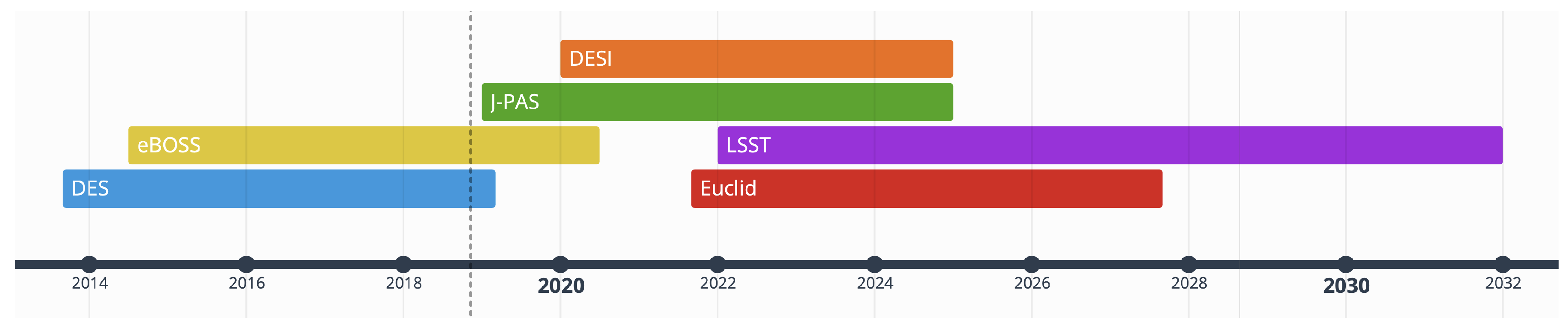
2. Galaxy Surveys

Figure 1 shows the timeline of the ongoing and upcoming galaxy surveys that will be discussed in this section. Surveys have been classified according to their constraining power on the dark energy equation of state [15]:

$$w=\frac{p}{\rho },$$

(1)

where p is the pressure of the fluid and $\rho$ its energy density. Dark energy has been constrained to have an equation of state of $w\approx -1$, while dark matter has been found compatible with $w\approx 0$, a pressureless (dust) fluid.1 If $w=-1$, one has the cosmological constant and the Lambda Cold Dark Matter ($\mathsf{\Lambda }$CDM) model. If one lets w free, then one has the wCDM model.

The constraining power on the dark energy equation of state is quantified via the so-called Figure of Merit (FoM), which is defined as

$$\mathrm{FoM}={det}^{-1}F(w_0,w_a),$$

(2)

where F is the (marginalized) Fisher matrix relative to the dark energy equation of state, parameterized according to2

$$w\left(a\right)=w_0+(1-a)w_a.$$

(3)

Stage-II experiments (previous to DES) feature a FoM less than 50, Stage-III experiments about 50–200 and Stage-IV experiments about 200+. DES and eBOSS are Stage-III level, J-PAS approches Stage IV and the remaining are all “Stage IV.”

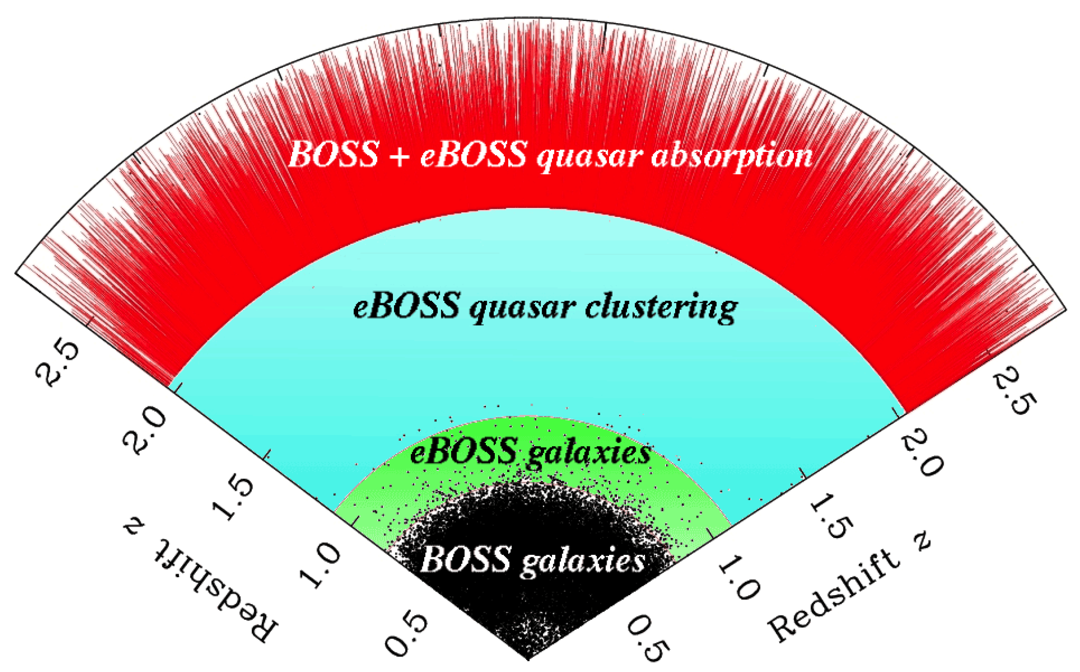
2.1. Extended Baryon Oscillation Spectroscopic Survey

The Extended Baryon Oscillation Spectroscopic Survey (eBOSS) is part of the fourth phase of the Sloan Digital Sky Survey (SDSS-IV) and extends the Baryon Oscillation Spectroscopic Survey (BOSS, part of SDSS-III) to much higher redshifts. The eBOSS survey started on July 2014 and will last 6 years and will produce the largest volume survey to date, see Figure 2. eBOSS targets the observation of galaxies and quasars in a range of redshifts currently left uncharted by other maps of the large-scale structure of the universe.

300,000 luminous red galaxies (LRG) will be observed over 7500 deg${}^2$ in the redshift range $0.6<z<0.8$, 189,000 emission line galaxies (ELG) over 1000 deg${}^2$ in the range $0.6<z<1.0$ and 573,000 quasars over 7500 deg${}^2$ in the range $0.9<z<3.5$. This large catalog will produce 1–2% distance measurements from baryon acoustic oscillations in the redshift range $0.6<z<2.5$. At this time, the Data Release 14 (DR14) of the first 2 years of observations has been publicly released, see Reference [18] for the first measurement of baryon acoustic oscillations between redshift 0.8 and 2.2. See Reference [19] for further information.

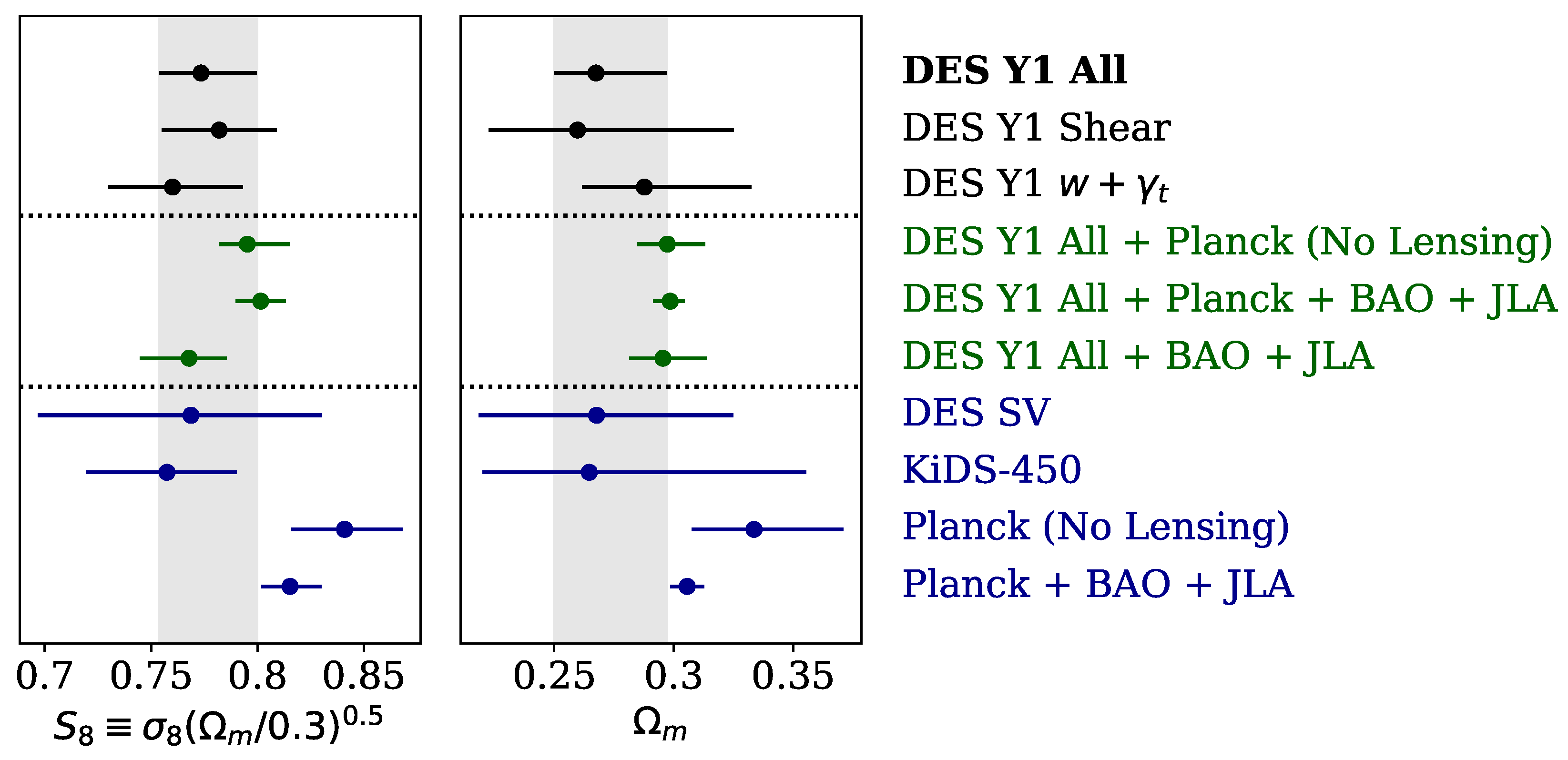
2.2. Dark Energy Survey

The Dark Energy Survey (DES)3 is a project that is mapping 5000 deg${}^2$ of the sky (approximately 1/8 of the whole sky) using 525 nights of observations in 5 years at the Blanco Telescope in the Cerro Tololo Inter-American Observatory in Chile. The project is led by Fermilab, a US national laboratory near Chicago and its current (third) Director is Rich Kron from the University of Chicago. There are more than 400 scientists from over 25 institutions in the US, Brazil, Spain, UK, Germany, Switzerland and Australia working on the project.

A large digital camera with 570 Megapixels in 62 CCD’s was built by the collaboration and installed in the telescope. This so-called DECam takes exposures using 5 filters (grizY) that provide an estimate of the photometric redshift of approximately 300 million objects. This large amount of data is transferred and processed at the National Center of Supercomputing Applications (NCSA) in Urbana-Champaign to generate a value-added catalogue.

The first light of DES was in 2012. There was a 6-month extension to the observation period that ends in January 2019. There are already more than 200 papers from the DES collaboration in the Inspire database. Results from the first year of observations have been published leading to several ground-breaking results, some of which will be mentioned below. Some highlights are:

• Produced the largest contiguous mass map of the Universe;
• Discovered nearly a score of Milky Way dwarf satellites and other Milky Way structures;
• Measured weak lensing cosmic shear, galaxy clustering and cross-correlations with CMB lensing and with clusters detected via X-ray and the Sunyaev-Zeldovich effect;
• Measured light curves for large numbers of type Ia supernovae and discovered a number of super-luminous supernovae (SLSN) including the highest-redshift SLSN so far;
• Discovered a number of redshift $z>6$ quasars (also known as QSOs or quasi-stellar objects);
• Discovered a number of strongly lensed galaxies and QSOs;
• Discovered a number of interesting objects in the outer Solar System;
• Found optical counterparts of GW events

DES combines four different observational probes in order to find the best constraints on dark energy:

• Distribution of 300 million galaxies, including measurements of the Baryon Acoustic Oscillation;
• Weak gravitational lensing of galaxies;
• Supernovae of type Ia;
• Counts of clusters of galaxies.

The main cosmological result of the first year of observations was published in Reference [7], a key paper which uses the results of other 11 papers. It combines measurements of three 2-point correlation functions involving galaxy positions and weak lensing (shear): galaxy-galaxy (galaxy clustering), galaxy-shear and shear-shear. Two galaxy samples are used:

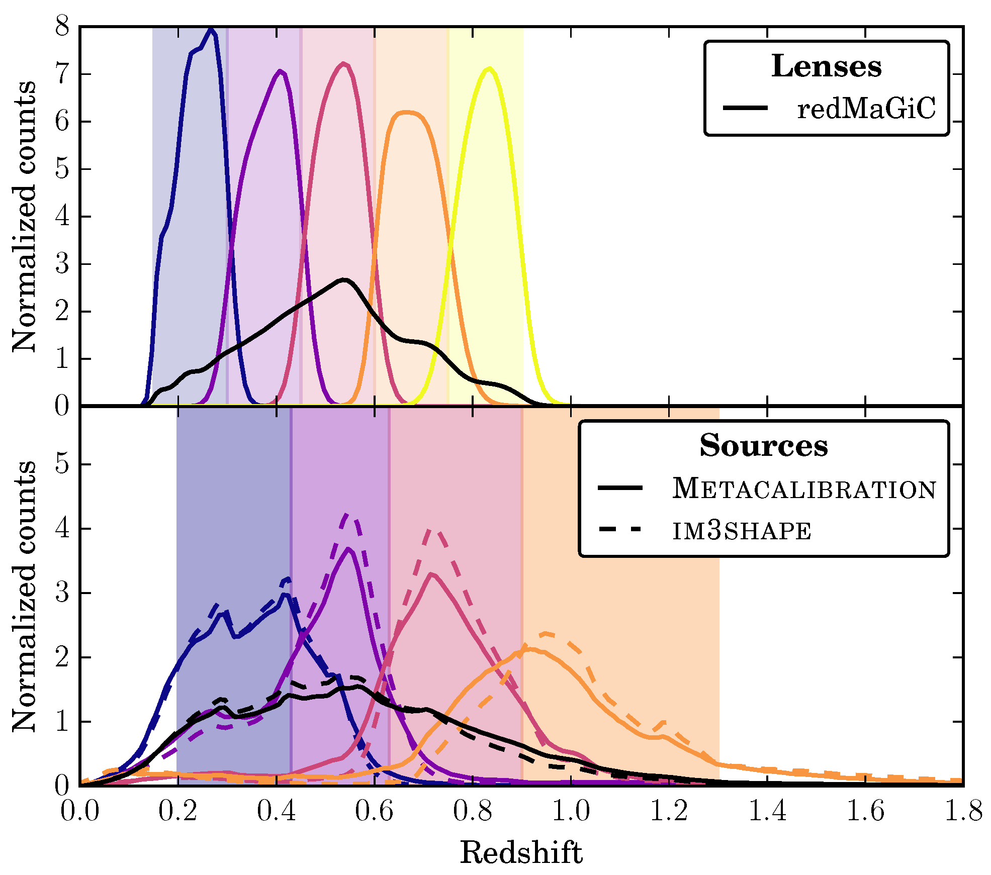
• “Shape catalogue”: 26M galaxies for cosmic shear measurements (source galaxies) divided into 4 redshift bins;
• “Position catalogue”: 650,000 luminous red galaxies (lens galaxies) for clustering measurements divided into 5 redshift bins.

The photometric redshift distributions for the two samples are shown in Figure 3.

The data vectors were defined using scale cuts to mitigate non-linear bias effects and it comprises 457 entries (different redshift bins, angular bins, correlation functions). We used a theoretical (halo-model based) covariance matrix (dimension 457 × 457) computed with the CosmoLike code validated with 800 lognormal mocks. For the Markov Chain Monte Carlos (MCMC) analysis we had 20 nuisance parameters (related to the redshift uncertainty, galaxy bias, intrinsic alignment and shear calibration) in addition to the usual 6 cosmological parameters for the spatially flat $\mathsf{\Lambda }$CDM model (7 for wCDM, where w is defined in Equation (1)). We concentrate the analysis on the two most sensitive parameters: ${\mathsf{\Omega }}_m$ and $S_8={\sigma }_8{({\mathsf{\Omega }}_m/0.3)}^{0.5}$, where ${\mathsf{\Omega }}_m$ is the matter density parameter and ${\sigma }_8$ is the root mean square mass fluctuation on a scale of $8h^{-1}$ Mpc. The matter density parameter is defined according to ${\mathsf{\Omega }}_m={\rho }_{m0}/{\rho }_{c0}$, where ${\rho }_{m0}$ is the present-day matter density and the present-day critical density is given by ${\rho }_{c0}=3H_0^2/\left(8\pi G\right)$, where $H_0$ is the Hubble-Lemaître constant and G is Newton’s gravitational constant. We also compare results from DES alone with DES combined with data such as CMB, BAO and SNIa, see Figure 4.

In Figure 5 we show the 1- and 2-$\sigma$ contours for the parameters $S_8$ and ${\mathsf{\Omega }}_m$ obtained from DES, Planck and combined. It’s amazing to see that, for the first time, results from large surveys of galaxies provide bounds on cosmological parameters that are competitive with the ones obtained from CMB. It also shows the consistency of the $\mathsf{\Lambda }$CDM model from the time of recombination where the CMB was generated to late times after galaxy formation.

DES data were analyzed also in the context of the wCDM model which features a constant equation of state w, see Figure 6. The result for w, when DES is combined with other data, provides the state-of-the-art determination of w [7]:

$$w=-{1.00}_{-0.04}^{+0.05},$$

(4)

in perfect agreement with $\mathsf{\Lambda }$CDM.

Other extensions of the $\mathsf{\Lambda }$CDM model were studied in Abbott et al. [20]:

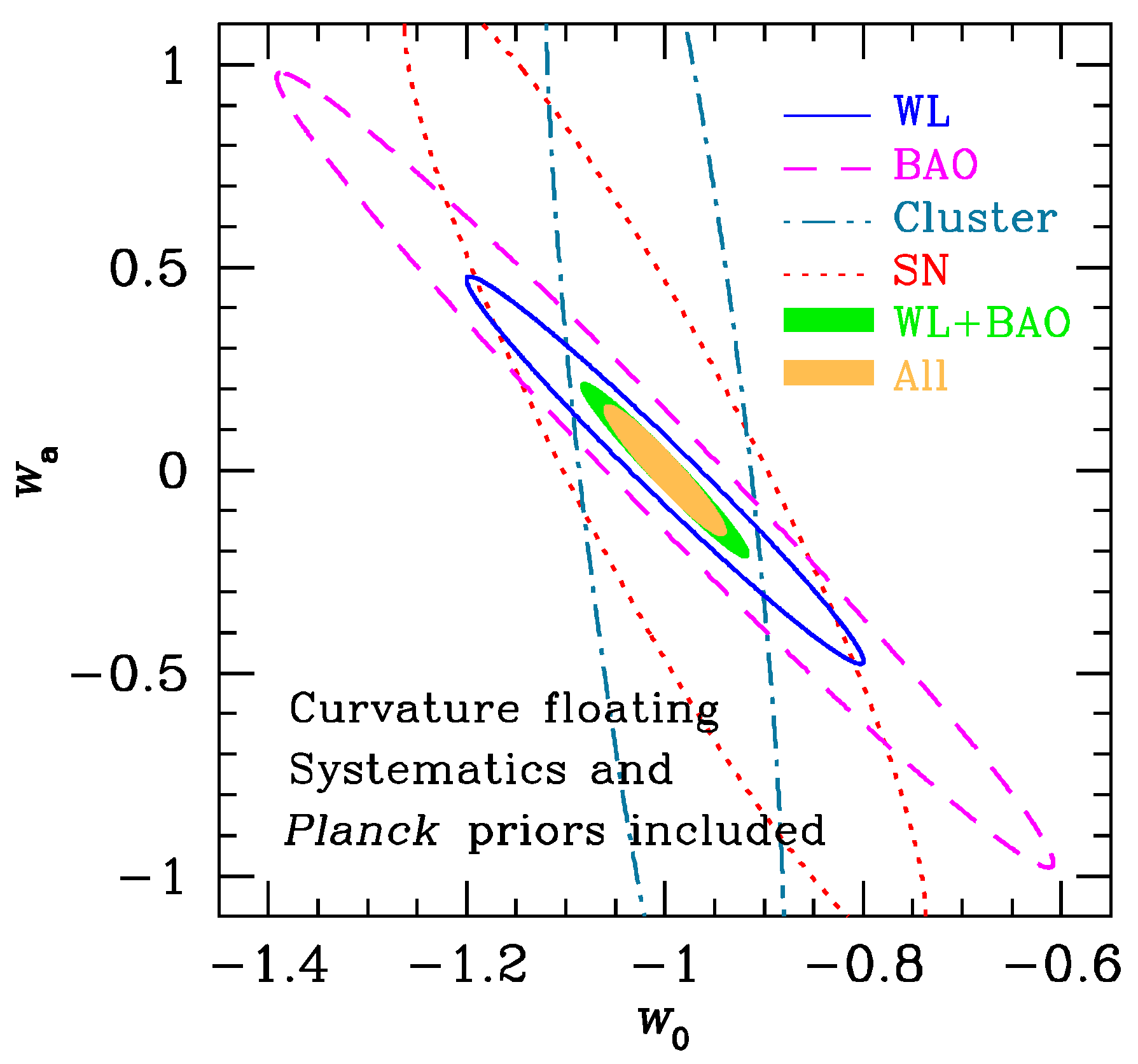
• Spatial curvature;
• The effective number of neutrinos species;
• Time-varying equation of state of dark energy, see Equation (1);
• Tests of gravity.

As an example, in Figure 7 we show the contour plots for $w_0$ and $w_a$ for DES and other external data. We can see that DES data from the first year of observation is still not competitive with other data.

The DES data also produced the measurement of what is called the shift parameter $\alpha$ which gives the location of the BAO peak with respect to a reference cosmology [21]. In Figure 8 we show the DES measurement of the angular diameter distance $D_A$, corresponding to the BAO feature, compared to other measurements at different redshifts.

2.3. Javalambre Physics of the Accelerating Universe Astrophysical Survey

The Javalambre Physics of the Accelerating Universe Astrophysical Survey (J-PAS—[22]) is a ground-based survey that is expected to begin scientific observations at the beginning of 2019. It features a dedicated 2.5 m telescope with an excellent étendue which sports a 1.2 Gigapixel camera with a very large field of view of $4.7{\mathrm{deg}}^2$. The observatory is in the mountain range “Sierra de Javalambre” (Spain), at an altitude of 2000 m, an especially dark region with the very good median seeing of ${0.7}^{″}$.

J-PAS will observe approximately $8500{\mathrm{deg}}^2$ of the sky via the revolutionary technique of quasi-spectroscopy: by observing with 54 narrow-band filters, two medium-band filters and three broad-band filters it will produce a pseudo-spectrum ($R\sim 50$) for every pixel, see Figure 9. Therefore, J-PAS really sits between photometric surveys such as DES and spectroscopic surveys such as DESI, fruitfully combining the advantages of the former (speed and low cost) with the ones of the latter (spectra). In particular, it will be possible to determine the redshift of galaxies with a precision of $0.003(1+z)$. In other words, it will be possible to accurately study the large scale structure of the universe using the galaxy and quasar catalogs produced by J-PAS. This makes J-PAS the first survey to approach the “Stage IV” level.

As far as the dark sector and modified gravity, the most interesting observables will be galaxy clustering and galaxy cluster number counts. Regarding the former, thanks to the very precise photo-z determinations and the large volume that will be explored, it will be possible to obtain excellent measurements of Baryonic Acoustic Oscillations (BAO) and Redshift Space Distortions (RSD) in a wide redshift range ($0<z<3$).

About 90 million luminous red galaxies (LRG) and emission line galaxies (ELG) (up to $z\sim 1.2$) and 2 million quasars (up to $z\sim 3$) are expected to be detected. Figure 10 and Figure 11 show the corresponding forecasts. See also References [24,25] where constraints using the multi-tracer method are discussed.

Regarding cluster counts, thanks again to its quasi-spectroscopic photometric redshift, J-PAS will be able to separate cluster members from foreground and background galaxies with very high accuracy. Indeed, the accuracy of the photometric redshift matches the typical velocity dispersion of massive clusters: this ability together with the large area covered will allow J-PAS to detect clusters to much lower masses and higher redshifts than conventional photometric wide-field surveys. J-PAS will produce a catalog of about 700 thousand clusters with more than 10 members, down to $\sim 3·{10}^{13}{M}_{\odot }$. See Figure 12 for a forecast. Weak lensing observations will also be carried out and will be used to calibrate the cluster mass determination.

Weak and strong gravitational lensing data will also contain important cosmological information. J-PAS will be a revolutionary observatory also regarding the study of supernovas, galaxy evolution and stellar physics. See Reference [22] for the full potential of the J-PAS survey.

2.4. Dark Energy Spectroscopic Instrument

The Dark Energy Spectroscopic Instrument (DESI) is a Stage IV ground-based dark energy experiment that will study, via a wide-area galaxy and quasar redshift survey, both the expansion history of the universe through baryon acoustic oscillations and the growth of structure through redshift-space distortions. DESI will be the successor to the BOSS survey and will complement imaging surveys such as DES and LSST. DESI will strongly constrain the nature of dark energy, theories of modified gravity and inflation and will provide tight limits on the sum of neutrino masses.

DESI will obtain optical spectra for tens of millions of galaxies and quasars, constructing a revolutionary 3D map spanning the nearby universe to 11 billion light years. This feat will be achieved using 5000 pencil-size robots that will position the optical fibers that will catch the light from distant objects and transmit it to the spectrographs. The DESI Survey will be conducted on the Mayall 4-m telescope at Kitt Peak National Observatory in Arizona (USA), starting at the beginning of 2020. See Figure 10 and Figure 11 for forecasts on radial and angular BAO and on the growth of structures. See Reference [27] for further information.

2.5. Euclid Consortium

The Euclid spacecraft [28] is currently under construction and scheduled for launch in the second half of 2021. During its mission, which will last at least 6 years, Euclid will observe approximately ${\mathsf{\Omega }}_{\mathrm{sky}}=\mathrm{15,000}{\mathrm{deg}}^2$ of the extra-galactic sky, which is about half of the total sky facing away from the Milky Way.

Euclid is the combination of two complementary probes. The 1.2-m Korsch telescope will feed, via a beam splitter, the visible band imager (VIS) and the near infrared spectrometer and photometer (NISP) instruments, in step-and-stare mode. Thanks to this unique design it will be possible to produce, at the same time, 40 million spectroscopic redshifts in the range $0.5<z<2$ and 2 billion galaxy images with photo-z in the redshift range $0<z<3$. In other words, Euclid will allow us to study simultaneously the clustering (the potential $\mathsf{\Psi }$) and the lensing (the combination $\mathsf{\Psi }-\mathsf{\Phi }$) of galaxies. It will so constrain both the potential $\mathsf{\Psi }$ and $\mathsf{\Phi }$, thus factoring out possible survey-specific systematics which could degrade the results obtained from the combination of the two observables. The potentials $\mathsf{\Psi }$ and $\mathsf{\Phi }$ encode the growth of scalar perturbations which is still poorly constrained and could signal physics beyond the standard model of cosmology such as modifications to general relativity at large cosmological scales.

Figure 10 and Figure 14 show the forecasted error on radial and angular BAO determinations. From Euclid alone it will be possible to obtain a FoM on the dark energy equation of state greater than 400 and constrain the growth of perturbations at the level of ${\sigma }_{\gamma }=0.01$, where $\gamma$ parametrizes deviation from the growth rate of matter perturbation in the $\mathsf{\Lambda }$CDM model: $f\left(z\right)={\mathsf{\Omega }}_m{\left(z\right)}^{\gamma }$. For $\mathsf{\Lambda }$CDM it is $\gamma \simeq 0.55$. If Euclid data will be consistent with $\mathsf{\Lambda }$CDM, this level of precision will allow us to confirm the standard model of cosmology with a “decisive” statistical evidence (using Jeffreys’ scale terminology).

Also, it will be possible to identify 60 thousand clusters in the redshift range $0.5<z<2$, with more than 10 thousand at $z>1$. See Reference [29] for the full breadth of the Euclid mission.

2.6. Large Synoptic Survey Telescope

The Large Synoptic Survey Telescope (LSST)4 is a wide-field, ground-based, 8 m-class telescope that is designed to image every few nights a substantial fraction of the sky in the six optical bands ugrizy (320–1050 nm). The 8.4-m LSST uses a special three-mirror design to create an exceptionally wide field of view of 9.6 deg${}^2$ (roughly 49 times the area of the Moon in a single exposure) and has the ability to survey the entire sky in only three nights. LSST will be equipped with the largest digital camera ever built, with 3.2 billion pixels tiled by 189 4k × 4k CCDs. The main survey will feature a homogeneous depth across approximately 20,000 deg${}^2$ of sky, which will be covered with pairs of 15-s exposures in two photometric bands every three nights. LSST aims at yielding high image quality and excellent astrometric and photometric accuracy. The coadded data will have the remarkable depth of $r\sim 27.5$. LSST’s wide and deep coverage of billions of galaxies has the power to test differences in fundamental models that describe the Universe.

The LSST is currently being built on the Cerro Pachón ridge at CTIO, Chile. Construction has started in 2014, first light is expected for 2019, Science Verification is scheduled for 2020 and Science Operations should start in 2023. The survey is planned to operate for a decade and is designed to meet the requirements of a diverse range of science goals in cosmology, astronomy and astrophysics, including the study of dark matter and dark energy. Much of that power comes from the fact that the measurements will be obtained from the same basic set of observations, using a powerful facility that is optimized for the purpose.

The Science case for the LSST is described in the LSST Science book [30].5 In 2008, eleven separate science collaborations were formed in order to study the science that the LSST could carry out. The one directly involved with the study of Dark Energy is the Dark Energy Science Collaboration (DESC). Within the DESC there are several working groups:

• Theory and Joint Probes,
• Weak Lensing,
• Large Scale Structure,
• Supernovae,
• Strong Lensing,
• Photometric Redshifts.

The science goals regarding dark energy are:

• Weak gravitational lensing: the bending/distortion of the light of distant sources from dark and baryonic matter along the line of sight. Tomographic weak lensing measurements will yield percent-level constraints on the nature of the dark sector and modified gravity.
• Large-scale structure: the vast number of galaxies that will be detected by LSST will allow us to measure the Baryonic Acoustic Oscillations and the distance-redshift relation with percent-level precision.
• Type Ia Supernovae: LSST will discover tens of thousands of well-measured supernova light curves up to $z\sim 1$ over the full ten-year survey, yielding an accurate determination of the luminosity distance-redshift relation.
• Galaxy clusters: LSST will measure the masses of ∼20,000 clusters with a precision of $10\%$, which will give information about their distribution as a function of redshift.
• Strong gravitational lensing: LSST will produce a sample of ∼2600 time-delayed lensing systems, an increase of two orders of magnitude compared to present-day samples. Angular-displacement, morphological-distortion and time-delay information will allow us to constrain the massive lensing objects.

LSST is a natural evolution of DES. Both are photometric surveys using digital cameras. DES is now finishing its 5.5 years of observations. However, the dark energy constraining power of LSST could be several orders of magnitude greater than that of the DES. In Figure 13 it is shown the Fisher matrix forecast for the LSST sensitivity on the parameters $w_0$ and $w_a$ of Equation (1). It is clear the importance of combining different probes in order to obtain better constraints.

LSST will strongly test theories of modified gravity by accurately measuring the growth of structure. However, it is worth stressing that the sheer statistical power of the LSST dataset will allow for unprecedented modeling of systematics as a variety of null tests and a multitude of nuisance parameters will be included in the analysis. Furthermore, such a large and homogeneous catalog will allow for joint analysis which mitigates systematics and improve calibration. For example, instead of obtaining constraints on dark energy from cosmic shear and galaxy cluster counts separately, LSST may use clusters and galaxy-galaxy lensing simultaneously to reduce photometric redshift and mass calibration errors.

3. Square Kilometer Array

Another revolutionary future survey is the Square Kilometer Array (SKA), which will become the world’s largest radio telescope, featuring a total collecting area of approximately one square kilometer. It will operate over a wide range of frequencies and its size will make it 50 times more sensitive than any other radio instrument. It will be built in two phases. Phase 1 is expected to end observations in 2023 and will be split into SKA1-SUR (Australia) and SKA1-MID (South Africa). Phase 2 is scheduled for 2030 and will be at least 10 times as sensitive (see References [31,32,33,34]).

The SKA will survey the large-scale structure by detecting the redshifted neutral hydrogen 21 cm emission line from a large number of galaxies out to high redshift. This can be achieved in two ways: by measuring the 21 cm line for many individually-detected galaxies (a galaxy redshift survey) or by measuring the large-scale fluctuations of the integrated 21 cm intensity from many unresolved galaxies (intensity mapping). The SKA surveys will cover a combined survey volume and redshift range that is significantly larger than that of even Euclid and LSST.

SKA1 will measure, in a sky area of 5000 ${\mathrm{deg}}^2$ and a redshift range $z\le 0.8$, approximately 5 million galaxies; SKA2 is expected to observe 30,000 ${\mathrm{deg}}^2$, reaching much higher redshifts ($z\le 2.5$) and to detect approximately 1 billion galaxies with spectroscopic redshifts [33]. See Figure 14 for the forecasted constraints on radial and angular BAO and the growth of structures from SKA as compared with other surveys.

The SKA survey will allow us to address important questions on fundamental physics, in areas such as cosmic dawn and reionization, gravity and gravitational radiation, dark energy and dark matter and astroparticle physics. SKA will also shed light on the nature of neutrinos, cosmic inflation (early universe) and the foundations of cosmology. See Reference [36], and references therein, for a review of the fundamental physics that can be studied with the Square Kilometer Array.

4. Gravitational Wave Surveys

The detection of GW170817 [37], the coincident Gamma Ray Burst (GRB) [38] and the other electro-magnetic counterparts in a wide region of the spectrum from X to radio frequencies [39] marked the historical debut of Gravitational Waves (GWs) on the stage of Multi-messenger Astronomy in the first month of joint activity of the Advanced LIGO [40], located in the US and Advanced Virgo detector [41], located in Italy.

Advanced LIGO and Advanced Virgo GW detectors are Michelson interferometer with Fabry-Perot cavities which represent the most precise ruler ever made: by measuring the differential variation of the interferometer’s arms they can monitor the passage of a GW in the frequency range from few tens of Hz to roughly 1 kHz. Because of the frequency range, interferometric GW detectors are sensitive only to binary coalescence of compact objects, thus small enough (∼10–100 km) that can achieve such high orbital frequencies. Interferometers respond linearly to the GW strain by measuring the difference in optical path with the result of being mild directional detectors, as they can detect only GWs that do not alter symmetrically the two end mirrors.

The cryogenic Japanese detector KAGRA [42,43], with comparable design sensitivity, is planning to join the GW detection effort before the end of third Observation Run (O3) of LIGO and Virgo, which is due to start in April 2019 and to last for at least one year, and the Indian INDIGO6 by the start of the next decade.

GWs have 2 polarizations, conventionally called $h_{+}$ and $h_{\times }$ and each detector is sensitive to only one linear combination of them, the coefficients of proportionality between detector output and $h_{+,\times }$ being the pattern functions $F_{+,\times }$, see Figure 15 for the values of the LIGO and Virgo pattern functions at the time of GW170817. Note that LIGO is composed of 2 detectors and they are almost aligned, to have similar pattern functions so no event that is detected by one of the two can fall into the blind region of the other.

For un-modeled events, LIGO and Virgo search for excess noise but for coalescing binaries accurate theoretical models exist enabling to correlate observational data with pre-computed templates.

One important quantitative detail is that because of the quadrupolar nature of the source the two polarizations are affected in a specific way by the relative orientation of the binary orbital plane and the observation direction. Denoting such angle by $\iota$ one has

$$\begin{array}{ccc}\hfill h_{+}& \propto & (1+{\cos }^2\iota )/2,\hfill \\ \hfill h_{\times }& \propto & \cos \iota ,\hfill \end{array}$$

(5)

introducing a degeneracy between $\iota$ and the source-observer distance to which the GW amplitude is inversely proportional: unless the two polarizations are independently measured there is a strong degeneracy between distance and inclination. Stronger signals could equally well be closer and misaligned or farther and better aligned, with the latter possibility favored a priori because at a larger distance more volume is available, hence more sources are possibly present (until a redshift $z\sim 2$, see discussion below and Schutz [44]).

GWs can be localized with reasonable accuracy, for example, the 90% credible region of GW170817 which happened at 40 Mpc from Earth ($z\sim 0.01$) and was observed by 3 detectors (though very little signal was present in Virgo), measured 28 degree squared, with lower precision expected for fainter objects. The localization is obtained by short-circuiting the information of the time of arrival (triangulation) and the information from the signal amplitudes and phases across the detector network [45], with the result shown in Figure 16 for GW170817, where the GRB [39] and optical [46] localizations are also shown.

The almost coincident detection of GWs and GRB also enabled to constrain the velocity of light and of GWs to be almost exactly equal to each other, up to one part in ${10}^{-15}$ [38], setting non-trivial constraint on practically all non-General Relativity gravity model modifying the radiative sector of General Relativity [48].

On the top of the GW event sourced by a binary neutron star, 10 more events have been detected, 3 in the first Observation run O1 (lasted from September 2015 to January 2016) and the remaining ones in O2 (spanning the period between December 2016 and August 2017, only the last month of which with both LIGOs and Virgo on), see Figure 17 [49,50,51,52,53,54].

The events detected are compatible with an event rate of $\sim 100$ merger events per Gpc${}^3$ per year for binary black holes [56] and $\sim {10}^4$ merger events per Gpc${}^3$ per year for binary neutron stars [37]. For comparison, the average density of galaxies is $\sim {10}^8/$Gpc${}^3$. With a distance reach, at design sensitivity, of $\sim 200$ Mpc for binary neutron stars, and few Gpc for a black hole binary with a total mass of $\sim 100M_{\odot }$, one can realistically infer that up to one event per week will be detected in O3.

On the fundamental physics side GW detections enabled the first ever constraint on high order post-Newtonian parameters describing the 2 body dynamics. The frequency f of a signal changes as the binary distance shrinks and, at leading order, the rate of change of f is given by

$$\dot{f}=\frac{96}{5}{\pi }^{8/3}{\left(G_N{M}_c\right)}^{5/3}{f}^{11/3}\simeq 10{\sec }^{-2}{\left(\frac{M_c}{M\odot }\right)}^{5/3}{\left(\frac{f}{100\mathrm{Hz}}\right)}^{11/3},$$

(6)

where we have introduced the chirp mass $M_c\equiv {\eta }^{3/5}M$, with $\eta \equiv m_1{m}_2/M^2$, being $m_i$ the indivdual constituent mass and $M\equiv m_1+m_2$. It is possible to parametrize the observed GW phase $\varphi$ in an expansion in terms of the relativistic parameter $v\equiv {\left(G_{N}Mf\right)}^{1/3}$, being $G_N$ the Newton’s constant:

$$\varphi \left(t\right)=\frac{5}{16\eta }{\int }_{v_0}^{v\left(t\right)}\left(1+{\varphi }_1{v}^2+\dots +{\varphi }_3{v}^6+\dots \right)\frac{dv}{v^6},$$

(7)

where both fundamental gravity theory and astrophysical parameters of the source concur to determine the post-Newtonian coefficients ${\varphi }_i$. The most recent bounds are reported in Reference [57], see Figure 18 relative to GW170817.

On the cosmology side the coincident measure of luminosity distance via GWs and redshift via electromagnetic radiation enabled the measure of the Hubble-Lemaître constant, but with the nuisance of the correlation of luminosity distance with the un-measured inclination angle $\iota$, giving the result in Figure 19.

Note that the GW signal does not allow to determine the redshift, since it is degenerate with the total mass of the binary. For example, in the phase $\varphi \left(t\right)$ the main dependencies are on the individual masses via the combination $\varphi (t_s/M_c,\eta )$ (it has additional, sub-leading dependence on the dimension-less spins $\overrightarrow{{\chi }_{1,2}}{\overrightarrow{S}}_{1,2}/m_{1,2}^2$ and orbital angular momentum unit vector $\widehat{L}$), but substituting the source time $t_s$ for the observer time $t_o$ one gets $\varphi (t_o/\left((1+z)M_c\right),\eta )$, thus introducing the dependence on the the redshifted mass $\mathcal{M}\equiv M(1+z)$. For example, for the + polarization, denoting by D the coordinate distance, we have

$$\begin{array}{ccc}\hfill h_{+}& =& {\displaystyle \frac{1+{\cos }^2\iota }{2}\eta \frac{M{v}^2}{D}\cos \varphi \left(t_s/M_c,\eta ,{\overrightarrow{\chi }}_i·\widehat{L}/m_i^2,{\overrightarrow{\chi }}_1·{\overrightarrow{\chi }}_2,\dots \right)}\hfill \\ & =& {\displaystyle \frac{1+{\cos }^2\iota }{2}\eta \frac{M(1+z)v^2}{D(1+z)}\cos \varphi \left(t_o/\left(M_c(1+z)\right),\eta ,{\overrightarrow{\chi }}_i·\widehat{L}/m_i^2,{\overrightarrow{\chi }}_1·{\overrightarrow{\chi }}_2,\dots \right)}\hfill \\ & =& {\displaystyle \frac{1+\cos {\iota }^2}{2}\eta \frac{\mathcal{M}{v}^2}{d_L}\cos \left[\varphi \left(t_o/\mathcal{M},\eta ,{\overrightarrow{\chi }}_i·\widehat{L}/m_i^2,{\overrightarrow{\chi }}_1·{\overrightarrow{\chi }}_2,\dots \right)\right],}\hfill \end{array}$$

(8)

where the final result is expressed in terms of the luminosity distance $d_L=(1+z)D$. The cross polarization has a similar expression, with a different pre-factor, hence, beside not being able to disentangle M and z dependence, with only one measurement of $F_{+}{h}_{+}+F_{\times }{h}_{\times }$ it is also impossible to disentangle $d_L$ and $\iota$, see Figure 19.

Redshift can be either measured electromagnetically or inferred from the luminosity distance assuming a cosmological model, in the latter case at the price of not being able to check the cosmological model. GW170817 represented the first standard siren event with electromagnetic counterpart and many more are expected in O3 at desgin sensitivity: $\sim O\left(1\right)/$month.

Note that as suggested in the original paper [63], a determination of $H_0$ is also possible without an electromagnetic counterpart by correlating the distance measure and sky-localization from GW detectors with galaxy catalogs and associating to the GW events the redshift of all of the galaxies present in the localized region. In Reference [64] it was shown that it will be possible to determinethe Hubble-Lemaître constant with a precision of few % after 50 dark sirens detections, that is, GW events without the concurrent presence of electromagnetic transient, see Figure 20. In a region of 10 degrees squared, say, $\sim {10}^4$ galaxies are expected to be present within a distance up to $\sim 500$ Mpc and even if galaxy catalogs can encompass most of the stellar mass present in the localized region and photometric redshift determinations are available (see Reference [65] for an implementation of the idea with a recent binary black hole detection), the number of candidate galaxies will induce a large error in the final measurement which be counteracted only by combining large numbers of dark sirens.

Future Detectors

Beyond the existent LIGOs and Virgo observatories, which are in their advanced phase, there are plans to build third generation detectors, with the advantage to be able to push their frequency reach down to the Hz, allowing to accumulate much more signals, since the GW amplitude in the frequency domain scales according to $\tilde{h}\left(f\right)\propto v^2\left(f\right){\dot{f}}^{-1/2}\sim f^{-7/6}$.

With the third generation detectors Einstein Telescope (ET) [66] and Cosmic Explorer (CE) [67] sources at $z\sim 2$ for binary neutron star signals and even larger for binary black holes will be accessible, enabling the accumulation of much more statistics to improve the precision on post-Newtonian and cosmological parameters, with $O\left(1000\right)$ events per month expected.

ET is planned to consist of a three 10-km long Michelson interferometers arranged in an equilateral triangle to be built underground to minimize seismic and Newtonian noise. CE has a similar design, but a L-shape with longer (40 km) arms, offering, like ET an order of magnitude increase in sensitivity and a wider band extending down to a few Hertz.

On the astrophysics side it is worth noticing that the number of detectable sources increases with the observable volume and at low redshift an increase by a factor x in distance reach implies an $x^3$ enhancement of the number of sources, but in cosmology the volume stops increasing with the cube of the distance for large distances, which has important consequences for the rate of detections.

On general grounds the rate of detected mergers $R_m$ per redshift can be expressed in terms of the comoving density of mergers

$$R_m\left(z_m\right)\equiv \frac{d{N}_m}{d{t}_{o}d{z}_m}=\frac{d{N}_m}{d{V}_{c}d{t}_m}\frac{d{V}_c}{dz}\frac{1}{1+z_m}\equiv \frac{1}{1+z_m}\frac{d{V}_c}{dz}{\mathcal{R}}_m\left(z_m\right),$$

(9)

where in the last passage we have defined the comoving volume density rate ${\mathcal{R}}_m$ of mergers and in the previous one we have used that $d{t}_o/d{t}_m=(1+z_m)$. The comoving density of mergers ${\mathcal{R}}_m$ is not constant in time and its modelization is an active and difficult field of research. However, the main dependence on red-shift of $R_m$ is actually given by the volume differential factor $d{V}_c/dz=4\pi D_c^{2}d{D}_c/dz$, with $D_c\left(z\right)={\int }_0^z{H}^{-1}\left(z^{\prime }\right)d{z}^{\prime }$.

In Figure 21 we take the rate of star formation ${\mathcal{R}}_{sfr}$ from Reference [68]:

$${\mathcal{R}}_{sfr}\left(z\right)=K\frac{{(1+z)}^{\alpha }}{1+{\left(\frac{(1+x)}{C}\right)}^{\beta }}$$

(10)

(with $\alpha =2.7$, $\beta =5.6$, $C=2.9$) and by making the very crude approximation of equating it to the compact object density merge rate at the same redshift one can show how it affects the detectable merger rates, see Figure 21.

Despite some qualitative change by the inclusion of the star formation rate, one can see that the volume density peaks at around $z\sim 2$ and we expect the detectable merge rate also peak around $z\sim 2$. By collecting $O\left({10}^4\right)$ events it will be indeed possible to measure the star formation/merger rate [69] and discriminate among late time cosmic acceleration models [70].

Another GW detector planned for the future is the space interferometer LISA,7 which is expected to widen the detection up to $z\sim 15$ [71]. The space detector LISA, planned to observe GWs starting from the decade of 2030, will not be limited in the low frequency region by terrestrial noise and will have a sensitive frequency band in the region ${10}^{-3}-{10}^{-1}$ Hz, complementing earth-based detectors. Signals will be much longer: from Equation (6) it results that the time $\Delta t\left(f\right)$ for the GW signal to evolve from an instantaneous frequency f to coalescence is given by

$$\Delta t\left(f\right)=\frac{5M_c}{256}{\left(\pi G_N{M}_{c}f\right)}^{-8/3},$$

(11)

thus showing that LISA will have many overlapping sources of GWs. Another consequence of the opening a low frequency window (a factor ${10}^4$ lower than LIGO) is the possibility to observe systems up to a mass of $\sim {10}^6{M}_{\odot }$ (i.e., ${10}^4$ higher than LIGO) hence starting to access the realm of supermassive black holes. See Figure 22 for the planned noise curves for eLISA, Einstein Telescope/Cosmic Explorer and Advanced LIGO.

References

- Betoule, M.; Kessler, R.; Guy, J.; Mosher, J.; Hardin, D.; Biswas, R.; Astier, P.; El-Hage, P.; Konig, M.; Kuhlmann, S.; et al. Improved cosmological constraints from a joint analysis of the SDSS-II and SNLS supernova samples. Astron. Astrophys. 2014, 568, A22. [Google Scholar] [CrossRef]
- Scolnic, D.M.; Jones, D.O.; Rest, A.; Pan, Y.C.; Chornock, R.; Foley, R.J.; Huber, M.E.; Kessler, R.; Narayan, G.; Riess, A.G.; et al. The Complete Light-curve Sample of Spectroscopically Confirmed Type Ia Supernovae from Pan-STARRS1 and Cosmological Constraints from The Combined Pantheon Sample. Astrophys. J. 2018, 859, 101. [Google Scholar] [CrossRef]
- Alam, S.; Ata, M.; Bailey, S.; Beutler, F.; Bizyaev, D.; Blazek, J.A.; Bolton, A.S.; Brownstein, J.R.; Burden, A.; Chuang, C.-H.; et al. The clustering of galaxies in the completed SDSS-III Baryon Oscillation Spectroscopic Survey: Cosmological analysis of the DR12 galaxy sample. Mon. Not. R. Astron. Soc. 2017, 470, 2617–2652. [Google Scholar] [CrossRef]
- Kazin, E.A.; Koda, J.; Blake, C.; Padmanabhan, N.; Brough, S.; Colless, M.; Contreras, C.; Couch, W.; Croom, S.; Croton, D.J.; et al. The WiggleZ Dark Energy Survey: Improved distance measurements to z = 1 with reconstruction of the baryonic acoustic feature. Mon. Not. R. Astron. Soc. 2014, 441, 3524–3542. [Google Scholar] [CrossRef]
- Aghanim, N.; Akrami, Y.; Ashdown, M.; Aumont, J.; Baccigalupi, C.; Ballardini, M.; Banday, A.J.; Barreiro, R.B.; Bartolo, N.; Basak, S.; et al. Planck 2018 results. VI. Cosmological parameters. arXiv 2018, arXiv:1807.06209. [Google Scholar]
- Hinshaw, G.; Larson, D.; Komatsu, E.; Spergel, D.N.; Bennett, C.L.; Dunkley, J.; Nolta, M.R.; Halpern, M.; Hill, R.S.; Odegard, N.; et al. Nine-Year Wilkinson Microwave Anisotropy Probe (WMAP) Observations: Cosmological Parameter Results. Astrophys. J. Suppl. 2013, 208, 19. [Google Scholar] [CrossRef]
- Abbott, T.M.C.; Abdalla, F.B.; Alarcon, A.; Aleksić, J.; Allam, S.; Allen, S.; Amara, A.; Annis, J.; Asorey, J.; Avila, S.; et al. Dark Energy Survey year 1 results: Cosmological constraints from galaxy clustering and weak lensing. Phys. Rev. D 2018, 98, 043526. [Google Scholar] [CrossRef]
- Köhlinger, F.; Viola, M.; Joachimi, B.; Hoekstra, H.; van Uitert, E.; Hildebrandt, H.; Choi, A.; Erben, T.; Heymans, C.; Joudaki, S.; et al. KiDS-450: The tomographic weak lensing power spectrum and constraints on cosmological parameters. Mon. Not. R. Astron. Soc. 2017, 471, 4412–4435. [Google Scholar] [CrossRef]
- Krauss, L.M.; Turner, M.S. The Cosmological constant is back. Gen. Rel. Gravity 1995, 27, 1137–1144. [Google Scholar] [CrossRef]
- Perlmutter, S.; Aldering, G.; Goldhaber, G.; Knop, R.A.; Nugent, P.; Castro, P.G.; Deustua, S.; Fabbro, S.; Goobar, A.; Groom, D.E.; et al. Measurements of Omega and Lambda from 42 High-Redshift Supernovae. Astrophys. J. 1999, 517, 565–586. [Google Scholar] [CrossRef]
- Riess, A.G.; Filippenko, A.V.; Challis, P.; Clocchiatti, A.; Diercks, A.; Garnavich, P.M.; Gilliland, R.L.; Hogan, C.J.; Jha, S.; Kirshner, R.P.; et al. Observational Evidence from Supernovae for an Accelerating Universe and a Cosmological Constant. Astron. J. 1998, 116, 1009–1038. [Google Scholar] [CrossRef]
- Salvatore Capozziello, Rocco D’Agostino, and Orlando Luongo. Extended Gravity Cosmography. 2019.
- Feng, J.L. Dark Matter Candidates from Particle Physics and Methods of Detection. Ann. Rev. Astron. Astrophys. 2010, 48, 495–545. [Google Scholar] [CrossRef]
- Li, M.; Li, X.; Wang, S.; Wang, Y. Dark Energy. Commun. Theor. Phys. 2011, 56, 525–604. [Google Scholar] [CrossRef]
- Albrecht, A.; Bernstein, G.; Cahn, R.; Freedman, W.L.; Hewitt, J.; Hu, W.; Huth, J.; Kamionkowski, M.; Kolb, E.W.; Knox, L.; et al. Report of the Dark Energy Task Force. arXiv 2006, arXiv:astro-ph/0609591. [Google Scholar]
- Luongo, O.; Muccino, M. Speeding up the universe using dust with pressure. Phys. Rev. 2018, D98, 103520. [Google Scholar] [CrossRef]
- Aviles, A.; Gruber, C.; Luongo, O.; Quevedo, H. Cosmography and constraints on the equation of state of the Universe in various parametrizations. Phys. Rev. D 2012, 86, 123516. [Google Scholar] [CrossRef]
- Ata, M.; Baumgarten, F.; Bautista, J.; Beutler, F.; Bizyaev, D.; Blanton, M.R.; Blazek, J.A.; Bolton, A.S.; Brinkmann, J.; Brownstein, J.R.; et al. The clustering of the SDSS-IV extended Baryon Oscillation Spectroscopic Survey DR14 quasar sample: First measurement of baryon acoustic oscillations between redshift 0.8 and 2.2. Mon. Not. R. Astron. Soc. 2018, 473, 4773–4794. [Google Scholar] [CrossRef]
- Blanton, M.R.; Bershady, M.A.; Abolfathi, B.; Albareti, F.D.; Allende Prieto, C.; Almeida, A.; Alonso-García, J.; Anders, F.; Anderson, S.F.; Andrews, B.; et al. Sloan Digital Sky Survey IV: Mapping the Milky Way, Nearby Galaxies and the Distant Universe. Astron. J. 2017, 154, 28. [Google Scholar] [CrossRef]
- Abbott, T.M.C.; Abdalla, F.B.; Avila, S.; Banerji, M.; Baxter, E.; Bechtol, K.; Becker, M.R.; Bertin, E.; Blazek, J.; Bridle, S.L.; et al. Dark Energy Survey Year 1 Results: Constraints on Extended Cosmological Models from Galaxy Clustering and Weak Lensing. arXiv 2018, arXiv:1810.02499. [Google Scholar] [CrossRef]
- Abbott, T.M.C.; Abdalla, F.B.; Alarcon, A.; Allam, S.; Andrade-Oliveira, F.; Annis, J.; Avila, S.; Banerji, M.; Banik, N.; Bechtol, K.; et al. Dark Energy Survey Year 1 Results: Measurement of the Baryon Acoustic Oscillation scale in the distribution of galaxies to redshift 1. Mon. Not. R. Astron. Soc. 2017, 483, 4866–4883. [Google Scholar]
- Benitez, N.; Dupke, R.; Moles, M.; Sodre, L.; Cenarro, J.; Marin-Franch, A.; Taylor, K.; Cristobal, D.; Fernandez-Soto, A.; Mendes de Oliveira, C.; et al. J-PAS: The Javalambre-Physics of the Accelerated Universe Astrophysical Survey. arXiv 2014, arXiv:1403.5237. [Google Scholar]
- Ascaso, B.; Benítez, N.; Dupke, R.; Cypriano, E.; Lima-Neto, G.; López-Sanjuan, C.; Varela, J.; Alcaniz, J.S.; Broadhurst, T.; Cenarro, A.J.; et al. An Accurate Cluster Selection Function for the J-PAS Narrow-Band wide-field survey. Mon. Not. R. Astron. Soc. 2016, 456, 4291–4304. [Google Scholar] [CrossRef]
- Abramo, L.R.; Leonard, K.E. Why multi-tracer surveys beat cosmic variance. Mon. Not. R. Astron. Soc. 2013, 432, 318–326. [Google Scholar] [CrossRef]
- Abramo, L.R.; Secco, L.F.; Loureiro, A. Fourier analysis of multitracer cosmological surveys. Mon. Not. R. Astron. Soc. 2016, 455, 3871–3889. [Google Scholar] [CrossRef]
- Abramo, R. (Universidade de São Paulo: São Paulo, Brazil). Private communication, 2018.
- Aghamousa, A.; Aguilar, J.; Ahlen, S.; Alam, S.; Allen, L.E.; Allende Prieto, C.; Annis, J.; Bailey, S.; Balland, C.; Ballester, O.; et al. DESI Final Design Report. 1. Science, Targeting, and Survey Design. arXiv 2016, arXiv:1611.00036. [Google Scholar]
- Laureijs, R.; Amiaux, J.; Arduini, S.; Auguères, J.-L.; Brinchmann, J.; Cole, R.; Cropper, M.; Dabin, C.; Duvet, L.; Ealet, A.; et al. Euclid Definition Study Report. arXiv 2011, arXiv:1110.3193. [Google Scholar]
- Amendola, L.; Appleby, S.; Avgoustidis, A.; Bacon, D.; Baker, T.; Baldi, M.; Bartolo, N.; Blanchard, A.; Bonvin, C.; Borgani, S.; et al. Cosmology and fundamental physics with the Euclid satellite. Living Rev. Rel. 2018, 21, 2. [Google Scholar] [CrossRef] [PubMed]
- Abell, P.A.; Allison, J.; Anderson, S.F.; Andrew, J.R.; Angel, J.R.P.; Armus, L.; Arnett, D.; Asztalos, S.J.; Axelrod, T.S.; Bailey, S.; et al. LSST Science Book, version 2.0. arXiv 2009, arXiv:0912.0201. [Google Scholar]
- Bull, P.; Camera, S.; Raccanelli, A.; Blake, C.; Ferreira, P.G.; Santos, M.G.; Schwarz, D.J. Measuring baryon acoustic oscillations with future SKA surveys. PoS 2015, AASKA14, 024. [Google Scholar]
- Raccanelli, A.; Bull, P.; Camera, S.; Blake, C.; Ferreira, P.; Maartens, R.; Santos, M.; Bacon, D.; Doré, O.; Viel, M.; et al. Measuring redshift-space distortion with future SKA surveys. PoS 2015, AASKA14, 031. [Google Scholar]
- Santos, M.G.; Alonso, D.; Bull, P.; Silva, M.; Yahya, S. HI galaxy simulations for the SKA: Number counts and bias. PoS 2015, AASKA14, 021. [Google Scholar]
- Yahya, S.; Bull, P.; Santos, M.G.; Silva, M.; Maartens, R.; Okouma, P.; Bassett, B. Cosmological performance of SKA HI galaxy surveys. Mon. Not. R. Astron. Soc. 2015, 450, 2251–2260. [Google Scholar] [CrossRef]
- Bull, P. Extending cosmological tests of General Relativity with the Square Kilometre Array. Astrophys. J. 2016, 817, 26. [Google Scholar] [CrossRef]
- Bull, P.; Camera, S.; Kelley, K.; Padmanabhan, H.; Pritchard, J.; Raccanelli, A.; Riemer-Sørensen, S.; Shao, L.; Andrianomena, S.; Athanassoula, E.; et al. Fundamental Physics with the Square Kilometer Array. arXiv 2018, arXiv:1810.02680. [Google Scholar]
- Abbott, B.P.; Abbott, R.; Abbott, T.D.; Acernese, F.; Ackley, K.; Adams, C.; Adams, T.; Addesso, P.; Adhikari, R.X.; Adya, V.B.; et al. GW170817: Observation of Gravitational Waves from a Binary Neutron Star Inspiral. Phys. Rev. Lett. 2017, 119, 161101. [Google Scholar] [CrossRef] [PubMed]
- Abbott, B.P.; Abbott, R.; Abbott, T.D.; Acernese, F.; Ackley, K.; Adams, C.; Adams, T.; Addesso, P.; Adhikari, R.X.; Adya, V.B.; et al. Gravitational Waves and Gamma-rays from a Binary Neutron Star Merger: GW170817 and GRB 170817A. Astrophys. J. 2017, 848, L13. [Google Scholar] [CrossRef]
- Abbott, B.P.; Abbott, R.; Abbott, T.D.; Acernese, F.; Ackley, K.; Adams, C.; Adams, T.; Addesso, P.; Adhikari, R.X.; Adya, V.B.; et al. Multi-messenger Observations of a Binary Neutron Star Merger. Astrophys. J. 2017, 848, L12. [Google Scholar] [CrossRef]
- Harry, G.M. Advanced LIGO: The next generation of gravitational wave detectors. Class. Quantum Gravity 2010, 27, 084006. [Google Scholar] [CrossRef]
- Acernese, F.; Agathos, M.; Agatsuma, K.; Aisa, D.; Allemandou, N.; Allocca, A.; Amarni, J.; Astone, P.; Balestri, G.; Ballardin, G.; et al. Advanced Virgo: A second-generation interferometric gravitational wave detector. Class. Quantum Gravity 2015, 32, 024001. [Google Scholar] [CrossRef]
- Aso, Y.; Michimura, Y.; Somiya, K.; Ando, M.; Miyakawa, O.; Sekiguchi, T.; Tatsumi, D.; Yamamoto, H. Interferometer design of the KAGRA gravitational wave detector. Phys. Rev. D 2013, 88, 043007. [Google Scholar] [CrossRef]
- Somiya, K. Detector configuration of KAGRA: The Japanese cryogenic gravitational-wave detector. Class. Quantum Gravity 2012, 29, 124007. [Google Scholar] [CrossRef]
- Schutz, B.F. Networks of gravitational wave detectors and three figures of merit. Class. Quantum Gravity 2011, 28, 125023. [Google Scholar] [CrossRef]
- Abbott, B.P.; Abbott, R.; Abbott, T.D.; Abernathy, M.R.; Acernese, F.; Ackley, K.; Adams, C.; Adams, T.; Addesso, P.; Adhikari, R.X.; et al. Prospects for Observing and Localizing Gravitational-Wave Transients with Advanced LIGO, Advanced Virgo and KAGRA. Living Rev. Rel. 2018, 21, 3. [Google Scholar] [CrossRef] [PubMed]
- Coulter, D.A.; Foley, R.J.; Kilpatrick, C.D.; Drout, M.R.; Piro, A.L.; Shappee, B.J.; Siebert, M.R.; Simon, J.D.; Ulloa, N.; Kasen, D.; et al. Swope Supernova Survey 2017a (SSS17a), the Optical Counterpart to a Gravitational Wave Source. Science 2017, 358, 1556. [Google Scholar] [CrossRef] [PubMed]
- LIGO Scientific Collaboration. LIGO Algorithm Library—LALSuite; Free Software (GPL): Boston, MA, USA, 2018. [Google Scholar]
- Creminelli, P.; Vernizzi, F. Dark Energy after GW170817 and GRB170817A. Phys. Rev. Lett. 2017, 119, 251302. [Google Scholar] [CrossRef]
- Abbott, B.P.; Abbott, R.; Abbott, T.D.; Abernathy, M.R.; Acernese, F.; Ackley, K.; Adams, C.; Adams, T.; Addesso, P.; Adhikari, R.X.; et al. Observation of Gravitational Waves from a Binary Black Hole Merger. Phys. Rev. Lett. 2016, 116, 061102. [Google Scholar] [CrossRef] [PubMed]
- Abbott, B.P.; Abbott, R.; Abbott, T.D.; Abernathy, M.R.; Acernese, F.; Ackley, K.; Adams, C.; Adams, T.; Addesso, P.; Adhikari, R.X.; et al. GW151226: Observation of Gravitational Waves from a 22-Solar-Mass Binary Black Hole Coalescence. Phys. Rev. Lett. 2016, 116, 241103. [Google Scholar] [CrossRef]
- Abbott, B.P.; Abbott, R.; Abbott, T.D.; Acernese, F.; Ackley, K.; Adams, C.; Adams, T.; Addesso, P.; Adhikari, R.X.; Adya, V.B.; et al. GW170608: Observation of a 19-solar-mass Binary Black Hole Coalescence. Astrophys. J. 2017, 851, L35. [Google Scholar] [CrossRef]
- Abbott, B.P.; Abbott, R.; Abbott, T.D.; Acernese, F.; Ackley, K.; Adams, C.; Adams, T.; Addesso, P.; Adhikari, R.X.; Adya, V.B.; et al. GW170814: A Three-Detector Observation of Gravitational Waves from a Binary Black Hole Coalescence. Phys. Rev. Lett. 2017, 119, 141101. [Google Scholar] [CrossRef]
- Abbott, B.P.; Abbott, R.; Abbott, T.D.; Abraham, S.; Acernese, F.; Ackley, K.; Adams, C.; Adhikari, R.X.; Adya, V.B.; Affeldt, C.; et al. GWTC-1: A Gravitational-Wave Transient Catalog of Compact Binary Mergers Observed by LIGO and Virgo during the First and Second Observing Runs. arXiv 2018, arXiv:1811.12907. [Google Scholar]
- Abbott, B.P.; Abbott, R.; Abbott, T.D.; Acernese, F.; Ackley, K.; Adams, C.; Adams, T.; Addesso, P.; Adhikari, R.X.; Adya, V.B.; et al. GW170104: Observation of a 50-Solar-Mass Binary Black Hole Coalescence at Redshift 0.2. Phys. Rev. Lett. 2017, 118, 221101, Erratum in 2018, 121, 129901. [Google Scholar] [CrossRef]
- Vallisneri, M.; Kanner, J.; Williams, R.; Weinstein, A.; Stephens, B. The LIGO Open Science Center. J. Phys. Conf. Ser. 2015, 610, 012021. [Google Scholar] [CrossRef]
- Abbott, B.P.; Abbott, R.; Abbott, T.D.; Abernathy, M.R.; Acernese, F.; Ackley, K.; Adams, C.; Adams, T.; Addesso, P.; Adhikari, R.X.; et al. Binary Black Hole Mergers in the first Advanced LIGO Observing Run. Phys. Rev. 2016, X6, 041015, Erratum in 2018, X8, 039903. [Google Scholar] [CrossRef]
- Abbott, B.P.; Abbott, R.; Abbott, T.D.; Acernese, F.; Ackley, K.; Adams, C.; Adams, T.; Addesso, P.; Adhikari, R.X.; Adya, V.B.; et al. Tests of General Relativity with GW170817. arXiv 2018, arXiv:1811.00364. [Google Scholar]
- Husa, S.; Khan, S.; Hannam, M.; Pürrer, M.; Ohme, F.; Forteza, X.J.; Bohé, A. Frequency-domain gravitational waves from nonprecessing black-hole binaries. I. New numerical waveforms and anatomy of the signal. Phys. Rev. D 2016, 93, 044006. [Google Scholar] [CrossRef]
- Bohé, A.; Shao, L.; Taracchini, A.; Buonanno, A.; Babak, S.; Harry, I.W.; Hinder, I.; Ossokine, S.; Pürrer, M.; Raymond, V.; et al. Improved effective-one-body model of spinning, nonprecessing binary black holes for the era of gravitational-wave astrophysics with advanced detectors. Phys. Rev. D 2017, 95, 044028. [Google Scholar] [CrossRef]
- Riess, A.G.; Macri, L.M.; Hoffmann, S.L.; Scolnic, D.; Casertano, S.; Filippenko, A.V.; Tucker, B.E.; Reid, M.J.; Jones, D.O.; Silverman, J.M.; et al. A 2.4% Determination of the Local Value of the Hubble Constant. Astrophys. J. 2016, 826, 56. [Google Scholar] [CrossRef]
- Ade, P.A.R.; Aghanim, N.; Arnaud, M.; Ashdown, M.; Aumont, J.; Baccigalupi, C.; Banday, A.J.; Barreiro, R.B.; Bartlett, J.G.; Bartolo, N.; et al. Planck 2015 results. XIII. Cosmological parameters. Astron. Astrophys. 2016, 594, A13. [Google Scholar]
- Abbott, B.P.; Abbott, R.; Abbott, T.D.; Acernese, F.; Ackley, K.; Adams, C.; Adams, T.; Addesso, P.; Adhikari, R.X.; Adya, V.B.; et al. A gravitational-wave standard siren measurement of the Hubble constant. Nature 2017, 551, 85–88. [Google Scholar]
- Schutz, B.F. Determining the Hubble Constant from Gravitational Wave Observations. Nature 1986, 323, 310–311. [Google Scholar] [CrossRef]
- Pozzo, W.D. Inference of the cosmological parameters from gravitational waves: Application to second generation interferometers. Phys. Rev. D 2012, 86, 043011. [Google Scholar] [CrossRef]
- Soares-Santos, M.; Palmese, A.; Hartley, W.; Annis, J.; Garcia-Bellido, J.; Lahav, O.; Doctor, Z.; Fishbach, M.; Holz, D.E.; Lin, H.; et al. First measurement of the Hubble constant from a dark standard siren using the Dark Energy Survey galaxies and the LIGO/Virgo binary-black-hole merger GW170814. Astrophys. J. 2019, in press. [Google Scholar] [CrossRef]
- Punturo, M.; Abernathy, M.; Acernese, F.; Allen, B.; Andersson, N.; Arun, K.; Barone, F.; Barr, B.; Barsuglia, M.; Beker, M.; et al. The Einstein Telescope: A third-generation gravitational wave observatory. Class. Quantum Gravity 2010, 27, 194002. [Google Scholar] [CrossRef]
- Abbott, B.P.; Abbott, R.; Abbott, T.D.; Abernathy, M.R.; Ackley, K.; Adams, C.; Addesso, P.; Adhikari, R.X.; Adya, V.B.; Affeldt, C.; et al. Exploring the Sensitivity of Next Generation Gravitational Wave Detectors. Class. Quantum Gravity 2017, 34, 044001. [Google Scholar] [CrossRef]
- Madau, P.; Dickinson, M. Cosmic Star Formation History. Ann. Rev. Astron. Astrophys. 2014, 52, 415–486. [Google Scholar] [CrossRef]
- Vitale, S.; Farr, W.M. Measuring the star formation rate with gravitational waves from binary black holes. arXiv 2018, arXiv:1808.00901. [Google Scholar]
- Mendonça, J.; Sturani, R. Cosmological model selection from standard siren detections by third generation gravitational wave obervatories. arXiv 2019, arXiv:1905.03848. [Google Scholar]
- Klein, A.; Barausse, E.; Sesana, A.; Petiteau, A.; Berti, E.; Babak, S.; Gair, J.; Aoudia, S.; Hinder, I.; Ohme, F.; et al. Science with the space-based interferometer eLISA: Supermassive black hole binaries. Phys. Rev. D 2016, 93, 024003. [Google Scholar] [CrossRef]
- Evans, M.; Sturani, R.; Vitale, S.; Hall, E. Unofficial sensitivity curves (ASD) for aLIGO, Kagra, Virgo, Voyager, Cosmic Explorer and ET. Technical Report. 2018. Available online: https://dcc.ligo.org/LIGO-T1500293/public (accessed on 20 November 2018).