1. Introduction
The discovery of cosmic rays, almost a century ago, provided physics researchers a source of sub-atomic particles and gave the opportunity to study their properties. Decades before the construction of the first particle accelerator, cosmic rays where the main source of elementary particles. Many elementary and other particles were discovered using cosmic radiation, such as the positron, muon, pions, and more. Even after the advent of powerful particle accelerators, cosmic rays were the only source of ultra-high energy particles. Nowadays, cosmic rays are still of great scientific interest and are used in understanding the Universe and the various violent astrophysical phenomena, like active galactic nuclei, supernovae, quasars, and gamma-ray bursts.
Charged cosmic rays consist mainly of protons, Helium, and heavier nuclei. They are identified either directly with space born or high-altitude experiments, either indirectly with ground detectors by detecting the secondaries of their interaction with the atmosphere’s nuclei. When a cosmic ray primary particle enters the Earth’s atmosphere it collides with a nucleus and the products of the interaction produce new particles in secondary interactions and so on. As a result, a shower of particles is formed. This Extensive Air Shower (EAS) is identified using various detection techniques.
The majority of the charged particles of the EAS are moving through the atmosphere with a velocity greater than the speed of light in the atmosphere. This results in the emission of Cherenkov radiation which is focused by optical reflectors and detected by pixel cameras. Another similar EAS detection technique is based on the light from nitrogen fluorescence caused by the excitation of nitrogen in the atmosphere by the shower of particles moving through the atmosphere. A relatively new EAS detection technique is through the electromagnetic radiation at radio frequencies due to the deflection of the shower’s charged particles by the geomagnetic field [
1]. The most simple and common technique is the direct detection of the shower’s particles reaching the ground using sparse arrays of scintillator counters.
In this report, the design and construction of a low-cost cosmic ray telescope consisting of three small-area scintillation counters is described. The telescope is highly portable with an overall weight of 20 kg, and a total component cost of around 2800 Eur. Except for the scintillation counters it also employs a fast sampling rate PC-based USB oscilloscope and a USB Digital to Analog (DAC) module for controlling the counter’s optical sensor power supply.
This small-area EAS detector, henceforth called
Cosmics, has been designed using the experience gained during the development of the HELYCON air shower telescope [
2,
3,
4]. It presents an angular resolution in reconstructing the EAS’ direction of 4–9 degrees, a spatial resolution of 15–30 m and an effective detection area greater than 1 m
2, the actual numbers depending on the distance between the scintillation counters and the shower’s energy. Moreover, by placing the scintillation counters on top of each other this EAS telescope can be used as hodoscope and measure the zenith dependence of the atmospheric muon flux.
Cosmics does not employ high voltages or contains toxic materials and can be safely operated in high-school classrooms or university laboratories. In the following Sections we describe the design procedure of the Cosmics scintillation counters (henceforth called detector units), the components used, the construction, the calibration and the performance evaluation.
2. Cosmics Detector Design
The objectives to achieve during the design of the Cosmics detector were the low cost, high portability and robustness, safety in the construction and operation, and finally the ease of use. Having in mind these objectives we chose to use plastic scintillator tiles which are cheap and with non-toxic substances. The scintillation material is SC-301 from IHEP (Protvino). The tiles have grooves along which wavelength shifting (WLS) optical fibers are embedded. The fibers collect the scintillation light (its emission spectrum has maximum at 430 nm) emitted by the tiles when a charged particle crosses them. The fibers are coupled to an optical sensor that transforms the scintillation light to an electric pulse. To avoid high voltages the optical sensor was chosen to be a silicon photomultiplier (SiPM). This type of optical sensor can operate with low voltages less than 40 V.
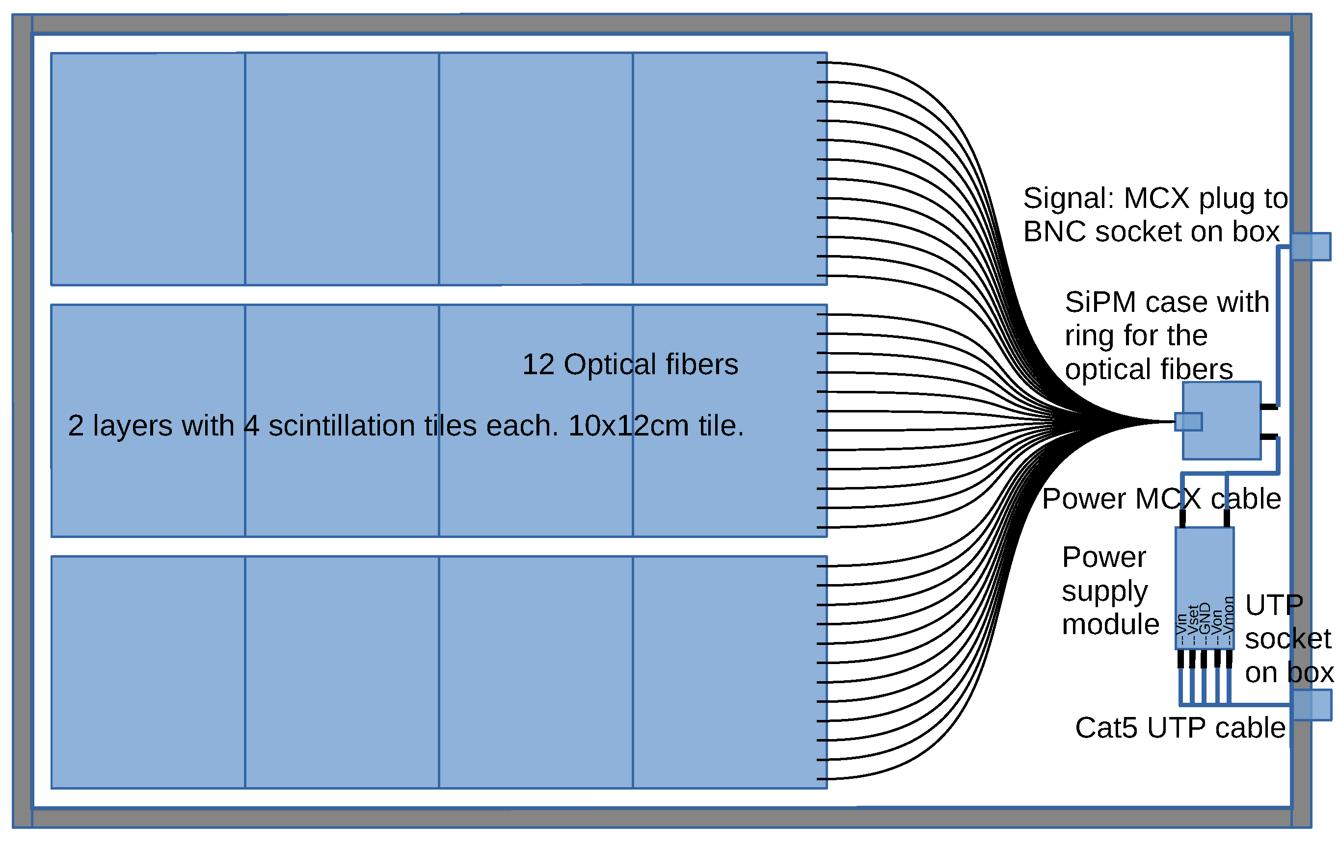
In
Figure 1 the original design schematic is presented. The enclosure of the detector unit’s components is a box with internal dimensions 40 × 65 × 4 cm. On the left of the schematic three rows of scintillation tiles are shown. Each row consists of two layers of four scintillation tiles per layer. Each row is traversed by twelve WLS fibers which are embedded in the grooves between the two layers of tiles. Each tile has dimensions 10 × 12 cm resulting in a detector unit’s effective scintillation area of 0.144 m
2. On the right of the schematic the SiPM coupled to the fibers, the power supply module and the signal and control connectors are also shown.
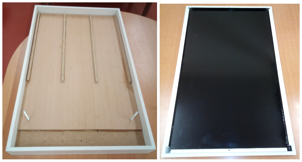
The scintillation tiles are placed on a wooden support structure made of 13 mm thick MDF, which is very rigid and easy to work. This MDF structure is also used as a support of the rest of the active components of the detector units. The support structure is placed in a box made of foam PVC 15 mm thick on the top and bottom and 10 mm thick on the sides. Foam PVC was chosen because is light weight and rigid enough to withstand lateral stresses without bending during the handling of the detector unit.
Figure 2 left shows the MDF support structure inside the PVC box before the placement of the scintillation tiles, WLS fibers and the rest active components. White foam PVC was chosen for aesthetic reasons, though it was later found that under strong illumination light could leak inside the box, crossing the 15 mm thickness of the material. To make the box light proof the internal surfaces of the PVC box were covered with black adhesive sheet (shown on
Figure 2 right). The lid of the box is fully detachable and employs four long rabbets for the fitting to the bottom part of the box, as shown on
Figure 2 right.
3. The Active Components of the Cosmics Detector Unit and the Construction
The active components of the detector unit include the scintillation tiles, the WLS fibers, the SiPM and its power supply.
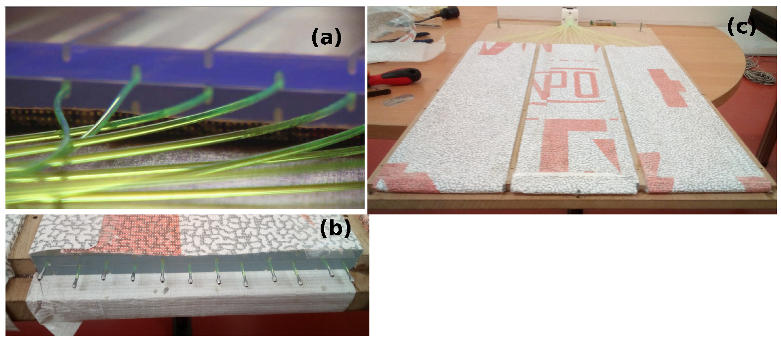
The scintillation tiles are made from molded scintillation material (SC-301). Each tile is 10 × 12 × 0.5 cm with grooves for the WLS fibers (see
Figure 3a). The scintillation material emits 8250 optical photons per MeV of deposited energy (55% the light output of anthracene), the main decay time is 2.4 ns, while the maximum emission is at 430 nm optical photon wavelength. The scintillation tiles are placed on the wooden support frame described in
Section 2, the WLS fibers are inserted in the grooves, and the overall is enclosed in a reflective Tyvek paper to enhance light output (see
Figure 3c). The WLS optical fibers are Bicron BCF-91A with an absorption length of 3.5 m, they are interfaced with the SiPM using a 3D printed construct described below, while at the opposite side they are clean cut and painted with reflective paint (see
Figure 3b).
The optical fibers must be permanently bent, as it is shown in
Figure 1,
Figure 3a and
Figure 4a. The type of fibers used show no significant loss when the bending radius is greater than 5 cm [
5]. This was taken into account during the design of the detector unit, and the minimum bending radius for the outer fibers is 7 cm.
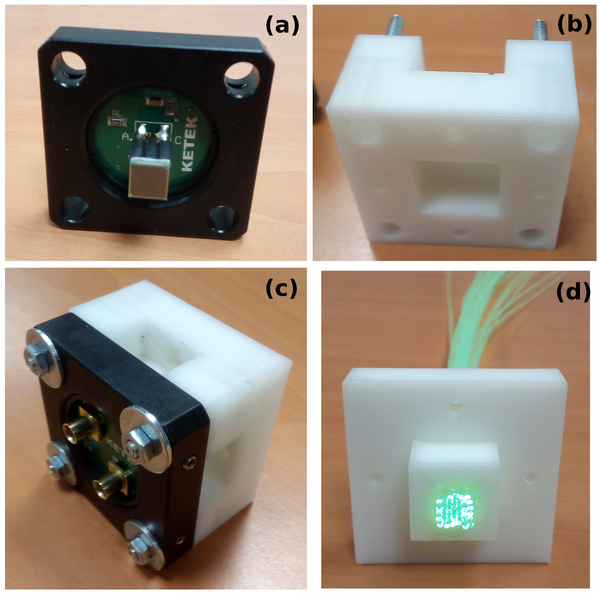
The photosensor used is a KETEK PM6650-EB silicon photomultiplier with sensor dimensions 6 × 6 mm. The SiPM is shown in
Figure 5a. It is attached to a small PCB board on a metal frame that is also provided by KETEK (The SiPM sensor is provided with pins that can be attached on the PCB board in two ways depending on the sign of output pulses required. In the first option the output pulses are positive, and a positive supply voltage is needed, while in the second option the output pulses are negative also using a negative supply voltage. For
Cosmics the second option was chosen since the detector units were first designed to work with existing electronics that require negative pulses on input.). The SiPM sensor consists of 14,272 micro cells of 50
m size. This SiPM has a maximum Quantum Efficiency 38% at 430 nm optical photon wavelength. It has a break down voltage of 27 V and it is operated at voltages 30–32 V. This SiPM was chosen due to its low cost and large sensor area that is adequate for coupling with the 1 mm diameter 36 WLS fibers.
To couple the WLS fibers with the SiPM we avoided using any adhesive between the SiPM and the fibers’ end. Instead, an interface structure was designed in two parts that fit to each other. The bottom part shown in
Figure 5b is used to hold the SiPM sensor in place and it is attached on the SiPM’s metal frame (see
Figure 5c). The top part shown in
Figure 5d holds the WLS fibers. The fibers are glued in the top part’s square hole and then are polished. By fitting the two parts together the polished end of the fibers is in perfect contact with the SiPM sensor without any risk of misalignment. The construction of the two parts was done by 3D printing using an ABS high density material.
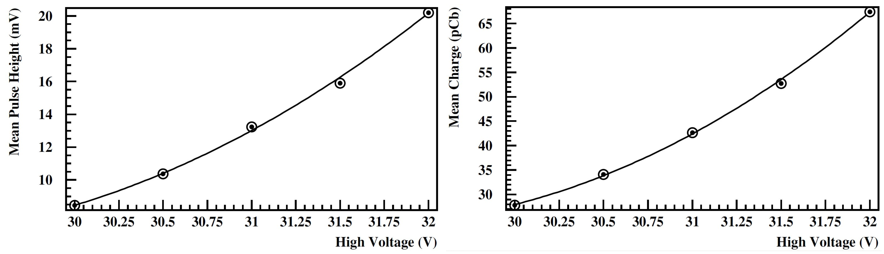
The power supply of the SiPM is the HMA-0.2N2.5-5 module from hivolt.de that outputs 0 to VDC voltage and is placed on the MDF support structure in the detector unit. The output voltage is adjusted linearly from 0 to VDC through a control input voltage of 0 to V. The safe operation of the SiPM requires supply voltages with absolute values less than 40 V. To protect the SiPM from accidentally applied higher voltages a 40 V zener diode was added in parallel to the output of the power supply module. The control voltage is provided through a USB DAC (Analog Output Module) LucidControl AO4–5 (With slight construction changes there is the option to avoid using the computer-controlled USB DAC module and the power supply module referenced, but instead use a simple and very cheap step down voltage regulator with a 36 VDC power supply. This option reduces the overall component cost of the Cosmics telescope by 350 Eur.). This module provides four independent analog outputs 0 to V and can thus control up to four detector units. Since the input control voltage of the power supply module must be in the range from 0 to V and is not internally protected in the module, a 2.5 V zener diode was added in parallel to the control input of the power supply module. The required power and control voltage is send to the detector unit through a UTP connector, while the SiPM output pulses are read through a BNC connector, both attached on the PVC box.
The choice of the power supply and DAC modules was based on the low cost and the required accuracy of the SiPM operating voltage. The accuracy of the supply voltage has been measured to be 0.1 V for outputs in the range 25 to 35 V. On the other hand, the sensitivity of the SiPM gain,
G, to changes in its operating voltage is
(this can be concluded from the
Figure 6 below). This results in a 5% gain accuracy which is adequate for the intended use of the
Cosmics detector.
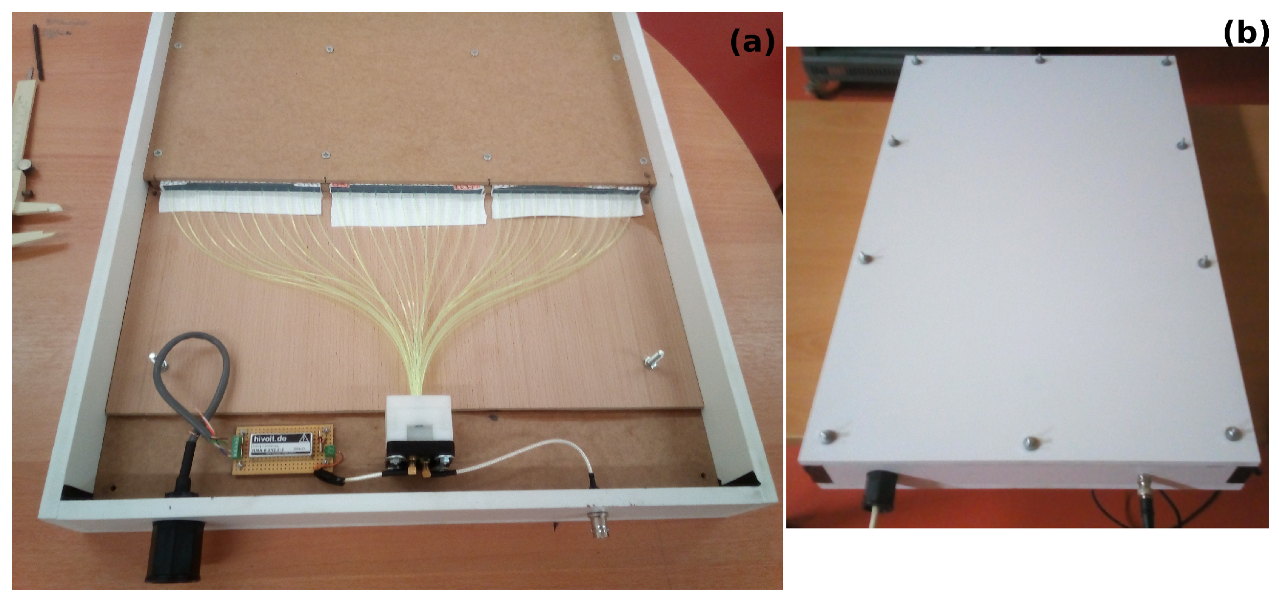
In
Figure 4a the detector unit with all the components in place is shown before closing with the lid. The lid is firmly attached to the box with ten through hole screws, nuts, and O-ring gaskets, as is shown in
Figure 4b. Between the box rim and the lid a rubber gasket is used for light proofing (not shown in the pictures). The light proofing of the finished detector is checked by comparing the current drawn by the SiPM in the dark and after illuminating with a strong light source.
4. Cosmics Telescope Calibration
The calibration procedure of the
Cosmics detector unit consists of the following steps [
6]:
Estimate the mean of the pulse height and charge distribution of the SiPM waveform when a Minimum Ionizing Particle (MIP) passes through the detector (A Minimum Ionizing Particle is a relativistic charged particle with energy loss rate due to ionization of the medium close to the minimum. Most of the atmospheric muons are MIPs, so when calibrating a detector to find its equivalent MIP response we are using atmospheric muons, a common practice in cosmic ray experiments.). This estimation must be done for each detector unit and for various power supply voltages to the SiPM. The experimental setup for this estimation is the placement of three
Cosmics detector units on top of each other. The top and bottom ones are used as a hodoscope (A hodoscope is a combination of at least two particle detectors that when both have signal in a narrow time window, we then know that a particle have passed through them.), and when the hodoscope is triggered the middle detector is read. In
Figure 6 the mean of the pulse height and charge distributions are shown as a function of the SiPM power supply voltage for one of the
Cosmics detector units. The reason for this calibration is twofold:
To avoid any bias during the data taking and event analysis all the detector units should have the same MIP pulse characteristics. For each unit, the power supply voltage should be adjusted separately so that all the units have the same mean of the MIP pulse height distribution. For the Cosmics detector units it was chosen to have this mean at 20 mV.
In EAS detector experiments it is common to express the deposited energy on the detector units during a shower event using the number of MIPS that would give the same deposited energy. To accomplish that we must be able to express the SiPM waveform’s charge in units of the charge of the response pulse to a MIP.
Estimate the appropriate parameterizations of the pulse arrival timing correction versus the pulse size. For the
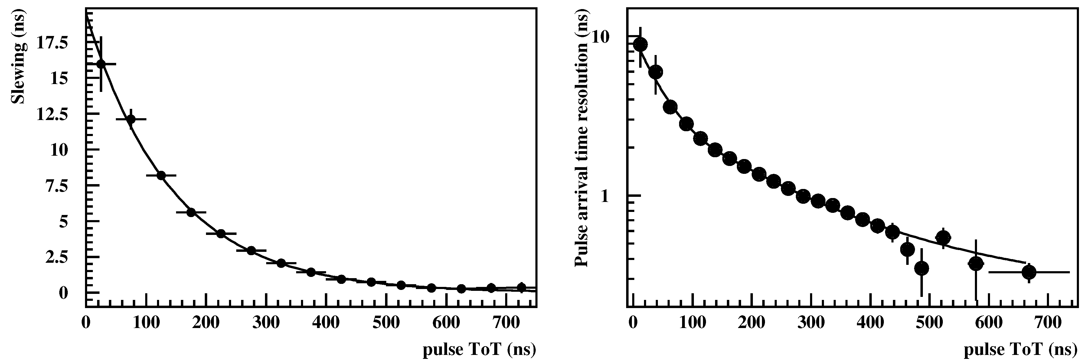
Cosmics we choose to have full digitization of the pulse of the SiPM using a low-cost USB oscilloscope. The oscilloscope is the Hantek 6254BD with four channels, 250 MHz bandwidth and a sampling rate of 1 GHz. The pulse arrival time is defined as the time when the pulse’s leading edge crosses the threshold of 6 mV (equivalent to 0.3 MIPs, since the MIP have a mean pulse height of 20 mV). However, this definition inserts a systematic error on the timing, since the pulse arrival timing does not depend only on the incident time of the EAS particle on the detector unit, but also on the pulse size (larger pulses have steeper leading edges). This effect (slewing) is corrected using parameterizations of the systematic timing shift versus the pulse size for each detector unit. The parameterizations are evaluated during the calibration by using the hodoscope setup referenced at step 1. To estimate the systematic timing shift of the middle detector unit we take the arrival time difference between this unit’s pulses and one of the hodoscope unit’s pulses (reference pulses) (Only when the reference pulses are large. The slewing timing shift decreases as the pulse size increases, so by comparing relative to the timing of a large reference pulse the result can be considered unaffected by the slewing effect of the reference pulse.). The procedure is repeated for every pulse size region of the middle detector unit, and an example result for a detector unit is shown in left plot of
Figure 7. In this plot the systematic timing shift is expressed as a function of the Time over Threshold (ToT) value of the pulse (this is the time interval where the pulse exceeds the threshold of 6 mV) (When the whole pulse is digitized there is the option to apply more sophisticated pulse arrival time estimations, e.g., fit the pulse with a standard shape or apply a constant fraction discriminator software algorithm on the digitized pulse, or use the inflection point of the rising edge of the pulse. All these methods are equivalent if the pulses follow a standard shape and only the pulse maximum (height) changes. Moreover, these methods define the pulse arrival time in a way independent of the pulse height. However, it was found that either the performance of these methods is limited due to the vertical resolution and dynamic range of the oscilloscope used, or they are too much CPU intensive and do not significantly improve the timing accuracy compared to the method referenced in the text.). In this step the synchronization of the detector units is also performed. The synchronization consists of estimating the relative time delays of the unit’s pulses due to possible differences in signal cables.
Estimate the pulse arrival time resolution versus the pulse size (ToT) for each detector unit. Since the EAS direction is estimated by the differences in the pulse arrival times of the detector units, this step is important to know the reconstruction errors of the estimated direction. The right plot of
Figure 7 shows this resolution versus the pulse size (ToT) for a detector unit.
5. EAS Reconstruction and Results
For the evaluation of the performance of the
Cosmics telescope three detector units were placed in the laboratory on the corners of an equilateral triangle with side 6.4 m. We used the Hantek 6254BD oscilloscope to acquire the data triggering on the signal from one detector unit at 20 mV (1 MIP) (This oscilloscope does not offer majority trigger logic.). Most of the events that were gathered were single muons passing through the detector unit used for triggering. The events where all the three detector units had a signal at least 1 MIP were reconstructed assuming the plane wave approximation of the shower front and using a simple triangulation method. Before the reconstruction, the appropriate corrections to the detector unit’s signal timing described in
Section 4, Step 2 were applied.
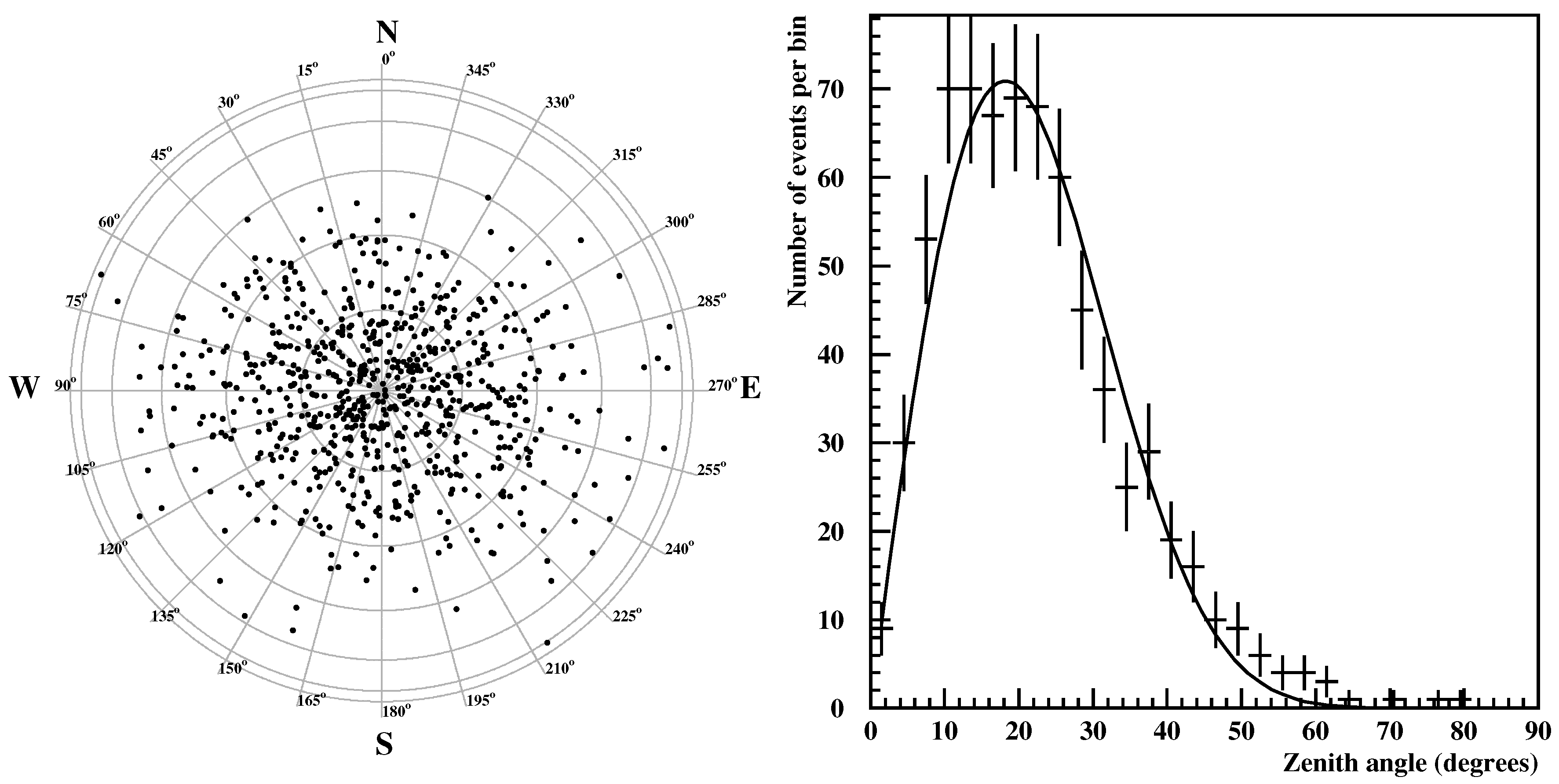
The results of the reconstruction are shown in
Figure 8. The left plot is a plane projection of the reconstructed directions, while on the right plot the zenith angle distribution is shown. This distribution is fitted with a function of the form
, where
. The found index from the fit is consistent with the one found when acquiring EAS with the HELYCON air shower array or similar detectors [
7,
8].
6. Discussion
The Cosmics cosmic ray telescope described above fulfills all the requirements to be used as an educational instrument that can be operated in high-school classrooms or university laboratories. It is low cost, portable, robust and does not employ dangerous high voltages or contains toxic materials. Moreover, its simplicity permits senior high-school students to participate actively in its construction, calibration, and operation. It has been designed using the experience gained during the development of the HELYCON air shower telescope. The calibration procedures and performance tests have been established and software packages have been developed for simulation, signal processing, event reconstruction, monitoring, and 3D event representation. Cosmics can also be used as a portable hodoscope for calibration of other air shower detectors, or for muon tomography measurements. In the immediate future it will be enriched with a radio frequency antenna that detects the RF signal emitted by very high energy air showers. The antenna will be designed having in mind the low cost and portability and it will be triggered by the detector units.
Author Contributions
Conceptualization, A.G.T. and A.L.; Data curation, A.G.T.; Formal analysis, A.G.T.; Funding acquisition, A.L.; Investigation, A.G.T.; Methodology, A.G.T.; Project administration, A.L.; Software, A.G.T.; Validation, A.G.T.; Writing–original draft, A.G.T.; Writing–review & editing, A.G.T. and A.L.
Funding
This research was funded by the Hellenic Open University Grant No. K 228:”Development of technological applications and experimental methods in Particle and Astroparticle Physics.”
Conflicts of Interest
The authors declare no conflict of interest.
References
- Manthos, I.; Gkialas, I.; Bourlis, G.; Leisos, A.; Papaikonomou, A.; Tsirigotis, A.G.; Tzamarias, S.E. Cosmic Ray RF detection with the ASTRONEU array. arXiv, 2017; arXiv:1702.05794. [Google Scholar]
- Tsirigotis, A.G. HELYCON: A Status Report. In Proceedings of the 20th European Cosmic Ray Symposium, Lisbon, Portugal, 5–8 September 2006. [Google Scholar]
- Leisos, A.; Avgitas, T.; Bourlis, G.; Fanourakis, G.K.; Gkialas, I.; Manthos, I.; Stamelakis, A.; Tsirigotis, A.G.; Tzamarias, S.E. The Hellenic Open University Cosmic Ray Telescope: Research and Educational Activities. EPJ Web Conf. 2018. [Google Scholar] [CrossRef]
- Leisos, A.; Tsirigotis, A.; Bourlis, G.; Petropoulos, M.; Xiros, L.; Manthos, I.; Tzamarias, S. HEllenic LYceum Cosmic Observatories Network: Status report and outreach activities. Universe 2019, 5, 4. [Google Scholar] [CrossRef]
- Gomes, A.; David, M.; Henriques, A.; Maio, A. Comparative study of WLS fibers for the ATLAS tile calorimeter. Nucl. Phys. B 1998, 61, 106–111. [Google Scholar] [CrossRef]
- Avgitas, T.; Bourlis, G.; Fanourakis, G.K.; Gkialas, I.; Leisos, A.; Manthos, I.; Tsirigotis, A.; Tzamarias, S.E. Deployment and calibration procedures for accurate timing and directional reconstruction of EAS particle-fronts with Helycon stations. arXiv, 2017; arXiv:1702.04902. [Google Scholar]
- Avgitas, T.; Bourlis, G.; Fanourakis, G.K.; Gkialas, I.; Leisos, A.; Manthos, I.; Stamelakis, A.; Tsirigotis, A.; Tzamarias, S.E. Operation and performance of a pilot HELYCON cosmic ray telescope with 3 stations. arXiv, 2018; arXiv:1801.04768. [Google Scholar]
- Elo, A.M.; Arvela, H. Direction distributions of air showers observed with the Turku air shower array. In Proceedings of the 27th International Cosmic Ray Conference, Hamburg, Germany, 7–15 August 2001. [Google Scholar]
© 2019 by the authors. Licensee MDPI, Basel, Switzerland. This article is an open access article distributed under the terms and conditions of the Creative Commons Attribution (CC BY) license (http://creativecommons.org/licenses/by/4.0/).


