Abstract
This paper presents a comprehensive statistical analysis of extremely/very low-frequency (ELF/VLF) whistler-mode waves observed within magnetic ducts (B-ducts) using data from NASA’s Magnetospheric Multiscale (MMS) mission. A total of 687 events were analyzed, comprising 504 occurrences on the dawn-side flank of the magnetosphere and 183 in the nightside magnetotail, to investigate the spatial distribution and underlying mechanisms of wave–particle interactions. We identify distinct differences between these regions by examining key parameters such as event width, frequency, plasma density, and magnetic field extrema within B-ducts. Using an independent two-sample t-test, we assess the statistical significance of variations in these parameters between different observation periods. This study provides valuable insights into the magnetospheric conditions influencing B-duct formation and wave propagation, offering a framework for understanding ELF/VLF wave dynamics in Earth’s space environment.
1. Introduction
Whistler-mode waves are important phenomena in plasma physics due to their ability to interact with high-energy electrons in the Earth’s radiation belt. These waves interact with particles through their cyclotron resonance and change their pitch angles, causing them to precipitate out of the magnetosphere [1]. By intentionally introducing controlled injections of whistler-mode waves from Earth or space into the magnetosphere, the presence of energetic particles in the Earth’s radiation belt can be reduced, thereby creating a safer environment for electronics and crews on space platforms [2,3].
As a notable characteristic, whistler-mode waves in the magnetosphere propagate along the ambient magnetic field, guided by field-aligned plasma density inhomogeneities referred to as the density ducts, which can be formed by the field-aligned density depletion (low-density duct or LDD), or enhancement (high-density duct or HDD). The presence of these ducts enables the propagation of whistler-mode waves over considerable distances in the Earth’s magnetosphere, including from one hemisphere to another, with minimal attenuation [4,5,6,7,8,9,10,11,12].
Recently, Ref. [13] have pointed out the occurrence of small-scale, localized packets of extremely low-frequency (ELF) waves within the inhomogeneities of the ambient magnetic field in the equatorial magnetosphere in the data gathered by the NASA Magnetospheric Multiscale Mission (MMS) satellites. These field-aligned inhomogeneities can be considered a high-magnetic duct (high-B duct or HBD) if they display magnetic enhancement, or a low-magnetic duct (low-B duct or LBD) if they are in the form of magnetic depletion. Extensive studies on whistler-mode waves trapping and propagation along magnetic ducts are presented in [13,14,15].
While the statistical investigation on density ducts has been carried out, e.g., [16], a statistical analysis of B-ducts is still lacking. This paper aims to fill this gap by systematically analyzing the statistical properties of B-ducts in different magnetospheric regions. By examining their distribution across key parameters, we provide an understanding of the occurrence, behavior, and significance of B-ducts, shedding light on their role in magnetospheric dynamics and plasma wave propagation. Recent studies have also highlighted the diverse roles of ULF waves in modulating magnetospheric wave activity and auroral phenomena, including their influence on chorus wave generation and their variability across planetary magnetospheres [17,18].
In this study, B-ducts are identified based on magnetic field inhomogeneities and localized variations in the total magnetic field magnitude , rather than individual vector components, to more reliably capture spatial structures and avoid misinterpretations due to dynamic field orientation. A structure is classified as a magnetic duct if the fluctuation in exceeds 20% relative to the smoothed local background magnetic field. This threshold is evaluated in conjunction with the presence of spatially and temporally correlated ELF/VLF whistler-mode wave packets. No fixed time window or minimum/maximum duct width was enforced during selection; instead, the identification relied on localized fluctuations that meet the amplitude criterion and coincide with wave activity. The background field is estimated using a moving average of over a local interval, ensuring that the reference field adapts to the ambient conditions without relying on external models.
For our statistical analysis, we use the actual magnetic field extrema observed within the ducts. Specifically, the maximum for high-B ducts (HBD) and the minimum for low-B ducts (LBD), rather than the deviation from the background. This choice reflects the physical field conditions relevant to wave propagation (e.g., determining electron cyclotron frequency), and avoids additional uncertainties associated with estimating or subtracting the background. Moreover, using extrema provides a consistent and interpretable measure across both duct types, enabling symmetric comparison of field enhancements and depletions.
The spatial scale of these structures is estimated using MMS-1 data, with width measurements derived from the spacecraft’s traversal through each event. This analysis does not attempt to resolve three-dimensional geometry, but focuses on the local cross-sectional scale observable from single-point measurements. The proximity of other MMS probes occasionally confirms the presence of the same structures, but our statistical survey is confined to the MMS-1 dataset for consistency, as our objective is to conduct a broad statistical characterization of magnetic duct properties.
2. Observation
This study uses data from NASA’s Magnetospheric Multiscale (MMS) mission, a constellation of four identical spacecraft launched in March 2015 to investigate the microphysics of magnetic reconnection, turbulence, and particle acceleration in the Earth’s magnetosphere [19]. The high temporal and spatial resolution of the MMS instruments makes them well-suited for studying fine-scale structures such as ELF wave packets and magnetic ducts.
To study B-ducts statistically, we analyzed data collected during two distinct periods of the MMS mission. During period A (in phase-1), spanning 1 to 7 March 2016, a total of 505 events associated with B-ducts were observed near the dawn-side flank of the magnetosphere. In period B (sampled from phase-2), conducted from 15 to 21 July 2017, 184 events were observed in the nightside magnetotail. Figure 1 shows examples of the correlation between the ELF wave packets localized in the magnetic structures formed as B-ducts observed by MMS-1 satellite in phase-1 (for Figure 1A) on March 06, 2016, from 23:25:44 to 23:27:59 UT, and in phase-2 (for Figure 1A’) from 1:44:20 to 1:47:40 UT on July 21, 2017. The color plot in the figures represents the power spectral density (PSD) of the component of the electric field, provided by the FIELDS Instrument Suite, and the electron number density is obtained by the MMS-1 FPI/DES instrument [20]. The magnetic field is measured by the MMS-1 Flux-Gate Magnetometer [21].
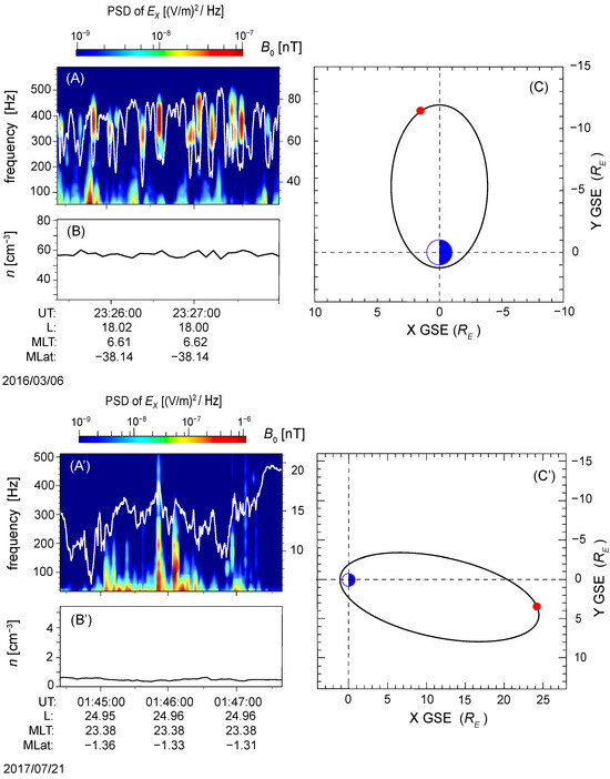
Figure 1.
ELF wave packets localized in the B-ducts observed by MMS-1 satellite in phase-1 on 6 March 2016, from 23:25:44 to 23:27:59 UT, and in phase-2 from 1:44:20 to 1:47:40 UT on 21 July 2017. Panels (A,A’) show the power spectral density (PSD) of component of the electric field in the GSE coordinate system of the satellite (shown with a color pallet) and background magnetic field (shown with the white line). Panels (B,B’) show the electron density measured by the MMS1 satellite. Panels (C,C’) show the trajectory and the location of MMS satellites (red dot) in the GSE X-Y plane on 6 March 2016 (19:00 UT), and 21 July 2017 (2:00 UT), respectively.
The spatial distribution of all detected events during both periods is summarized in Figure 2, illustrating the orbital coverage and regional separation of the two population samples. This analysis allows for a comparative investigation of B-duct formation and occurrence under varying plasma conditions and magnetospheric regions.
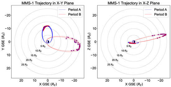
Figure 2.
Locations of the B-ducts detected by MMS-1 satellite in the equatorial magnetosphere in the study period in GSE X-Y, and GSE X-Z planes. Pink marks show the events detected in period A (1 to 7 March 2016) and purple marks indicate events detected during period B (15 to 21 July 2017). The orbit of MMS-1 during these periods is displayed by blue and red lines, respectively.
3. Descriptive Statistics Analysis
Throughout this study, we perform a statistical analysis to compare the B-duct counts across various parameters, such as event width, frequency, plasma density, and magnetic field extrema (maximum of B for HBD and its minimum for LBD) inside B-ducts. To assess whether significant differences exist between Periods A and B, we employ the independent two-sample t-test [22]. The analysis includes descriptive statistics, followed by the computation of the t-statistic and p-value, ensuring a robust evaluation of differences between the groups under investigation.
3.1. Independent Two-Sample t-Test
The independent two-sample t-test is a fundamental statistical tool used to determine whether there is a significant difference between the means of two independent groups. This test evaluates the null hypothesis that the means of the two groups are equal, providing insights into whether the observed differences are statistically significant or attributable to random variations [23]. In other words, it compares the observed difference between sample means to the variability within the samples, quantified through the t-statistic. The corresponding p-value provides a measure of statistical significance, allowing us to determine whether the observed difference is likely to be due to random chance [24].
3.1.1. t-Statistic Calculation
The t-statistic quantifies the difference between the means of two independent groups relative to their variability and sample sizes. In this study, we assume the two groups have unequal variances and use Welch’s t-test, which does not require the assumption of equal population variances. The t-statistic is calculated as
where
- and are the sample means of the two groups, e.g., period A and B event counts.
- and are the sample variances of the two groups, which measure the spread or variability within each group.
- and are the sample sizes of the two groups, reflecting the number of observations within each dataset.
A larger t-statistic indicates that the difference between the group means is large relative to the variability within the groups, increasing the likelihood of statistical significance. Conversely, a smaller t-statistic suggests that the group means are similar relative to the observed variability [25].
3.1.2. p-Value
The p-value is a measure of the probability of obtaining the observed test results under the null hypothesis (i.e., assuming the group means are equal). It serves as a key indicator of statistical significance [23].
- High p-value (): Suggests that the observed differences are likely due to random chance, and there is no significant difference between the means.
- Low p-value (): Indicates that the observed differences are unlikely to be due to chance, and the means of the two groups are significantly different.
The p-value provides a quantitative basis for accepting or rejecting the null hypothesis. If the p-value is below the chosen significance level (e.g., 0.05), we reject the null hypothesis and conclude that the group means differ significantly.
3.1.3. Equal Variance Assumption
The independent two-sample t-test assumes that the variances of the two groups are either equal or different. This impacts the specific type of t-test applied,
- Standard t-test (Equal Variances): Assumes the variances of the two groups are equal.
- Welch’s t-test (Unequal Variances): By default, Welch’s t-test is used when the variances or sample sizes of the two groups differ. This version of the test is more robust and reduces the risk of inaccurate conclusions under unequal variance conditions [26].
4. Magnetic Ducts’ Distribution Analysis
In this section, the statistical characteristics and patterns of B-ducts observed during the two study periods are presented. By analyzing the width, frequency, and spatial distribution of events, we aim to identify underlying trends and relationships between key parameters of B-ducts such as the ratio, magnetic extrema, and density.
4.1. Width Distribution
The cross-sectional width of B-ducts is determined using MMS Mission Ephemeris Coordinates (MEC) by identifying the spatial extent of the localized magnetic field structure as the spacecraft traverses it. This width corresponds to the distance between entry and exit points of the duct, based on sharp magnetic field gradients and consistent duct morphology.
Figure 3 shows the distribution of B-duct counts with respect to their width in km. The histogram shows the actual observed event widths, while the green line represents a fitted normal distribution curve based on the mean and standard deviation of the data. It is important to note that this normal distribution fit is provided solely for visual comparison, emphasizing deviations from symmetry and highlighting the skewness inherent in the observed data.
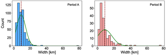
Figure 3.
Distribution of B-duct counts to their width in km. The histogram shows the actual observed event widths for the period A (left), and period B observed events (right). The green line represents a fitted normal distribution curve based on the mean (red dashed line) and standard deviation of the data.
Period A events, occurring on the flank of the magnetosphere, have a mean width of 9.02 km and show a wider distribution, indicating greater variability in B-duct widths. In contrast, period B events, observed in the magnetotail, have a slightly lower mean width of 8.85 km and exhibit a more peaked distribution, reflecting narrower B-ducts.
The skewness analysis shows that the period A dataset has a skewness of 4.93, while the period B dataset has a skewness of 3.82. Both datasets exhibit positive skewness, indicating that the distributions have a longer right tail. This suggests the presence of wider B-ducts that are less frequent but extend the distribution to the right. The flank events show a higher skewness (4.93), implying a stronger asymmetry compared to the tail events (3.82). This positive skewness could suggest the occurrence of rare but significantly wider B-ducts, particularly in the period A data.
4.2. Frequency Distribution
The characteristic frequency of waves within each B-duct is determined using the power spectral density (PSD) of the component of the electric field, provided by the FIELDS Instrument Suite. The dominant wave frequency is identified as the frequency (or frequency band) corresponding to the peak PSD value within the time interval when the spacecraft is traversing the duct.
The frequency distribution of waves trapped within observed B-ducts across different magnetospheric regions reveals critical insights into the underlying plasma dynamics. Figure 4 visualizes this distribution. Table 1 provides a detailed statistical analysis of B-duct counts versus frequency for the datasets from periods A and B. The analysis highlights significant differences in central tendency, variability, and distribution shape, offering valuable perspectives on the frequency profiles and the physical processes governing these phenomena.
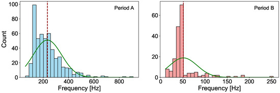
Figure 4.
Distribution of B-duct counts vs. the frequency in Hz for period A (left), and period B (right). The green line represents a fitted normal distribution curve based on the mean (red dashed line) and standard deviation of the data.

Table 1.
Event counts vs. frequency distribution statistical analysis.
The central tendency shows that the trapped whistler-mode waves in B-ducts during period A have much higher mean and median frequency peaks than those observed in period B. Flank events have a mean frequency peak of 233.35 Hz, far higher than the 54.44 Hz for magnetotail events. Similarly, the median frequency peak for the flank events is 213 Hz, compared to just 44 Hz for magnetotail events. This suggests that flank B-ducts trap higher frequency waves compared to magnetotail B-ducts. While frequency alone does not determine wave energy, the observed shift may reflect different plasma conditions or wave generation mechanisms influencing wave–particle interactions in these regions of the magnetosphere.
While the absolute standard deviation for Period A events (111.49 Hz) is higher than that for Period B (53.75 Hz), the standard deviation relative to the mean reveals a different picture. The relative standard deviation is approximately 47.8% for Period A and 98.7% for Period B, indicating that frequency values in the magnetotail (Period B) are more dispersed when normalized to the mean, i.e., they exhibit higher relative variability. However, the absolute frequency range is broader for flank events (60 Hz to 910 Hz) compared to magnetotail events (11 Hz to 644 Hz), reflecting a wider spread in raw values.
This distinction suggests that while magnetotail events show greater relative dispersion due to their low mean frequency, flank events (Period A) demonstrate more diverse wave characteristics in absolute terms. The wider spread of high-frequency values in the flank may indicate the presence of multiple wave modes or more variable local plasma conditions. In contrast, magnetotail whistler events are concentrated at lower frequencies, consistent with more homogeneous wave activity in the tail region.
The skewness analysis indicates the skewness of 1.73 for period A events. The data is positively skewed (right-skewed), suggesting a longer tail on the right side of the distribution. It also shows the skewness of 7.85 for period B events. The datasets are highly positively skewed, indicating a significant right-skew with a pronounced tail. This indicates that both datasets have frequent occurrences of ELF waves with a few higher-frequency events acting as outliers.
The high kurtosis, especially for magnetotail events, suggests the presence of extreme outliers. This could be due to rare but intense wave–particle interactions in the tail region, leading to occasional higher-frequency events.
In addition, both datasets are leptokurtic, but the magnetotail events have an extremely high kurtosis value (78.72), suggesting a distribution with very heavy tails and a high likelihood of outliers. The Shapiro-Wilk test confirms that both datasets do not follow a normal distribution, with p-values well below 0.05.
In conclusion, the flank events exhibit higher frequency peaks with greater variability, possibly indicating stronger and more diverse wave activity. Magnetotail events are dominated by lower frequencies but have a significant number of extreme outliers, suggesting occasional high-frequency disturbances, likely influenced by different plasma dynamics in the magnetotail region.
The findings align with known differences in the magnetospheric environment. The flank region is influenced by a variety of wave–particle interactions, resulting in a broader frequency range and higher energy events. Such characteristics have been observed in studies of the dawn and dusk flanks, where electromagnetic ion cyclotron (EMIC), magnetosonic, and whistler-mode waves are more prevalent due to enhanced plasma instabilities and compressional effects [27,28]. The magnetotail region typically hosts lower-frequency wave phenomena, but sporadic higher-frequency events may occur due to sudden dynamic processes such as reconnection or plasma injections. These transient processes have been associated with bursty bulk flows and dipolarization fronts, which can generate localized wave enhancements [29,30].
4.3. Frequency vs. B-Duct Type Distribution
The frequency distribution of waves trapped within HBDs and LBDs provides valuable insights into the dynamic processes of the magnetosphere. By analyzing the occurrence of the type of B-duct events during periods A and B, we explore how these duct types are distributed in terms of the frequencies of trapped waves across distinct regions, providing insights into the magnetospheric processes that shape their occurrence and behavior.
Figure 5 shows the distribution of B-duct types (high or low B-duct) vs. frequency of the trapped whistler-mode wave in the ducts in periods A and B. Analysis shows that period A (on the flank) has a significantly higher number of events, with 328 LBD events and 175 HBD events. This means that in period A, almost 65% of the events are LBD events, while 35% are HBD events.
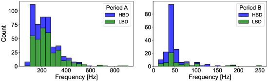
Figure 5.
Distribution of B-duct types (HBD or LBD) versus frequency of trapped whistler-mode waves for period A (left) and period B (right).
The magnetotail region shows fewer events, with 53 (29.12%) LBD and 129 (70.88%) HBD events. The lower count of LBD events compared to HBDs may indicate different generation mechanisms or wave–particle interactions specific to the magnetotail environment.
Figure 6 shows the frequency distribution of HBD and LBD events during periods A and B. The box plots illustrate the median frequencies, interquartile ranges, and variability for each duct type within the two observation periods.
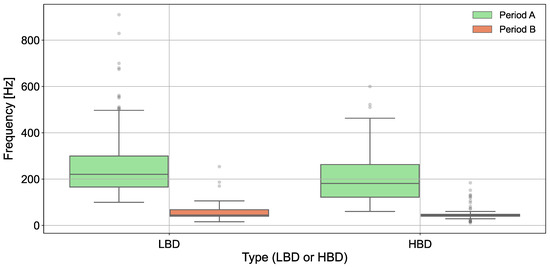
Figure 6.
Frequency distribution of HBD and LBD events observed during period A (green) and period B (red). The box plots highlight the median, interquartile range, and variability in frequency for each duct type and observation period, with outliers represented as circles.
As shown in Table 2, period A dataset shows that HBD events have a mean frequency of 209 Hz, with a wide frequency range (60 Hz to 600 Hz). LBD events have a slightly higher mean frequency of 246 Hz, extending up to 910 Hz. The broad frequency distribution indicates a diverse range of wave–particle interactions, or suggests the presence of stronger magnetic fluctuations in the flank region.
Table 2.
Comparison of frequency of whistler-mode waves trapped inside HBDs and LBDs in period A and B.
In period B, HBD events have a much lower mean frequency of 47.8 Hz, with most frequencies falling below 184 Hz. LBD events have a mean frequency of 59.4 Hz, with a maximum of 254 Hz. The lower frequencies in the magnetotail region reflect a plasma environment with different density and magnetic field conditions, affecting wave propagation and interaction.
Overall, the flank region exhibits a higher number and broader range of events, with significantly higher frequencies compared to the magnetotail region. This suggests
- stronger wave–particle interactions and potentially higher plasma densities or magnetic irregularities in the flank;
- a possible increase in electron cyclotron resonance in the flank, as indicated by higher mean frequencies.
The magnetotail region’s lower frequencies and fewer events point towards a quieter plasma environment, where whistler-mode waves are less energetic or less frequently generated.
4.4. Plasma Density Distribution
Electron plasma density analysis provides insight into the plasma environments where whistler-mode waves were observed. By comparing the density distributions of the B-duct events on the flank and the magnetotail, we can infer the underlying plasma conditions in these regions of the magnetosphere. Figure 7 shows the distribution of B-duct counts and their electron plasma density in periods A and B, with the mean density of 55.84 for period A, and 0.26 for period B.
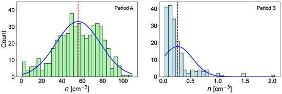
Figure 7.
Distribution of B-duct counts to the plasma density (n) in for period A (left), and period B (right). The blue line represents a fitted normal distribution curve based on the mean (red dashed line) and standard deviation of the data.
The density values in the flank region show a slight negative skew (left-skewed) with a skewness of −0.32. A slight left skew indicates that most of the density values are higher, with a few lower-density outliers. This suggests that the plasma density for B-ducts in the flank region tends to be relatively high, but there are occasional events with lower densities. The distribution is closer to being symmetric, implying a relatively stable plasma environment with less extreme variability in density compared to the magnetotail region. However, the presence of higher densities in the flank region may be related to the influence of the solar wind, which compresses the magnetosphere’s flanks, increasing plasma density.
Density values in the magnetotail region show a strong positive skew (right-skewed) with a skewness of 3.09. The significant right skew indicates that for most B-ducts, the density values are low, but there are some higher-density outliers. This is characteristic of the magnetotail, where low-density plasma is prevalent, and high-density events are less common but can occur due to dynamic processes. The occasional higher-density spikes could be caused by plasma injections or reconnection events, which temporarily increase the local density.
The differences in plasma density observed for B-ducts reflect the distinct characteristics of magnetospheric regions. These findings help explain the behavior of whistler-mode waves’ interaction with B-ducts, shaped by the local plasma environment. The results indicate that B-duct events are more common in denser plasma within the flank region, whereas the tail region, with its more tenuous plasma, occasionally experiences disruptions caused by dynamic processes.
The differences in plasma density observed for B-ducts reflect the distinct characteristics of magnetospheric regions. These findings help explain the behavior of whistler-mode waves interacting with B-ducts, shaped by the local plasma environment. The results indicate that B-duct events are more common in denser plasma within the flank region, whereas the tail region, with its more tenuous plasma, occasionally experiences disruptions caused by dynamic processes. Processes such as magnetic reconnection or plasma burst flows can temporarily modify the magnetic field geometry and plasma density, thereby disturbing or suppressing stable duct formation. Consequently, whistler-mode waves in the magnetotail can be trapped and experience guided propagation within the created B-ducts.
4.5. Magnetic Field Extrema Distribution
The analysis of magnetic field extreme data—i.e., maximum background magnetic field for HBD and minimum for LBD, provides a comparative framework for interpreting wave–particle interactions in the distinct magnetic environments of the flank and magnetotail regions where B-ducting occurs. Figure 8 and Figure 9 illustrate the distribution of HBD and LBD counts and magnetic extrema for periods A and B, revealing a mean magnetic peak of 63.33 nT for period A and 15.33 nT for period B. This disparity underscores the distinct magnetic characteristics of these regions. Table 3 provides a detailed statistical analysis of B-duct counts vs. frequency distribution for the datasets from periods A and B.
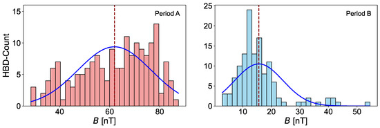
Figure 8.
Distribution of HBD counts relative to the magnetic field maximum values inside HBDs in nT for period A (left), and period B (right) Blue line represents a fitted normal distribution curve based on the mean (red dashed line) and standard deviation of the data.
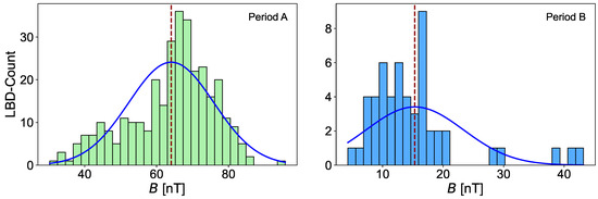
Figure 9.
Distribution of LBD counts relative to the magnetic field minimum values inside LBDs in nT for period A (left), and period B (right). Blue line represents a fitted normal distribution curve based on the mean (red dashed line) and standard deviation of the data.
Table 3.
Event counts vs. frequency distribution statistical analysis.
For the maximum magnetic field measured inside HBDs in period A, the calculated skewness is −0.41 (Slightly negatively skewed). The negative skew indicates a minor bias toward higher magnetic peak values, with a tail extending toward lower values. This reflects relatively stable magnetic conditions with fewer lower-B intensity events. For LBDs, the skewness is −0.58 (Slightly negatively skewed). The slightly stronger negative skew suggests a distribution that is dominated by higher magnetic peaks but with some rare dips to lower values. The negative Kurtosis −0.84 (Platykurtic) shows that the HBD distribution in the flank of the magnetosphere is flatter than a normal curve, indicating fewer extreme outliers and a more even spread around the mean.
In the flank region, HBD events demonstrate consistent magnetic field conditions with occasional lower-B dips. These may result from transient compressions or stable solar wind interactions with the magnetosphere. For LBD events, the slightly stronger skewness implies that most events occur under higher magnetic field conditions, with occasional reductions likely tied to temporary magnetospheric fluctuations or localized disturbances. Nearly normal Kurtosis (−0.10) shows that the distribution is close to normal, with a balance between high and low values. This suggests a steady environment for LBD events in the flank of the magnetosphere with rare extreme values.
The overall characteristics of the flank region imply that B-ducts are influenced by stable and relatively strong magnetic fields for both types, with variability being slightly more pronounced in LBD events. These conditions create favorable environments for whistler wave trapping in LBDs.
For the maximum magnetic field measured inside HBDs in period B, the calculated skewness is 2.03 (strongly positively skewed). The strong positive skew indicates a distribution dominated by low magnetic peak values, with a long tail toward higher peaks. This reflects occasional high-intensity outliers in the magnetotail environment. For LBDs, the skewness is 1.95 (strongly positively skewed). Similar to HBDs in the magnetotail, the positive skew indicates a predominance of low magnetic peaks, with rare intense events extending the tail. Leptokurtic kurtosis of 5.03 also shows that the distribution has heavy tails and a sharp peak, indicating the presence of frequent extreme outliers. These high magnetic peaks could result from transient and dynamic processes like magnetic reconnection.
In the magnetotail region, LBD events are characterized by weaker magnetic fields with occasional high peaks, likely associated with dynamic processes such as magnetic reconnection or plasma injections. LBD events exhibit a similarly skewed distribution, dominated by low-intensity conditions but with rare transient enhancements due to localized reconnection events or plasma flows. Similar to HBDs in the magnetotail, the leptokurtic kurtosis of 4.00 shows that the distribution has heavy tails and a sharp peak, suggesting frequent extreme outliers. This aligns with transient and sporadic enhancements in magnetic fields in the magnetotail region.
4.6. B-Ducts vs. Distance Distribution
Whistler-mode waves B-ducting is highly influenced by the local plasma environment, particularly by the electron density and magnetic field strength. The differences in distance distributions between the flank of the magnetosphere and magnetotail events imply distinct propagation environments. Thus, the analysis of B-ducts distributions in terms of their distances from the Earth’s center (in Earth radius, ) provides important insights into the spatial relationship between these events and the plasma environment, such as the plasmapause and magnetopause.
The plasmapause is the boundary where the density of cold plasma in the Earth’s magnetosphere decreases sharply. It spans between . It plays a critical role in wave propagation, particularly for whistler-mode waves in density ducts which are sensitive to changes in plasma density [16].
The magnetopause is a dynamic boundary in space that marks the outer edge of Earth’s magnetosphere, where the planet’s magnetic field meets and interacts with the solar wind. It acts as a shield, deflecting charged particles from the Sun and preventing them from directly impacting Earth’s atmosphere [31]. The position and shape of the magnetopause are highly variable, influenced by changes in solar wind pressure, typically ranging from approximately on the dayside, and can extend much farther, up to 60–100 , on the nightside in the magnetotail [32,33].
Figure 10 shows the distribution of observed B-ducts and their distance from the Earth in periods A and B.
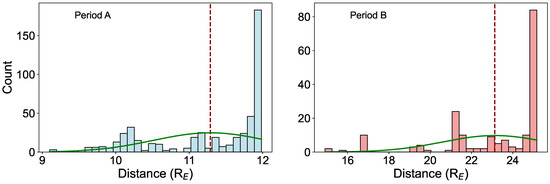
Figure 10.
Distribution of B-duct vs. their distance from the Earth in for B-duct events in period A (left), and period B (right). Green line represents a fitted normal distribution curve based on the mean (red dashed line) and standard deviation of the data.
The mean distance for B-ducts in the flank of the magnetosphere is observed to be around 11.29 , with a range spanning from 9.10 to 11.98 . This range suggests that many of these events are detected beyond the typical plasmapause location, which generally ranges from 4 to 6 under quiet geomagnetic conditions. The distribution’s skewness, with a tail extending towards larger distances, indicates the presence of some events occurring well over the nominal magnetopause boundary ).
The mean distance for magnetotail events is notably larger, at 23.13 , with a broad distribution ranging from 14.90 to 25.17 . This suggests that magnetotail B-duct events are occurring well outside the typical plasmapause boundary, likely in the plasma sheet or lobe regions of the stretched magnetosphere. The distribution’s symmetry, with a slight right skew, points to the influence of dynamic magnetospheric processes such as tail stretching or plasmasheet thinning, which can extend the regions of enhanced wave activity further from the Earth.
4.7. Ratio Distribution
While Section 4.2 analyzes general frequency characteristics of whistler-mode waves within B-ducts, here we specifically focus on the normalized frequency ratio (). Generally, whistler-mode waves are classified into two categories based on their frequencies: low-frequency (LF) whistlers, where , and high-frequency (HF) whistlers with . This distinction is physically significant, as the behavior and properties of whistlers differ between the LF and HF regimes.
Figure 11 shows the distribution of B-duct counts and ratio in periods A and B. The analysis of the ratio for the flank and magnetotail environments, showcased in details in Table 4, reveals distinct characteristics that provide insight into the nature of whistler-mode wave events in these two regions of the magnetosphere. Notably, almost all (99.6%) of observed events during period A are classified as LF whistler-mode waves. In contrast, the magnetotail region exhibits a few outliers in the HF regime (3.30%), suggesting variations in wave behavior that may be influenced by local plasma conditions.
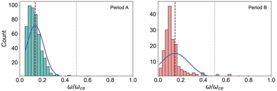
Figure 11.
Distribution of B-duct vs. the trapped whistler-mode wave’s distribution in period A (left), and period B (right). Blue line represents a fitted normal distribution curve based on the mean (red dashed line) and standard deviation of the data. Gray dotted line shows the HF-LF threshold at .
Table 4.
Statistical Analysis for distribution in period A and B.
The mean ratio is slightly higher in the magnetotail region compared to the flank. This suggests that the wave frequencies are closer to the in the magnetotail region. This is attributed to the different plasma environments in the magnetotail, leading to a relatively higher wave frequency. The standard deviation is significantly higher in the magnetotail, indicating greater variability in the ratio. This could reflect a more turbulent or heterogeneous plasma environment in the magnetotail, where wave properties are less consistent than in the flank region.
Both distributions are positively skewed, meaning there is a long tail of higher ratio values. However, the skewness is more pronounced in the flank dataset. The high skewness in the flank suggests that while most events have a low ratio, there are a few events with significantly higher ratios. This could indicate occasional strong wave activity or wave–particle interactions with the higher wave frequency. The lower skewness in the magnetotail indicates a more balanced distribution, but the positive value still reflects the presence of outliers with higher ratios.
Kurtosis measures the ’tailedness’ of the distribution. Both datasets have high kurtosis, indicating the presence of heavy tails and sharp peaks, with the flank dataset showing an extremely high kurtosis. The high kurtosis in the flank suggests that the distribution is highly peaked, with most values concentrated around the mean, but with a few extreme outliers. This could be a sign of occasional, intense wave–particle interactions in the flank region that lead to higher ratios. The magnetotail dataset, while still showing high kurtosis, is less extreme, indicating a broader, less peaked distribution. This could be consistent with a more varied wave environment in the magnetotail.
The minimum values in both datasets are relatively low, indicating that there are events where the wave frequency is significantly lower than 0.5. The maximum values in both datasets are close (around 0.8), suggesting that in the most extreme cases, the wave frequency can get quite close to the . The existence of such HF events in the magnetotail with a very dilute plasma environment can be associated with dynamic processes such as magnetic reconnection or plasma injections.
4.8. Magnetic Peak vs. Density Peak Distribution
Figure 12 shows the combined heatmap plot, providing a detailed visualization of the relationship between plasma density, magnetic field extrema inside the B-duct, and frequency of the trapped wave during periods A and B. It reveals distinct clustering patterns and distributions that reflect the varying physical conditions in these magnetospheric regions. Each heatmap demonstrates how plasma density and magnetic field extremum influence frequency distributions.
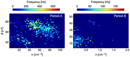
Figure 12.
Heatmaps showing the frequency of whistler-mode waves, plasma density, and magnetic field extrema distribution in the observed B-ducts during Period A (left), and Period B (right). Separate colorbars for each heatmap show the frequency distributions across the two periods.
4.8.1. Period A Analysis
In the flank region, the data exhibits significant clustering within moderate to high plasma densities, ranging from approximately 20 to 75 . The magnetic field extremum values also show a wide range, predominantly between 50 and 85 nT. This indicates that the plasma in the flank region is characterized by both higher densities and stronger magnetic field perturbations. Centrality of the data in this heatmap is evident in the concentrated regions of high frequency, particularly within bins where the density exceeds 40 and magnetic field values approach the upper limits.
The frequency distribution shows a dominance of higher frequencies, often exceeding 300 Hz, tightly clustered in regions where plasma density and magnetic field strength are both elevated. The clustering suggests that these conditions create an environment conducive to strong wave–particle interactions, where energetic particles interact with whistler-mode waves.
4.8.2. Period B Analysis
This heatmap demonstrates a remarkable different clustering and distribution pattern. Plasma densities are much lower, predominantly clustering in the range of 0.1 to 0.5 . Similarly, magnetic field strength values are significantly weaker, clustering around 10 to 20 nT.
The frequency distribution is predominantly concentrated in lower frequencies, ranging between 25 Hz and 50 Hz. These frequencies exhibit clustering in regions where plasma densities are at their lowest and magnetic field strengths remain within a narrow range. Unlike the flank data, the centrality of data in the magnetotail heatmap is located in these low-frequency, low-density, and low-magnetic-field regions, reflecting weaker wave–particle interactions. The distribution of data points suggests that the magnetotail is a relatively stable and less dynamic region, consistent with its location downstream of the primary solar wind–magnetosphere interaction zone.
In both periods, the heatmaps show internal clustering, where B-duct events tend to group around specific combinations of plasma density and magnetic field strength. These clusters suggest the existence of preferred conditions for wave trapping—such as moderate-to-high density and field values—within each region, rather than a continuous or random distribution. This behavior highlights the structured nature of wave-–duct interactions in both the flank and magnetotail environments.
4.9. Magnetic Field and Plasma Density Conditions for Whistler Events
To understand the typical environmental conditions under which whistler-mode waves occur in different regions of the magnetosphere, we analyzed the distribution of events in the magnetic field–plasma density parameter space. Figure 13 shows 2D kernel density estimates (KDEs) of event occurrence as a function of extremum magnetic field and corresponding plasma density for two distinct regions. Each panel presents a separate KDE-based heatmap where color intensity represents the estimated relative density of events. The use of KDE smooths the spatial distribution, highlighting the most probable conditions of occurrence rather than discrete event counts.
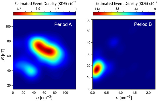
Figure 13.
2D kernel density estimation (KDE) heatmaps showing the distribution of whistler-mode wave events in the space of extremum magnetic field (Extremum_Bt_GSE) vs. corresponding plasma density. Left: events in the flank region; right: events in the magnetotail. The color scale indicates relative KDE intensity using the jet colormap. Each region is plotted independently with its own colorbar in scientific notation.
In the flank region, whistler events tend to occur across a broad range of magnetic field strengths (∼40–100 nT) and relatively high plasma densities (10–80 ). The KDE surface is more diffuse in this case, suggesting that flank whistlers are associated with moderately strong magnetic fields and dense plasmas, likely originating near the plasmapause or in boundary layer regions. In contrast, the magnetotail region reveals a sharply localized distribution at lower magnetic fields (∼5–25 nT) and very low densities (<1 ), characteristic of the plasma sheet or magnetotail lobes. This clear distinction suggests different physical regimes for wave generation where the tail may favor bursty reconnection and thin current sheets, while the flank supports interactions in more stable, denser environments.
4.10. Final Statistical Remarks
To quantitatively assess the differences between the two observation periods, Period A (dawn-side flank) and Period B (nightside magnetotail), we applied two complementary statistical analyses. First, the Shapiro–Wilk test was used to evaluate the normality of the distributions for key B-duct parameters. Second, Welch’s two-sample t-test was used to compare the mean values of these parameters between the two regions, as it is robust to unequal variances and non-normal data.
Table 5 presents the Shapiro–Wilk test results. Most variables showed significant deviations from normality in at least one of the periods, justifying the use of Welch’s t-test for further comparison. In particular, wave frequency, electron density, and the ratio were found to be non-normal in both datasets. These p-values are derived from the Shapiro–Wilk test and are used solely to assess normality, not differences in group means.
Table 5.
Shapiro–Wilk test results for normality of B-duct parameters in Period A and Period B. A p-value < 0.05 indicates a statistically significant deviation from normality.
Table 6 summarizes the results of the Welch’s t-test. In contrast to Table 5, the p-values reported here are obtained from Welch’s t-test and indicate the significance of differences between group means. Statistically significant differences () were found between the two regions for frequency peak, plasma density, and magnetic field extrema. These findings reinforce the interpretation that whistler-mode wave activity in the flank is associated with higher frequencies, denser plasma, and stronger magnetic field variations. In contrast, the magnetotail exhibits lower-frequency wave activity in more tenuous magnetic and plasma environments. Interestingly, the mean width of the observed B-ducts did not differ significantly between the two regions (), suggesting that the physical scale of these structures remains relatively constant across diverse plasma environments.
Table 6.
Welch’s t-test results comparing B-duct parameters between Period A and Period B. Values are reported as mean ± standard deviation. Here, W stands for for width [km], f for the wave frequency peak [Hz], n for electron plasma density , B for magnetic field extrema [nT], for normalized wave frequency.
We note that, although the number of detected events is reported per period, these values are not normalized by transit time or spacecraft trajectory length. The periods have been defined to ensure comparable orbital coverage, and our conclusions are primarily based on the physical and statistical properties of the events, rather than on raw occurrence rates.
Together, these statistical results provide quantitative confirmation and support for the descriptive trends discussed in earlier sections, thereby strengthening the conclusion that B-duct formation and wave propagation are regionally distinct in the Earth’s magnetosphere.
5. Conclusions
To study B-ducts statistically, we analyzed data collected during two distinct periods of the MMS mission. During period A, spanning 1 to 7 March 2016, a total of 505 events associated with B-ducts were observed near the dawn-side flank of the magnetosphere. This region, where solar wind interactions stretch magnetic field lines, exhibited dynamic plasma conditions that favored frequent duct formation. In contrast, period B, conducted from 15 to 21 July 2017, revealed 184 events in the nightside magnetotail, where reconnection in the neutral sheet region releases stored magnetic energy during substorms. The reduced number of events in this phase reflects the localized and episodic nature of reconnection-driven duct formation, as well as the differing plasma conditions compared to the dawn-side flank.
The combined analysis of magnetic duct formation, frequency distributions, and magnetospheric conditions shows a complex interplay of physical processes driving wave–particle interactions in Earth’s space environment. The flank region consistently emerges as a dynamic and active zone, exhibiting strong clustering of high-frequency events associated with elevated plasma densities and magnetic field strengths. This indicates favorable conditions for wave generation and enhanced electron cyclotron resonance, driven by steady solar wind–magnetosphere interactions and boundary-layer dynamics. The analysis highlights the occurrence of extreme wave events, albeit less frequent, reflecting transient but impactful interactions.
In contrast, the magnetotail region is characterized by a more quiescent plasma environment, with lower frequencies, weaker magnetic field perturbations, and fewer events. However, the presence of rare but significant high-intensity events suggests the influence of intermittent processes such as magnetic reconnection and plasma injections. The higher mean ratios in the magnetotail support the notion of dynamic plasma conditions, although within a dilute environment. This heterogeneity underscores the episodic and localized nature of wave activity in this region.
These observations provide valuable insights into the mechanisms underlying magnetic duct formation, the spatial distribution of wave events, and the physical conditions governing wave propagation. Future studies should focus on correlating plasma density, magnetic field strength, and frequency distributions to refine our understanding of these interactions. Temporal analyses and wave-mode identification could further elucidate the dynamic interplay of solar activity forcing and magnetospheric processes, enhancing our comprehension of Earth’s space environment and its impact on plasma wave dynamics.
Author Contributions
Conceptualization, S.A.N. and A.V.S.; methodology, S.A.N. and A.V.S.; validation, S.A.N. and A.V.S.; formal analysis, S.A.N.; investigation, S.A.N.; data curation, S.A.N.; writing—original draft preparation, S.A.N.; writing—review and editing, S.A.N.; visualization, S.A.N.; supervision, A.V.S.; project administration, A.V.S.; funding acquisition, A.V.S. All authors have read and agreed to the published version of the manuscript.
Funding
This research was supported by the Air Force Office of Sponsored Research Grants FA9550-23-1-0689 and FA9453-21-2-0039.
Data Availability Statement
The MMS data used in this study are available from https://cdaweb.gsfc.nasa.gov/ and https://lasp.colorado.edu/mms/sdc/public/datasets/ (accessed on January to December 2024).
Conflicts of Interest
The authors declare no conflicts of interest.
References
- Helliwell, R. Whistlers and Related Ionospheric Phenomena; Stanford University Press: Stanford, CA, USA, 1965. [Google Scholar]
- Inan, U.; Chang, H.; Helliwell, R.; Imhof, W.; Reagan, J.; Walt, M. Precipitation of radiation belt electrons by man-made waves: A comparison between theory and measurement. J. Geophys. Res. 1985, 90, 359. [Google Scholar] [CrossRef]
- Inan, U.; Bell, T.; Bortnik, J.; Albert, J. Controlled precipitation of radiation belt electrons. J. Geophys. Res. 2003, 108, 1186. [Google Scholar] [CrossRef]
- Storey, L. An investigation of whistling atmospheres. Phil. Trans. R. Soc. Lond. Ser. A 1954, 246, 113. [Google Scholar] [CrossRef]
- Karpman, V.I.; Istomin, Y.N.; Shklyar, D.R. Nonlinear theory of a quasimonochromatic whistler mode packet in inhomogeneous plasma. Plasma Phys. 1974, 16, 685. [Google Scholar] [CrossRef]
- Nunn, D. A self-consistent theory of triggered VLF emissions. Planet. Space Sci. 1974, 22, 349. [Google Scholar] [CrossRef]
- Stenzel, R. Whistler wave propagation in a large magnetoplasma. Phys. Fluids 1976, 19, 857. [Google Scholar] [CrossRef]
- Omura, Y.; Nunn, D.; Matsumoto, H.; Rycroft, M.J. A review of observational, theoretical and numerical studies of VLF triggered emissions. J. Atmos. Terr. Phys. 1991, 53, 351. [Google Scholar] [CrossRef]
- Nunn, D.; Smith, A. Numerical simulations of whistler-triggered VLF emissions observed in Antarctica. J. Geophys. Res. 1996, 101, 5261. [Google Scholar] [CrossRef]
- Stenzel, R. Whistler waves in space and laboratory plasma. J. Geophys. Res. 1999, 104, 14379. [Google Scholar] [CrossRef]
- Hobara, Y.; Trakhtengerts, V.Y.; Demekhov, A.G.; Hayakawa, M. Formation of electron beams by interaction of a whistler wave packet with radiation belt electrons. J. Atmos. Sol.-Terr. Phys. 2000, 62, 541. [Google Scholar] [CrossRef]
- Kostrov, A.V.; Kudrin, A.V.; Kurina, L.E.; Luchinin, G.A.; Shaykin, A.A.; Zaboronkova, T.M. Whistlers in thermally generated ducts with enhanced plasma density: Exitation and propagation. Phys. Scr. 2000, 62, 51. [Google Scholar] [CrossRef]
- Streltsov, A.V.; Nejad, S. Whistler-Mode Waves in Magnetic Ducts. J. Geophys. Res. Space Phys. 2023, 128, e2023JA031716. [Google Scholar] [CrossRef]
- Nejad, S.; Streltsov, A. Switching Between Whistler-Mode Waves on Inhomogeneities of the Plasma Density and Magnetic Field. J. Geophys. Res. Space Phys. 2024, 129, e2024JA032442. [Google Scholar] [CrossRef]
- Nejad, S.; Streltsov, A. Whistler-Mode Waves on Density and Magnetic Shelves. J. Geophys. Res. Space Phys. 2024, 129, e2024JA032725. [Google Scholar] [CrossRef]
- Williams, D.; Streltsov, A.V. Whistler-Mode Waves in the Magnetspheric Ducts: Statistical Analysis. J. Geophys. Res. Space Phys. 2021, 127, e2022JA030462. [Google Scholar] [CrossRef]
- Li, X.Y.; Zong, Q.G.; Liu, J.J.; Yin, Z.F.; Hu, Z.J.; Zhou, X.Z.; Yue, C.; Liu, Z.Y.; Zhao, X.X.; Xie, Z.K.; et al. Comparative Study of Dayside Pulsating Auroras Induced by Ultralow-Frequency Waves. Universe 2023, 9, 258. [Google Scholar] [CrossRef]
- Bebesi, Z.; Dwivedi, N.; Kis, A.; Juhász, A.; Heilig, B. Ultra-Low Frequency Waves of Foreshock Origin Upstream and Inside of the Magnetospheres of Earth, Mercury, and Saturn Related to Solar Wind–Magnetosphere Coupling. Universe 2024, 10, 407. [Google Scholar] [CrossRef]
- Burch, J.L.; Moore, T.E.; Torbert, R.B.; Giles, B.L. Magnetospheric Multiscale Overview and Science Objectives. Space Sci. Rev. 2016, 199, 5–21. [Google Scholar] [CrossRef]
- Torbert, R.B.; Russell, C.T.; Magnes, W.; Ergun, R.E.; Lindqvist, P.A.; LeContel, O.; Vaith, H.; Macri, J.; Myers, S.; Rau, D.; et al. The FIELDS Instrument Suite on MMS: Scientific Objectives, Measurements, and Data Products. Space Sci. Rev. 2016, 199, 105. [Google Scholar] [CrossRef]
- Russell, C.T.; Anderson, B.J.; Baumjohann, W.; Bromund, K.R.; Dearborn, D.; Fischer, D.; Le, G.; Leinweber, H.K.; Leneman, D.; Magnes, W.; et al. The Magnetospheric Multiscale Magnetometers. Space Sci. Rev. 2016, 199, 189. [Google Scholar] [CrossRef]
- Student. The probable error of a mean. Biometrika 1908, 6, 1–25. [CrossRef]
- Montgomery, D.C.; Runger, G.C. Applied Statistics and Probability for Engineers; John Wiley & Sons: Hoboken, NJ, USA, 2012. [Google Scholar]
- Snedecor, G.W.; Cochran, W.G. Statistical Methods; Iowa State University Press: Ames, IA, USA, 1989. [Google Scholar]
- Fisher, R.A. Statistical Methods for Research Workers; Oxford University Press: Oxford, UK, 1992. [Google Scholar]
- Welch, B.L. The Generalization of ‘Student’s’ Problem When Several Different Population Variances Are Involved. Biometrika 1947, 34, 28–35. [Google Scholar] [CrossRef]
- Anderson, B.; Erlandson, R.; Zanetti, L. Statistical studies of Pc 1-2 magnetic pulsations in the outer magnetosphere. J. Geophys. Res. 1992, 97, 3075–3088. [Google Scholar] [CrossRef]
- Toledo-Redondo, S.; Lee, J.H.; Vines, S.K.; Albert, I.F.; André, M.; Castilla, A.; Dargent, J.P.; Fu, H.S.; Fuselier, S.A.; Genot, V.; et al. Statistical observations of proton-band electromagnetic ion cyclotron waves in the outer magnetosphere: Full wavevector determination. J. Geophys. Res. Space Phys. 2024, 129, e2024JA032516. [Google Scholar] [CrossRef]
- Angelopoulos, V.; McFadden, J.P.; Larson, D.; Carlson, C.W.; Mende, S.B.; Frey, H.; Phan, T.; Sibeck, D.G.; Glassmeier, K.; Auster, U.; et al. Tail reconnection triggering substorm onset. Science 2008, 321, 931–935. [Google Scholar] [CrossRef] [PubMed]
- Fu, H.; Khotyaintsev, Y.; Vaivads, A.; André, M. Dipolarization fronts as a consequence of transient reconnection: THEMIS observations. Geophys. Res. Lett. 2014, 41, 2176–2182. [Google Scholar] [CrossRef]
- Kivelson, M.G.; Russell, C.T. Introduction to Space Physics; Cambridge University Press: Cambridge, UK, 1995. [Google Scholar]
- Shue, J.H.; Song, P.; Russell, C.T.; Steinberg, J.T.; Chao, J.K.; Zastenker, G.; Kawano, H. Magnetopause location under extreme solar wind conditions. J. Geophys. Res. Space Phys. 1997, 102, 17491–17502. [Google Scholar] [CrossRef]
- Sandhu, J.K.; Rae, I.J.; Staples, F.A.; Hartley, D.P.; Walach, M.T.; Elsden, T.; Murphy, K.R. The Roles of the Magnetopause and Plasmapause in Storm-Time ULF Wave Power Enhancements. J. Geophys. Res. Space Phys. 2021, 126, e2021JA029337. [Google Scholar] [CrossRef]
Disclaimer/Publisher’s Note: The statements, opinions and data contained in all publications are solely those of the individual author(s) and contributor(s) and not of MDPI and/or the editor(s). MDPI and/or the editor(s) disclaim responsibility for any injury to people or property resulting from any ideas, methods, instructions or products referred to in the content. |
© 2025 by the authors. Licensee MDPI, Basel, Switzerland. This article is an open access article distributed under the terms and conditions of the Creative Commons Attribution (CC BY) license (https://creativecommons.org/licenses/by/4.0/).