Abstract
In this study, we discuss a series of eight energy scales, some of which are our own speculations, and fit the logarithms of these energies as a straight line versus a quantity related to the dimensionalities of action terms in a way to be defined in the article. These terms in the action are related to the energy scales in question. So, for example, the dimensionality of the Einstein–Hilbert action coefficient is one related to the Planck scale. In fact, we suppose that, in the cases described with quantum field theory, there is, for each of our energy scales, a pair of associated terms in the Lagrangian density, one “kinetic” and one “mass or current” term. To plot the energy scales, we use the ratio of the dimensionality of, say, the “non-kinetic” term to the dimensionality of the “kinetic” one. For an explanation of our phenomenological finding that the logarithm of the energies depends, as a straight line, on the dimensionality defined integer q, we give an ontological—i.e., it really exists in nature in our model—“fluctuating lattice” with a very broad distribution of, say, the link size a. We take the Gaussian in the logarithm, . A fluctuating lattice is very natural in a theory with general relativity, since it corresponds to fluctuations in the gauge depth of the field of general relativity. The lowest on our energy scales are intriguing, as they are not described by quantum field theory like the others but by actions for a single particle or single string, respectively. The string scale fits well with hadronic strings, and the particle scale is presumably the mass scale of Standard Model group monopoles, the bound state of a couple of which might be the dimuon resonance (or statistical fluctuation) found in LHC with a mass of 28 GeV.
1. Introduction
Here, we seek to develop the idea of there being several energy scales competing to be candidates for the fundamental energy scale with the Planck scale GeV. This idea was first put forward in our work, seeing a unification with an approximate [1] SU(5) [2,3,4] without susy, which gives a unification scale of GeV (also, Senjanovic [5] considers the minimal approximate SU(5)), which is much lower than the Planck scale. In our work on approximate SU(5), we assume that, at the unification scale, the unified coupling should be just three times as weak (because we assume the gauge group to be a cross-product of three copies of the Standard Model group, a group for which we argue in [6,7,8]) as a critical lattice coupling [9,10,11,12,13,14,15] and a system of scales, which we expand on below.Only using what we call in this article the “fermion tip” scale (approximated by the top mass), the “Planck scale”, and the approximate SU(5) “unified scale”, we obtain a very good fitting of the fine-structure constants.
While most physicists probably feel rather sure that the fundamental scales for velocity and action are, respectively, light velocity c and the action quantum ℏ, the idea that the Newton gravitational coupling G should be the third dimensionalized quantity to be used to build a “fundamental” system of units is somewhat less safe. In fact, there are several physical phenomena and regularities—such as our approximate SU(5) scale GeV [1] or see-saw neutrinos [16,17]—that point to scales different from the Planck scale pointed out by the Newton coupling constant G. It is the point of the present study to introduce a series of such scales, some of which are our own speculations, into a fit using a straight line of the logarithms of the energy values that are pointed to versus a certain dimensionality difference q discussed below. In the simplest cases, such as the Planck scale and the scale of masses of the see-saw neutrinos, we define the quantity q as the dimensionality at the scale in question of the related ratio of Lagrangian term coefficients. In fact, we take the ratio of a coefficient to a kinetic term to, typically, a mass term; we may exchange the mass term with some coupling to a current term instead. That is to say, we associate with each of our “scales” (except the single-particle or string-description scales and the fermion tip scale, which will be discussed below) a pair of Lagrangian density terms, or at least have such terms vaguely in mind. Each pair consists of a kinetic term and a “non-kinetic” term (this is typically the mass term or the current coupling term).
In the cases we actually studied, it turns out that, in the usual formulation, the coefficient of either the kinetic term or the non-kinetic term is dimensionless. We must then remember to insert an extra minus sign when counting the dimensionality of the coefficient of the kinetic term, while no such extra minus sign is needed when it is the coefficient of the non-kinetic term, which carries a dimension.
1.1. A Few Works Involving Similar Matters
A somewhat analogous investigation at several scales was undertaken by Funkhouser [18], and Stojkovic [19] looked for the fundamental scale.
The fluctuating lattice, which is the main model in the present work, can be considered a development of the idea of an irregular lattice, such as that of Vergeles [20], who worked on circumventing the problem of species doubling. Also, J. Brockmann and J. Frank [21] worked with an irregular lattice, and lectures by Martin Lüscher are illuminating [22].
A fluctuating lattice is used for the diffusion equation created by Alexander J. Wagner and Kyle Strand [23].
1.2. A Pedagogical Example
The very simplest example from which to extend to other cases of energy scales is to compare the two scales, called “see-saw” [16,17] and “scalars”, which are supposed to be two energy scales at which we can find, respectively, a lot of fermion masses (for the “see-saw”) and a lot of bosons (for the “scalars”). The “see-saw” scale is the scale supposed to deliver the right-handed or Majorana neutrinos, in turn giving us neutrino oscillations for the usual (left-handed) neutrinos. The “scalars” scale should similarly give us a lot of bosons—but this is purely our invention or speculation. It is important to note that the only known scalar, the Higgs particle, is not at all at this scale in our fitting; the “scalars” scale turns out to be around GeV, while the Higgs scale is at 125 GeV or 246 GeV! However, we further hypothesize that there are more symmetries than we know in the Standard Model, and that some of them are broken down spontaneously by means of some of the bosons having masses in the range of the “scalars” energy scale and being, in some cases, tachyonic. By assuming that the (“fundamental”) couplings are of the order unity, the vacuum expectation values of the fields breaking the symmetries are of the order of the “scalars” scale, too. Then, one may see that the weakening of an amplitude (a Feynman diagram, for example) breaking one of these symmetries will be of the order
In this way, we can connect our fitting to some experimental data even, in the case of our invented “scalars” scale; we have, namely, in studying the spectrum of the quarks and leptons in the Standard Model, typically rather large mass ratios, supposedly due to some approximately conserved symmetries [24]. Our idea is to identify the typical mass ratios, which in some phenomenological model could be due to just one symmetry breaking with the ratio of the two scales (1).
Now, we turn to the predictions from the “fluctuating lattice” model [1], which we use below to explain our relations. We present a relatively simple example of the see-saw and the scalars scales:
Let us compare the Lagrangian densities in quantum field theory for fermions and bosons (we ignore the interactions and just look for the free Lagrangian density terms, ignoring notational dependent factors 1/2, and the signs
We care only for orders of magnitude. The important point is that the quantity to be identified with the energy scale or masses for the fermions and for the bosons comes into the Lagrangian in two different powers (which we denote using the letter q), :
For dimensional reasons, this means that, in a “fluctuating lattice” [1] in which the link size a varies from place to place and has quantum fluctuations, we obtain the following average orders of magnitude—assuming that dimensionless couplings are of order unity
For narrow distributions in , these two expressions are close, but we end up with a distribution in our model that is very broad, and the two different numbers (4a) and (4b) deviate by a factor of the order of 251 (which is a “holy number” in this article).
Of course, there is no fun in obtaining two points corresponding to two scales on a line, but our interest in the present work is the extension to more energy scales of the plot of the logarithm of the mass scales (here, and ) as a function of the power q; then, it is crucial to truly extend the series of scales—if not to 8, as we do, then at least to three.
1.3. Outline
In the next section, Section 2, we generalize the idea of the “power” q using an extension that makes it possible to give q a meaning provided that, at the scale in question, you relate it to a ratio of the coefficients of two terms in the action identified as “kinetic” and “non-kinetic”. For example, in the case of the Planck scale, gravity, it is part of the action that plays the role of the “non-kinetic” term, replacing the mass terms used in our simple “see-saw” and “scalars” example above.
In Section 3, we put forward our main table, listing all the eight scales and their fitted values. We postpone to Section 4 an explanation of scales other than those that are describable in terms of coefficients of Lagrangian density terms in a quantum field theory (namely, the “Planck scale”, “see-saw scale” and “scalars scale”).
In Section 4, we go through the series of scales and explain what they mean and the values of the important quantities for us, an effective “dimension difference” q, and the energy of the scale. We separate the scales into groups and deliver two plots for the high- and the low-energy scales, respectively, but at the end, we also show the full straight-line fit for all our eight scales.
In Section 5, we deliver a theoretical argument based on an old idea of ours for explaining that there are gauge symmetries in nature [25], which, with gravity, lead to the idea of the fluctuating lattice. This argumentation has basically nothing to do with our many well-fitting scales a priori, but it is rather an independent argument for a fluctuating lattice.
The conclusion is given in Section 6, and the outlook suggests that one can hope for a much lower fundamental energy scale, e.g., what we call the “fermion tip” scale at GeV, than the Planck scale, which we usually take to be the most fundamental scale.
2. Definition of a Dimensionality Quantity and Fluctuating Lattice Model
2.1. On the Variation of Actions Under a, Fluctuations in Fluctuating Lattice
To extract a mass for a particle, one usually needs two terms in the action: a kinetic term for the particle in question and the mass term for it. These two terms should be proportional to the field of the particle raised to the same power, usually to the second power. From dimensional arguments, one can figure out the dimensionality of the constant coefficient to the pure field factor in the action, for which the power of the lattice constant a’s factor behaves as a function of the lattice constant a. In fact, one can see that the contribution of a little bit of space time to the action must be dimensionless, because the action is dimensionless in our notation, with . In fact,
Let us now be specific about how the locally seen lattice constant a varies with its fluctuations in the fluctuating lattice.
It fluctuates so that in a given piece of space time, say, an infinitesimal one , the number of hypercubes progresses as , while each four-volume cell compensates for it via .
When a field like the field in gauge theory has dimension , one can extract it from the lattice variables by dividing it explicitly by a lattice constant, as shown in
This is, of course, in the gauge field case, suggested to be natural, because then field appears as a differential quotient.
If we want a Klein Gordon field, a scalar field with the usual notation of with the dimension , there is no such “excuse”, and if we want to express it in terms of an a-independent site variable , we simple have to use the definition
When we want to extract, e.g., the mass of a scalar field, we compare coefficients of the two terms
in the Lagrangian density. The two terms may behave as a function of the lattice constant a as and , respectively, and the ratio of the “non-kinetic” to the “kinetic” is . This should be for dimensional reasons in the case of a scalar particle looking for its mass squared. In fact, in the usual notation, we have and .
2.2. Effect of Strong Fluctuations on Averages
Now, we are interested in averaging this ratio over the fluctuations of the fluctuating lattice, which we suppose has a Gaussian distribution in the logarithm of the link size a, i.e., we assume that this size a has the distribution
A more detailed motivation for this assumption (9) is given in Section 2.2.1 just below.
The main calculation now is to obtain the average under the fluctuation of a power of the link size a:
This little calculation may be interpreted to say that the effect of the fluctuation in with the spread leads to replacing the a priori lattice link size as follows:
Let us say we want to see the effect of this change for an action wherein the “non-kinetic” term has a coefficient with dimension higher than the “kinetic” one. Then, for dimensional reasons, the “non-kinetic” term has to behave with a factor higher than the “kinetic” one. This means that this ratio is and the original lattice size will, for the purpose of this mass, be replaced as follows:
We can, of course, only expect such formulas to work for particles that are not mass-protected, such as the see-saw right-handed or Majorana neutrinos. So, the fermion mass scale given by the mass power is considered by us to be the see-saw-neutrino scale and is denoted as such in our table. Similarly, for the scale, which we call the “scalar scale”, we speculate that many bosons have masses of that order of magnitude, and associated with that also some expectation values of boson fields presumably breaking various symmetries. In fact, we believe we can include the Planck scale with an effective . For gravity, the Einstein–Hilbert action is, of course, to be considered a “kinetic” term, and we may consider the matter action as essentially taking the role of the mass term in analogy with our first examples. But now, the coefficient to the “kinetic” Einstein–Hilbert term is well known to be of dimension . This would correspond to the excess of the “non-kinetic”-coefficient over the “kinetic” one to be i.e., .
2.2.1. Motivation for the Gaussian Distribution in the Logarithm
We would tend to argue that such a statistical distribution as (9) is really a very common one. Although it was actually known before 1931, it is referred to, at least by Kalecki [26], as the “Gibrat distribution” derivable from “Gibrat’s loi de l’effet proportionnel”, which means that the distribution has been modified by some random independent proportionate changes, as we use just below. Pestieau and Possen [27] used it to study income distribution. The proposed Log-normal distribution is also sometimes called the Galton distribution or the Cobb–Douglas distribution; see [28].
In our case, the argumentation for this distribution of a Gaussian in the Logarithm is even more suggestive considering Section 5 below.
In fact, below in Section 5, we put forward the idea that the gauge of gravity—taken as ontologically existing being represented by a lattice—fluctuates over the results of a huge set of possible gauge transformations (=reparametrizations). Furthermore, we should expect this lattice, in first approximation, to be distributed with the Haar-measure distribution in as far as such a Haar measure exists. But whatever the properties of the reparametrization group might be, it at least contains scaling as a subgroup. The Haar measure for the group of scalings is a flat distribution in the logarithm of the scaling factor. We now want to suppose that the distribution of, say, the size of the links in the fluctuating lattice should be approximately such that, if one starts from one link size and considers all link sizes obtained by transforming the whole lattice with all scale transformations weighted with the Haar measure (for the scaling group, hoped to be the same as for all reparametrizations), one should obtain the link distribution proposed. Of course, with the true Haar measure for the scaling group, one would obtain the distribution (9), with the spread being infinite. We therefore consider it as just an approximation and that we should instead take a “very large” . That we take this very flat distribution to be just a Gaussian distribution amounts to the speculation that, in some hope for more detailed theory, it is likely to come out as composed of several fluctuations composed with each other in an approximate scale-invariant way. Scaling in successive steps will mean adding in the logarithm and thus precisely leads to a Gaussian in the logarithm, as we have chosen.
2.2.2. “Unification Scale”
For pure Yang Mills theory, there is no mass term, but one could possibly imagine splitting the Yang Mills action up into some terms with derivatives being the genuine kinetic terms, while others could be thought of as “non-kinetic”. However, in any case, there are no dimensionalized quantities in the action, and thus in the just proposed scheme, we should imagine that it is the very , the a priori lattice scale, that should correspond to the scale related to the Yang Mills action. However, in the philosophy of at least an approximate SU(5), we should take the approximate unification scale as giving us . In other words, the effective q for the unification scale should be .
We have now seen that the four uppermost of the energy scales, which I consider, can be classified by an “effective mass term dimension” q.
2.2.3. Postponing Three Scales
We postpone the discussion of these more complicated scales till Section 4, where we explain how we can extend the concept of the “effective mass term dimension” q to three more speculative energy scales. We call these the “Fermion tip scale” (obtained by extrapolating, in an appropriate way, the spectrum of quarks and leptons in the Standard Model), the “monopole scale” (from the speculation that there are, after all, monopoles, for QCD, and that their bound state was found in LHC [29] as a dimuon resonance of mass 28 GeV), and the “string scale” (which, in a way, very mysteriously points to the old, originally studied strings as being hadrons).
3. Our Main Table
But let us put up the main point of our article as soon as possible and immediately present a table of all the scales that we believe we can fit in our scheme. We explain and define the scales in Section 4.
3.1. Explanation of the Table
The uppermost block in the table delimited by double horizontal lines describes the content of the columns. Each of the successive blocks delimited by double lines represents one of the proposed energy scales. There are eight such energy scales described. The single horizontal lines separate slightly different versions of the energy scale described in the block delimited by the double lines. Typically, there are only deviations by a number of order unity. So, the multiplication of the same scale a couple of times is usually not of any significant interest and may be ignored. In the case of the “inflation scale”, the different formulations deviate by more than an order of magnitude, and the use of susy for the unifying SU(5) scale also deviates more from the minimal SU(5) scale; in fact, our model fits best without susy.
The Table 1 is in four columns, but in each of these four columns, we have put two or three different items for each scale.

Table 1.
The most important in this table are the numbers in the third column ““measured” value Our Fitted Value” where in each block the uppermost number is the “measured” value of an energy scale, mostly extracted as theoretical fits extracting it from data, combined with some theorists prejudices, while the lower one of the two numbers in the block is a fit to the form (15) and (16) or where we use and , while q is given in column number 2, and is related to the power to with which the link a occur in the energy scale quantity in question. The name of the energy scale is written in the first column. All the energy scales fit reasonably well except the supersymmetry model unification meaning that our model do not favour supersymmetry. Also in column number 2 one finds the dimensionality of the coefficient to the term in the Lagrangian density in the fields theory relatedto the energy scale in question together with the information if this term is to be considered a kinetic energy term or a potential energy one, the latter being called “non kin”. In some cases there is really no lagrange density toassociate with the energy scale because we instead think of an action not written in field theory form but rather just the action for a monopoleparticle or for the string, not in field theory. In this cases we have nevertheless put into column 2 what would be the dimensionality of a field theory Lagrangian density coefficient, which would lead to the right q-value. For details see the description of the table in Section Content in the Different Columns and the discussion of the seperate energy scales Section 4.
Content in the Different Columns
- The first column (from left) contains three items:
- 1.
- A name, which we just ascribe to the scale in question.
- 2.
- An allusion from, which data the energy scale is determined.
- 3.
- What we call “status”, an estimation of how reliable the story of the scale in question is.
- In the second column, the items are as follows:
- 1.
- : This is the dimensionality of the coefficient to a term in the Lagrangian relevant for the interaction regarding the scale in question. In the table, either “ìn kin.t.” or “in non-kin.” is added, meaning that the term with the coefficient of the dimension given is the kinetic term or the non-kinetic term, respectively.
- 2.
- The next line inside column 2 has the quantity q and its value for the scale in question written, or some effective value for this q. For non-kin. , while for “kin.t.”, it is , because we have, in all of the cases (by accident), the other coefficient as dimensionless.
- Then, the third column shows the values obtained for the energy scale.
- 1.
- In the top line inside the blocks has the experimental data, or rather the best theoretical estimate from the experimental data. This type of data is mentioned in the second line in column 1.
- 2.
- In the next line, we have put the value from the straight line fit to the logarithm of the energy versus q. It is given by the fitting formula:
- In the fourth column, we have the following items:
- 1.
- In the first line is a reference to the formula in the text representing the decision as to what value to take for the scale in question (usually by most trustworthy in order of magnitude).
- 2.
- In the second line is the Lagrangian density used in determining the dimension of its coefficient, .
- 3.
- In the third line, we put some formula or remark, which is supposed to make recognizable what the Lagrangian density in line 2 means.
It is important to note that, in general, the main point of our paper is that the two numbers in the third column agree for most of the scales. The agreement for the susy unification is not so impressive, though, while the minimal SU(5) unification and the inflation Hubble constant H seem to fit better. However, we only integrated the associated into our scheme by using its relation to the Hubble–Lemaitre expansion in the inflation time using the Lemaitre, Friedmann, Robertson Walker (LFRW) relation. Therefore, we wrote “consistency” for this case.
4. Discussions of the Several Different Scales
4.1. The Four Highest and Simplest to Discuss Scales
4.1.1. Planck Scale
The Planck energy scale is the scale defined by means of the Newton gravitational constant G, and conventionally, we define
However, since the quantity that occurs in the Einstein–Hilbert action is, in fact, , it would indeed be very natural to use the so-called “reduced Planck energy” instead.
The Einstein–Hilbert action, we just saw, has a coefficient of dimension and, since the scalar curvature R is of the form of two derivatives acting on the metric tensor , it is, of course, to be considered a “kinetic” term. There is, of course, no true mass term, since the graviton is massless, but we may then claim to instead compare the Einstein–Hilbert term with some of or all the matter action, which contains for example. In any case, these matter terms have no dimensionalized coefficients unless they are involved in some of the other scales, and we consider them effectively without any for the Planck scale relevant dimensionalized coefficient. Thus, the ratio of the kinetic term compared to the non-kinetic one has dimension . Thus, counted inversely, the ratio of the non-kinetic to the kinetic term coefficient has the dimension and for the Planck energy scale.
4.1.2. (Approximate) Unification Scale
The Lagrangian density term, which we associate with this “unification scale”, is the Yang Mills Lagrangian density, which has the dimensionality of energy to the fourth power. Because this dimension cancels that of the measure in four dimensions, it happens that the coefficient, essentially an inverse fine structure constant, is dimensionless. In fact, it is well-known that the fine-structure constants are dimensionless. Thus, if we consider to be a kinetic term, and there is no dimensionalized candidate for a term to compare with, it is clear that the ratio of the coefficients will have zero dimensionality. The candidates for a non-kinetic term would be either some other part of the term than the genuine kinetic term with two derivatives or a current–gauge–boson coupling term, like . So, we conclude .
This means then that there will be no factor due to the fluctuations, and the scale of the lattice will be just itself. But now, we assume that the approximate meeting of the running couplings predicted by SU(5) means that a scale is pointed out, namely, the approximate unification scale. We even pointed out in [1] that, except for a factor 3, the deviation of the measured fine structure constants from exact could be interpreted as a lattice quantum correction. That is to say, we proposed a lattice plaquette action which, in the classical approximation, gave just the SU(5) relations between the couplings for a Standard Model group lattice model. We even managed, using the assumption of the gauge couplings being critical [1,4,12] and some rudimentary version of the present article scale fitting in the so-called AntiGUT model [4,9,12,30,31,32,33,34,35,36], to essentially obtain the values of the three Standard Model fine structure constants. In our “Approximate , Fine structure constants” paper [1], we fit the replacement for the unification scale from the three measured fine-structure constants to
But we could have crudely obtained this value just by looking at the plot of the running inverse fine structure constants as a function of the logarithm of the energy scale and asked for the position of a neck, where the three inverse fine structure constants are closest to each other.
Indeed, by just looking roughly at the running coupling constant plot for the energy scale at which they “unify the best”, we obtain a very similar value to our quantum corrections multiplied by three values (21).
With susy assumed, a number more like (see, e.g., [37])
is achieved. This GeV value deviates significantly from our final straight line fit and, in that sense, we could say that our model disfavors susy.
4.1.3. See-Saw Scale
We collected a few references for estimates of the typical mass scale for the right-handed neutrinos causing the non-zero mass differences for the observed (left-handed) neutrinos, as seen in their neutrino oscillations.
Some model-dependent values for the right-handed neutrino masses are given in Table 2.
Table 2.
In this table, we collect some numbers mentioned for the right-handed neutrinos that could be connected with the known neutrino oscillations, and also to the creation of baryon asymmetry.
The most suggestive value seems to be
Since the mass term for a fermion—such as a see-saw “right handed” neutrino—is well-known to have a coefficient deviating from that of the corresponding kinetic term by a ratio having the dimensionality , it is trivial that for this see-saw scale, . We saw this already in a subsection of Section 1.
4.1.4. The Scalar Scale
This “scalar scale” represents the speculative assumption that, at some scale, one will find a lot of scalar bosons with the same mass by order of magnitude. It should basically be the majority of scalars existing (but remember that the well-known Higgs particle falls completely outside of our scheme; presumably, for some reason, it is being fine-tuned in mass). Since the dimensional ratio of the coefficient of the mass term to that of the kinetic term is for a scalar, it of course follows that such a scale of scalars should correspond to the scale with (we also saw this already in a subsection of Section 1).
We naturally suppose that, assuming coupling constants of order unity, a series of vacuum expectation values should have the same orders of magnitude.
If this is so, these vacuum expectation values could cause the breakage of symmetries, which might be found at higher scales. In fact, we suggest that such expectation values should cause the phenomenon known as the little hierarchy problem:
The ratios of different fermion masses in the Standard Model are often rather high numbers. This would be a problem if one assumes that all the various coupling constants are of order unity. If one, however, has one or preferably several weakly broken symmetries, which distinguish in charges some right- and left-handed components of the Standard Model chiral fermion fields, then such an occurrence of large mass ratios among the Standard Model fermions would easily and naturally occur. This is what is called the Froggatt–Nielsen mechanism [24].
But there is still a large number problem in as far as one may still ask whether it is natural that the symmetry breakings were weak. In the present paper, we answer this question by saying that we obtain large ratios because the scalar scale is lower in energy than the see-saw scale by a significant amount. In this way, we refer the problem of the large numbers to a common big number, providing the large ratios of our different energy scales.
The typical Feynman diagrams for masses for Standard Model fermions via breaking of some symmetries are a series of vacuum expectation values of the boson fields interspaced with propagators for fermions. But according to our philosophy, the majority of fermions have masses of the order of the “see-saw” scale, and the majority of vacuum expectation values breaking some of the symmetries have expectation values of the order of the “scalar” scale. So, the breaking becomes weak by a factor equal to the ratio of the scalar scale energy over the see-saw scale energy. This is, according to our fit, of the order of 250. Thus, we predict that the typical ratios of Standard Model fermion masses should be of the order of a few factors of 250. This is indeed close to being true, in as far as the successive charged leptons have ratios not far from 250.
In order to obtain a number with a phenomenological value for the big number(s) explaining the little hierarchy problem, we looked for some quark mass ratios about equal to each other. Thereby, we can hopefully find the ratio from breaking one of the symmetries, which can supposedly be weakly broken several times. (However, it is likely that one would find better estimates with the help of the literature [24,38,39,40,45,46,47]). This search led to the following chain of quarks:
Here, obviously, the same ratio of about 43 occurs three times. So, assuming the Yukawa coupling in the above-mentioned Feynman diagrams to be 1, we obtain the following scale ratio:
4.1.5. Straight Line Relation for the “Simplest Upper Four”
In Figure 1, we see that the four uppermost scales, which are the simplest to assign q-values for, lie wonderfully on a straight line with the only order of magnitude accuracy that we can hope for. The overall energy scale is a dimensional number and there is, of course, no way to hope for the theory to predict that. However, the slope of the straight line fit, which corresponds to the energy scale going up by a factor of 266 when q is lowered by 1 unit, represents a pure number that could be predicted a priori using a theory. It is, so to speak, a “holy number” like, say, the fine structure constants.
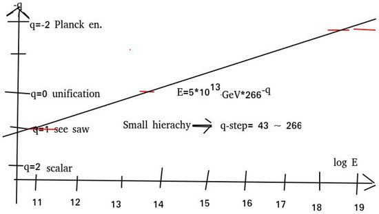
Figure 1.
The plot of the dimension-of-coefficient-related q (actually more negative q goes upwards) versus the logarithm to base 10 of the energy scale measured in GeV (we took the rather than ln, because we have given the energy scales in powers of ten, so it is easier to translate these numbers to the energy scales). We did not present the point for the “scalar” energy scale directly, because the little hierarchy mass ratios give us the ratio of the see-saw scale energy over the scalar one, and this ratio is simply the step-factor in the energy scale involved in lowering of q by one unit. The fitted value for this lowering factor, using the three scales presented, is 266. This is indeed of the order of the little hierarchy mass ratios. We successively found a chain of four quark masses, t, b, s, and u, rather close to the ratio of 43 in terms of mass (see (24a)–(24g)). This 43 deviates from 266 by less than a factor say, in as far as it is only deviating by 6.2. In the text below, we extend this plot to the scales, which require a more complicated discussion.
4.2. The More Complicated Scales
The remaining four scales were left here to the end because we consider them to be complicated in a couple of ways: The “inflaton” scale is a cosmological scale rather than a scale of physical laws, so at the end, it might not truly belong in our scheme. So far, we have only considered field theory-defined scales, but the other three scales do not have a field theory description and are rather described as single strings and single monopoles. Thus, the factor we already talked about, wherein the number of lattice hypercubes in a piece of space time varies as , is no longer relevant to these single-particle descriptions.
Finally, the “Fermion tip” scale involves very speculative extra assumptions, but to make up for that, it is associated with a reasonable fit of the density of fermion masses on the -axis.
The Inflation Scale
Thinking of the inflation rate as representing an expansion of both space and the lattice—somehow following the space expansion—it would imply a large number associated with the lattice expansion, if, during one link-length step, the world expanded faster than by of order unity. So, in the philosophy of taking the couplings of order unity at the fundamental level, we should have no faster expansion than that. But presumably, we have just that rate of expansion order of magnitude. That is to say, we expect the following:
The last point here is that we have not found any reason why a should be biased, except for the bias of being looked at in a quantum field theory in which one, in a fixed continuum region , sees a number of hypercubes proportional to . This is just the same bias as for the unification scale, and thus, we predict that the energy scale should be similar in order of magnitude to the unification scale. That is to say, we should assign to the inflation rate scale the effective q-value
We could also ask for the potential V for the inflaton field during the inflation era, or rather consider its fourth root as an energy scale. Now, however, during inflation, this V is related to the inflation rate , supposedly of order , by the FLRW equation. In fact, we have
Here, is the factor by which the scale goes up each time the q-value goes down by one unit. We found this “holy number” to be .
The value for the Hubble–Lemaitre expansion rate at the inflation time means the inflation energy scale should be of the same order as the unification scale (using approximate SU(5)). This agrees with the value of GeV obtained by Enquist [48], which is very close to that for the “unification scale”.
- LiddleAs a scale to represent the energy scale for the inflation period of the universe we may—perhaps in a bit of a biased way—choose the Hubble–Lemaitre expansion at the end of the inflation which, according to Andrew Liddle [49], takes values likeUsing the values GeV or GeV for , we obtain values for likeIn fact, the highest of these results for is only a factor 7 lower than the “unification” scale GeV, and that is not even one order of magnitude.
- EnquistIn an article by Enquist [48], we findTaking a typical (but not necessarily correct) valueEnquist’s value for H is a factor of 2 above the “unification” scale. So, we can indeed claim, as our model predicts, that the scales of unification and inflation coincide in order of magnitude. Liddle’s value for the inflation scale is below, and Enquist’s value is above the unification scale.
- Belleomo et al.In the article by Belleomo et al. [50], we findHere, r is the ratio of the tensor spectrum to the scalar one
- LiddleLiddle [49] gives a value
These scales for seems a bit too high for our argument that the highest energy density possible should be given by the lattice scale . I.e., we should have obtained the same value for in inflation as the unification scale GeV.
But it seems the fourth root of the energy density at inflation was about 200 times larger than the unification scale. However, the Hubble–Lemaitre constant at inflation seems to match our model better.
4.3. The Three Lowest Energy Scales
In order to argue for the effective q-value for the Fermion tip scale and for two other scales (namely, string and monopole), we have to first discuss how to average over the hypercubes in a fluctuating lattice in a couple of different ways.
One can indeed imagine a couple of ways of averaging:
- One way to average is simply to count all lattice hypercubes equally regardless of whether they happen to be big or small in the fluctuating lattice.
- Another method consists in analyzing their effect in what is a little finite or perhaps infinitesimal piece of space-time, because that is what will appear as the effect from a certain little region in space time. Now, if the lattice is locally dense, which means if a is small, then a higher number of hypercubes are counted in a given small region. And oppositely, when the lattice has big plaquettes, only a few hypercubes are counted in a small region. The factor by which we overcount, by asking for the contribution to a given little region, is, of course, proportional to . This factor is the same for the kinetic and the non-kinetic terms discussed for the first four “simple” scales, and thus this makes no difference to them. But this means that had we asked for an absolute value of a term in the Lagrangian, then we should use an average with included.So, when we denoted the “genuine” average link size by above, it was, in fact, an average using a weighting.
So, honestly speaking, we should define two different average link sizes
with a similar use of the Gaussian distribution, as we performed above.
So, the true maximum in the distribution of a sizes, in the sense of just counting hypercubes, is bigger than the size corresponding to the “unification scale” by a factor of = . Thinking in energy scales, the scale obtained by counting maximum number of links is times lower in energy than the unification scale.
4.3.1. The Fermion Tip Scale
This “Fermion Tip” scale is defined as an extrapolation of the density on the energy/mass axis of masses of the Fermions in the Standard Model to an energy point at which the density of Fermion masses in the Standard Model distributed on the (logarithmic) energy axis goes to zero. If we use the language of calling a fermion “active” at higher energy scales E than its mass, the tip-point we talk about is the point where all the Standard Model fermions have just become active according to a smoothed-out distribution.
The philosophy of this fermion tip scale is a somewhat complicated speculative story containing the assumption that the number of active families should, for the low-energy scales, be below the “fermion tip” point, equal to what we can call the thickness of the lattice. Really, we have in mind a tripling of the lattice so that, in reality, there should be one lattice for each family. This is what would be the case if, at higher energies, we did not simply have the Standard Model group but rather a cross-product of one Standard Model group for each family. We worked a lot on this type of model, and it is called the AntiGUT model [9,32,33,34,35,36].
To ensure the fitting of the fermion masses for the “fermion tip” scale, it is only important that
- wW extrapolate to the tip whatever distribution may fit the Standard Model masses;
- This tip point represents the maximum density of lattice hypercubes obtained by simple counting (not using field theory). It is this fact that leads to it having
We make this extrapolation to a point where the extrapolated fermion mass value density goes to zero by fitting with a formula inspired by our model in this article, the fluctuating lattice with a Gaussian distribution in the logarithm of the link size a. Really, our fitting curve for the mass value density on the logarithmic mass axis is a parabola touching the zero-density axis near the top mass. We call this point the “fermion tip” scale.
The model behind our fitting formula is based on the following physical but very speculative assumption.
Speculation for fitting: At any energy scale E below the “Fermion Tip” point, the number of “active fermions” at that scale is proportional to the number of hyper-cubes in the fluctuating lattice, with the link size corresponding to that energy ( is the correspondence). Here, “active fermions” mean fermions with a mass .
So, for example, for E larger than the top mass, all the fermions in the Standard Model are formally “active”, and the maximal amount of “active” Fermions is reached there. It follows that the density must essentially go to zero at the top mass. But now we want to replace the actual irregular density function of fermions on the energy/mass scale axis with a more smoothed-out, continuous function, and that introduces the maximal point, which we call , somewhat higher up on the mass scale.
Our next assumption for the fitting function is that the number of “inactive fermions”, as a function of the scale E, grows downward in energy E with the square of the distance in logarithm , i.e., as .
In order to see that such a fitting hypothesis is not in violent disagreement with the spectrum of Fermions, counting their numbers weighted by the number of spin and color states, we present a table made for the adjusted value of the tip-point, which is
The point is that with this value for , one can see that the quantity, which should then be constant from fermion to fermion, indeed varies very little.
In the tables below, one for the quarks and one for the charged leptons in the Standard Model, the first column gives the flavor of the particle. In column 2, we list for the group of particles with this flavor (there are three colours and two spins for each flavor, making us think of each flavor of quarks as representing 6 = 2 ∗ 3 states) the average of their numbers in mass counted from above. For example, the bunch of the six bottom quarks have numbers from 7 to 12, and the average is given as 9. The mass of the quarks is given in column 3. In the fourth column, we give the logarithm to base 10 of the mass in GeV of the bunch of fermions with the flavor named. In the next column, the fifth one, we provide the difference of this logarithm from that of our ansatz for the tip GeV, a value that we have decided on through several attempts and drawing of plots, i.e., we give minus the logarithm of the mass. The sixth column provides this difference squared, and finally, the seventh column gives this difference squared divided by the average number n in the counting from above, i.e., . If the density of mass values along the logarithm of the mass axis was indeed proceeding as a constant times , then the number should be constant (actually the constant). Indeed, the table shows that this is approximately true.
Figure 2 illustrates the type of curve to which we fit. We separated the fermions into one table for the quarks and one for the leptons just to check that both types of Standard Model fermions fit reasonably well to a parabola, as shown in Figure 2.
| Name | number n | Mass m | = | |||
| top | 3 ± 1 | 172.76 ± 0.3 GeV | 2.2374 ± 0.0008 | 1.7626 | 3.1066 ± 0.003 | 1.0355 ± 0.001 ±0.4 |
| bottom | 9 ± 0.3 | 4.18 ± 0.0079 GeV | 0.6212 ± 0.001 | 3.3788 | 11.416 ± 0.01 | 1.268 ± 0.001 ± 0.03 |
| charm | 17 or 15 | 1.27 ± 0.02 | 0.10382 ± 0.009 | 3.8962 | 15.180 ± 0.07 | 0.893 ± 0.004 ± 0.06 |
| strange | 25 or 23 | 0.095 ± 0.006 GeV | −1.0223 ± 0.003 | 5.0223 | 25.223 ± 0.03 | 1.009 ± 0.001 ± 0.1 |
| down | 31 | 4.79 ± 0.16 MeV | −2.3197 ± 0.01 | 6.3197 | 39.939 ± 0.06 | 1.288 ± 0.002 |
| up | 37 | 2.01 ± 0.14 MeV | −2.6968 ± 0.03 | 6.6968 | 44.847 ± 0.4 | 1.212 ± 0.01 |
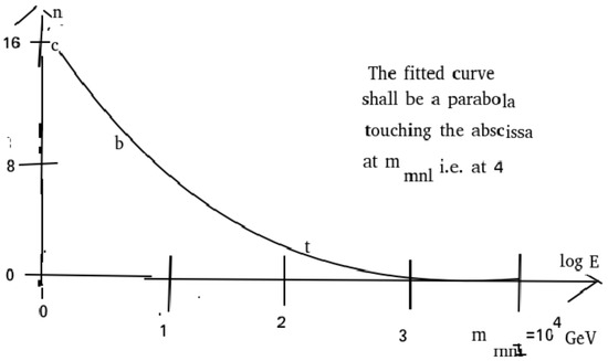
Figure 2.
Because the distribution of the log of the link size has a maximum at the fermion tip point, we suggest that the density of active fermions (=fermions with a lower mass than the scale E, at which you ask for the density of links) should behave this way, meaning with a parabolic behaviour and a maximum at the point (=the fermion tip point). If we take it that there are 15 chiral fermions per family, the number of families at chiral fermion number n counted from the top downwards in mass will be “Number of active families” = (3 * 15 − n)/15. It is important to note that the three labeled points, c, b, and t, fit better on the parabola than on a straight line. So, the chosen fitting form has some empirical support.
| Name | number n | Mass m | = | |||
| 13 or 19 | 1.77686 ± 0.00012 | 0.2496 ± 0.00003 | 3.7503 | 14.065 ± 0.0003 | 1.082 ± 0.00002 ±0.4 | |
| mu | 21 or 27 | 105.6583745 ± MeV | 4.9761 | 24.761 ± | 1.179 ± ± 0.3 | |
| electron | 41 | 0.51099895069 ± | −3.2915 ± | 7.2916 | 53.167 ± | 1.297 ± |
Our fitting of the fermion mass spectrum is based on a philosophy that below the energy scale , we assume a density of “active” (meaning effectively massless at the relevant scale ) fermion components (where is the number in the mass series counted from high mass at the running scale ) that satisfies the proportionality
with the notation of the tables.
So
We would have expected, in our philosophy, that this spread from the fermion distribution should have been the same as the spread from the distribution of the scales, which is our main interest in this article. But they seem to deviate by about a factor of 2. This is, of course, embarrassingly large, since the and are already logarithms, and the approximate equality should be more accurate than that. However, the point GeV at which we obtain the successful fit of the masses of the quarks and leptons is essentially an extrapolation toward the high-mass part of the spectrum and should be determined well, even if we do not obtain theoretical success with .
4.3.2. The Monopole Scale
It is well-known [51] that in lattice gauge theories, one obtains monopoles if it is possible, i.e., if the fundamental group is non-trivial, as in the Standard Model group [7,8,52] , where it is . The Standard Model group in the O’Raifeartaigh [52] sense is the group with the Lie algebra of the Standard Model , but with its global structure arranged so that the representations of the group automatically obey the quantization rules of electric charge being an integer for colorless particles and having the right charge known for the colored particles, the quarks. The group achieving that is the group , which consists of 5 by 5 matrices with the matrices for and along the diagonal and the determinant of the full 5 by 5 matrix restricted to unity.
On the lattice with link variables taking values in the Standard Model group, one will now expect Dirac strings and monopoles associated with the elements in , which means closed non-contractable loops inside this group. So, there should be different types of monopole corresponding to such loops inside the group. Those with the smallest abelian monopole charge have both weak and color-magnetic charge. So, we might expect that the easiest combinations to form would be pairs of monopoles confined much like quark anti-quark pairs, but now with a color magnetic binding instead of color-electric fields connecting them.
In whatever form they should be found, and the order of magnitude of their mass should be estimated by thinking of the track of a monopole as a series of cubes in the lattice, with each of the six plaquette sides carrying approximately 1/6 of the monopole charge. Each such cube in the series would have a cost of order unity in the action. So, the action for a such a long chain of monopolic cubes, or simply a long time track for a monopole, contributes to the action term of the order of the length of the chain measured in link-lengths. A similar time track in the continuum limit is of the order , where is the infinitesimal distance element along the time track, and m is the mass of the particle, here the monopole. So, we identify
where a is the link size of the lattice used. This, of course, gives us—what must be true from dimensional arguments anyway—that
where it is easily seen that the averaging should be taken in the pure counting sense, since we did not use any field theory here. This means an effective q to obtain the average must be
This suggests, from our straight-line fit, an energy scale of the order 40 GeV or 38 GeV. eEtremely small deviations from the Standard Model have been seen at LHC, but in fact, there was one possible statistical fluctuation, giving a dimuon resonance with mass GeV and width GeV [29]. The statistical significance globally is 3.0 s.d.
In addition, Arno Heister [53] found, by analyzing old ALEPH data, an enhancement at 30 GeV in mass for a dimuon.
We may take these uncertain observations as suggesting a monopole scale at
4.3.3. The String Scale
Let us suppose that there was a string theory scale, and we know the usual Nambu–Goto action being of the form
where the integral over the area measure means the area of the time track of the string. The coefficient is in a partly historical notation
where is the Regge pole slope used in the Veneziano model.
It is not surprising that an area of proportional action should be proportional to the lattice link length squared, as is also enforced by the dimensionality of the coefficient
Thus, the effective q for the string scale, if there were one, would be
With an immediate estimate using, say, a factor of 250 or 266 in the energy scale for each step in q, we find that the string energy scale should be
This suggests very strongly that we should take the appearance of string-like physics in hadron physics as giving us a string scale. We can say the following:
4.3.4. Fit of the Low-Energy Scales
In the fluctuating lattice model, three of our energy scales have their average obtained via the simple counting hypercubes way (rather than the method we used for the field theory-related scales). So here, we present a straight line fit for these three alone (Figure 3).
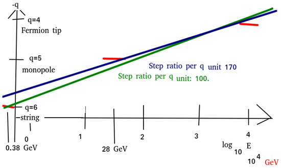
Figure 3.
Here we present a sub-figure of our full fit of all the energy scales to include only the “fermion tip” scale and the two scales, which we imagine being described by an action for a single object, the monopole particle or the string, developping through space time. We see that these three scales by themselves lie on a straingt line as our model predicts, although the best fit to the value of B in the fitting formula for the energy of the energy scales for these three is rather than the for everyhting.
4.4. Total Fit Line
Finally, we present a straight line fit for all eight energy scales (Figure 4).
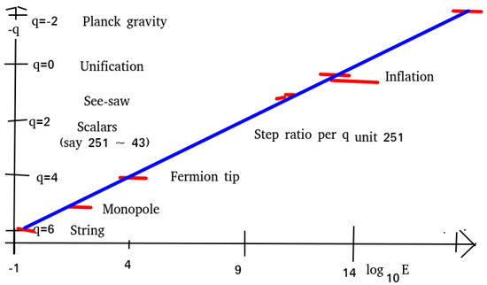
Figure 4.
Here the looking for if all the energy scales enegies (logaritmically) lies on straight line versus q as we predict. Indeed they fit well a straight line of the form with as written . The susy-point, which would not have fitted so well, was left out, since in this article reader should take it, that we do not believe in susy. The energy scale “scalars” was replaced by a statement, because the experimental numbers from the mass ratios of various fermions in the Standard Model are not related directly to the “scalars” scale, but rather to the ratio of this scale to the “see-saw” scale, thus giving the slope parameter B, but not the energy scale itself. The bracket “” should mean that the number 43 for the typical fermion mass ratio is not so far from the . Note that ordinate axes on our figures are denoted , and that the abscissa is the logarithm of the energy scale, using 10 as basis to make the relation with the energy numbers easy to see.
5. Fluctuating Gauge Argument for Fluctuating Lattice
In the article “Dynamical Stability…Light, written by Chaos”, Førster, Ninomiya, and myself [25,54], it is suggested that gauge theories could appear with exact gauge symmetry, even if fundamentally there was only approximate symmetry. The reason for this is that very strong quantum fluctuations occur in the gauge, even if the gauge symmetry is weakly broken in the fundamental action. In this way, the final small breaking is washed out. It is important to note that, with our philosophy, there exists an a priori fundamental variable corresponding to the gauge degree of freedom, although it might be interpreted differently in practice. But there is an ontologically existing depth of field for that. For the gravity case, M. Lehto et al. [55] argued for deriving translational invariance in this spirit. If this is the mechanism for obtaining the gauge symmetry of reparametrization in gravity, then the coordinate system will fluctuate strongly. Here, we take the point of view that some gauge degrees of freedom exist in nature, and they are ontological. Now, such fluctuations in the coordinates are supposed to carry a lattice with them, and we, who work with a coordinate system that is specified by some conditions, think of a coordinate system very differently from the ontological one. We suppose that the ontological coordinate system and the associated lattice fluctuate wildly. That is to say, a model for obtaining gauge symmetries via quantum fluctuations actually effectively leads to a fluctuating lattice.
In the first approximation, our fluctuating lattice behaves just as it should with such a philosophy for how gauge symmetry comes about. However, if it were taken completely seriously, then the lattice should fluctuate into a superposition with some components deviating divergently from others. In our fit, we have a convergent fluctuation in the link scale, but it is large in the sense that it gives rise to large numbers, with our step ratio per q unit of 251.
Somehow, there is a need for making the fluctuations of the lattice limited, instead of the a priori infinite-scale fluctuations that would correspond to perfect reparametrization symmetry.
I would say that having a large number (such as our 251), in the place where it should a priori have been infinite, is somewhat nice.
6. Conclusions
We have in this article connected a series of energy scales found in physics—and strictly speaking expected to be equal to “the fundamental energy scale”. But the eight scales we considered deviate significantly, even in order of magnitude. This is philosophically somewhat unexpected. The present article has repaired that problem by proposing that a fundamentally existing fluctuating lattice could unite these eight energy scales as all coming from the same fluctuating lattice. They are thus all deduced from the distribution of the link size for the fluctuating lattice. In our simple Gaussian in the logarithm ansatz, this means that the eight energy scales are given by—and fitted by—just two parameters, the overall scale and the width of the assumed Gaussian distribution. This width is dimensionless and takes the value . Instead of the width, we might represent the parameter for which so many energy scales can be fitted as the step factor and by which the energy scale goes up each time a quantity q, related to the dimensionality of the coefficients of the actions involved at the various energy scales, is lowered by one unit. Then, one could say that the “holy parameter”, the step factor, is about 251.
If one would take the scales with large q-values seriously, then at least some of the fundamental scales are in the region where present-day and future experiments have a chance to find, e.g., non-locality or other effects of the lattice. This gives much more promising prospects for investigating fundamental physics experimentally in the not-so-distant future, than if—as I believed myself until recently—the Planck scale was the fundamental scale for physics.
With this work, we would rather consider, for example, the “fermion tip scale” as the most fundamental one. The fermion tip scale is already formally reached by LHC, although to really confirm whether or not there were, say, non-local effects at GeV might, in practice, require somewhat higher-energy accelerators.
6.1. Failures
At the end, we still admit that, although we invented a “scalars” scale where there should exist a lot of scalar bosons, the Standard Model Higgs scalar boson has such a fine-tuned mass that it does not at all fit into the “scalars scale”. Personally, I would expect that, in order to obtain a sufficiently fine-tuned Higgs mass, something like our complex action theory, in which fine-tunings can be modeled and can even depend on the future [56,57,58,59,60,61,62,63,64,65,66,67,68,69,70], is needed.
Similarly, one might have hoped to obtain the value of the cosmological constant via a formalism analogous to the string theory, giving the hadron string scale and the monopole scale. One should, by understanding the cosmological constant as the action density for a space filling three-brane, expect the value to deliver the scale of the cosmological constant; however
Here, we used the vacuum energy density, or the approximate critical energy density , see, e.g., [71]. The two values GeV and GeV are not even close in order of magnitude. So, the cosmological constant provides another failure for our model and must somehow be fine-tuned (with fine-tuning completely spoiling our prediction in the present article)! Personally, I would say that fine-tuning has overwritten our order of magnitude model [72], in which we give an argument for a zero cosmological constant in the complex action and influence from future spirit.
6.2. Yet a Possible Scale?
However, looking similarly for domain walls or two-branes, we would obtain the predicted scale . This is not far from the energy scale used for the tension in the domain walls fitted to Colin Froggatt’s model and my dark matter model, in which we have a scale of the order of a few MeV (the wall tension we fitted was [73]).
Funding
This research received no external funding.
Data Availability Statement
No new data were created or analyzed in this study. Data sharing is not applicable to this article.
Acknowledgments
The author thanks the Niels Bohr Institute for his status as emeritus. This work was discussed in both the Bled Workshop and the Corfu Institute in 2024. He also thanks Colin D. Froggatt, Glasgow University, for having significantly improved the English of the article.
Conflicts of Interest
The author declares no conflicts of interest.
References
- Nielsen, H.B. Approximate SU(5), Fine structure constants. Universe 2025, 11, 32. [Google Scholar] [CrossRef]
- Howard, G.; Sheldon, G. Unity of All Elementary-Particle Forces. Phys. Rev. Lett. 1974, 32, 438. [Google Scholar] [CrossRef]
- Masiero, A.; Nanopoulos, A.; Tamvakis, K.; Yanagida, T. Naturally Massless Higgs Doublets in Supersymmetric SU(5). Phys. Lett. B 1982, 115, 380–384. [Google Scholar] [CrossRef]
- Laperashvili, L.; Ryzhikh, D. [SU(5)]3 SUSY unification. arXiv 2001, arXiv:hep-th/0112142. [Google Scholar]
- Senjanovic, G.; Zantedeschi, M. Minimal SU(5) theory on the edge: The importance of being effective. arXiv 2024, arXiv:2402.19224v1. [Google Scholar] [CrossRef]
- Nielsen, H.B.; Bennett, D. Seeking a Game in which the standard model Group shall Win. Bled Work. Phys. 2011, 12, 149. [Google Scholar]
- Nielsen, H.B. Small Representations Explaining, Why standard model group? PoS CORFU 2015, 2014, 045. [Google Scholar]
- Nielsen, H. Dimension Four Wins the Same Game as the Standard Model Group. Phys. Rev. D 2013, 88, 096001. [Google Scholar] [CrossRef]
- Nielsen, H.B. Random Dynamics and relations between the number of fermion generations and the fine structure constants. Acta Phys. Pol. Ser. B 1989, 20, 427. [Google Scholar]
- Cea, P.; Cosmai, L. Deconfinement phase transitions in external fields. In Proceedings of the XXIIIrd International Symposium on Lattice Field Theory, Trinity College, Dublin, Ireland, 25–30 July 2005. [Google Scholar]
- Laperashvili, L.V.; Ryzhikh, D.A.; Nielsen, H.B. Phase transition couplings in U(1) and SU(N) regularized gauge theories. Int. J. Mod. Phys. A 2001, 16, 3989–4009. [Google Scholar] [CrossRef]
- Laperashvili, L.V.; Nielsen, H.B.; Ryzhikh, D.A. Phase transition in gauge theories and multiple-point model. Phys. Atom. Nuclei 2002, 65, 353–364. [Google Scholar] [CrossRef]
- Das, C.R.; Froggatt, C.D.; Laperashvili, L.V.; Nielsen, H.B. Flipped SU(5), see-saw scale physics and degenerate vacua. arXiv 2005, arXiv:hep-ph/0507182. [Google Scholar]
- Nielsen, H.B.; Kleppe, A. Bled Workshop July 2019, “What comes Beyand the Standard Models”. Available online: http://bsm.fmf.uni-lj.si/bled2019bsm/talks/HolgerTransparencesconfusion2.pdf (accessed on 31 March 2025).
- Bennett, D.L.; Nielsen, H.B.; Brene, N.; Mizrachi, L. The Confusion Mechanism and the Heterotic String. In Proceedings of the 20th International Symposium on the Theory of Elementary Particles, Ahrenshoop, Germany, 13–17 October 1986. [Google Scholar]
- Minkowski, P. μ→eγ at a rate of one out of 109 muon decays? Phys. Lett. B 1977, 67, 421–428. [Google Scholar] [CrossRef]
- Mohapatra, R.N.; Senjanovic, G. Neutrino Mass and Spontaneous Parity Nonconservation. Phys. Rev. Lett. 1980, 44, 912. [Google Scholar] [CrossRef]
- Funkhouser, S. The fundamental scales of structures from first principles. arXiv 2008, arXiv:0804.2443. [Google Scholar]
- Stojkovic, D. Can We Push the Fundamental Planck Scale Above 1019 GeV? Available online: https://cds.cern.ch (accessed on 31 March 2025).
- Vergeles, S.N. Wilson fermion doubling phenomenon on irregular lattice: The similarity and difference with the case of regular lattice. arXiv 2015, arXiv:1502.03349v2. [Google Scholar] [CrossRef]
- Brockmann, R.; Frank, J. Lattice quantum hadrodynamics. Phys. Rev. Lett. 1992, 68, 1830. [Google Scholar] [CrossRef]
- Lüscher, M. Advanced Lattice QCD Desy 98-017 August 2006 (Lectures). Available online: https://luscher.web.cern.ch/luscher/lectures/LesHouches97.pdf (accessed on 31 March 2025).
- Wagner, A.J.; Strand, K. Fluctuating lattice Boltzmann method for the diffusion equation. Phys. Rev. E 2016, 94, 033302. [Google Scholar] [CrossRef][Green Version]
- Froggatt, C.D.; Nielsen, H.B. Hierarchy of quark masses, cabibbo angles and CP violation. Nucl. Phys. B 1979, 147, 277–298. [Google Scholar] [CrossRef]
- Foerster, D.; Nielsen, H.B.; Ninomiya, M. Dynamical stability of local gauge symmetry Creation of light from chaos. Phys. Lett. B 1980, 94, 135–140. [Google Scholar] [CrossRef]
- Kalecki, M. On the Gibrat Distribution. Econometrica 1945, 13, 161–170. [Google Scholar] [CrossRef]
- Pestieau, P.; Possen, U.M. A model of income distribtuion. Eur. Econ. Rev. 1982, 17, 279–294. [Google Scholar] [CrossRef]
- Johnson, N.L.; Kotz, S.; Balakrishnan, N. “14: Lognormal Distributions”, Continuous univariate distributions. In Wiley Series in Probability and Mathematical Statistics: Applied Probability and Statistics, 2nd ed.; John Wiley & Sons: New York, NY, USA, 1994; Volume 1, ISBN 978-0-471-58495-7. [Google Scholar]
- The CMS Collaboration. Search for resonances in the mass spectrum of muon pairs produced in association with b quark jets in proton-proton collisions at s = 8 and 13 TeV. arXiv 2018, arXiv:1808.01890v2.
- Volovik, G.E. Introduction: Gut and Anti-Gut; Oxford University Press: Oxford, UK, 2009; pp. 1–8. [Google Scholar] [CrossRef]
- Picek, I. Critical Couplings And Three Generations in a Random-Dynamics Inspired Model. Fizika B 1992, 1, 99–110. [Google Scholar]
- Bennett, D.; Nielsen, H.B.; Picek, I. Understanding fine structure constants and three generations. Phys. Lett. B 1988, 208, 275–280. [Google Scholar] [CrossRef]
- Nielsen, H.B.; Brene, N. Gauge Glass. In Proceedings of the XVIII International Symposium on the Theory of Elementary Particles, Ahrenshoop, Germany, 21–26 October 1984. [Google Scholar]
- Bennett, D.L.; Brene, N.; Mizrachi, L.; Nielsen, H.B. Confusing the heterotic string. Phys. Lett. B 1986, 178, 179–186. [Google Scholar] [CrossRef]
- Bennett, D.L.; Nielsen, H.B. Predictions for Nonabelian Fine Structure Constants from Multicriticality. arXiv 1993, arXiv:hep-ph/9311321v1. [Google Scholar]
- Bennett, D.L.; Nielsen, H.B. Gauge Couplings Calculated from Multiple Point Criticality Yield α−1 = 137 ± 9: At Last, the Elusive Case of U(1). arXiv 1996, arXiv:hep-ph/9607278. [Google Scholar] [CrossRef]
- Thoren, J. Grand Unified Theories: SU (5), SO(10) and Supersymmetric SU (5). Bachelor’s Thesis, Lund University, Lund, Sweden, 2012. [Google Scholar]
- Nielsen, H.B.; Takanishi, Y. Baryogenesis via lepton number violation in Anti-GUT model. arXiv 2001, arXiv:hep-ph/0101307. [Google Scholar] [CrossRef]
- Froggatt, C.D.; Nielsen, H.B.; Takanishi, Y. Family replicated gauge groups and large mixing angle solar neutrino solution. Nucl. Phys. B 2002, 631, 285. [Google Scholar] [CrossRef][Green Version]
- Nielsen, H.B.; Takanishi, Y. Five adjustable parameter fit of quark and lepton masses and mixings. Phys. Lett. B 2002, 543, 249. [Google Scholar] [CrossRef][Green Version]
- King, S.F. Neutrino Mass and Mixing in the Seesaw Playground. Nucl. Phys. B 2016, 908, 456–466. [Google Scholar] [CrossRef]
- Mohapatra, R.N. Physics of Neutrino Mass. In Proceedings of the SLAC Summer Institute on Particle Physics (SSI04), Menlo Park, CA, USA, 2–13 August 2004. [Google Scholar]
- Grimus, W.; Lavoura, L. A neutrino mass matrix with seesaw mechanism and two-loop mass splitting. arXiv 2000, arXiv:hep-ph/0007011v1. [Google Scholar] [CrossRef]
- Davidson, S.; Ibarra, A. A lower bound on the right-handed neutrino mass from leptogenesis. arXiv 2002, arXiv:hep-ph/0202239v2. [Google Scholar] [CrossRef]
- Nielsen, H.B.; Froggatt, C.D. Masses and mixing angles and going beyond the Standard Model. arXiv 1999, arXiv:hep-ph/9905445. [Google Scholar]
- Nielsen, H.B.; Takanishi, Y. Neutrino mass matrix in Anti-GUT with see-saw mechanism. Nucl. Phys. B 2001, 604, 405. [Google Scholar] [CrossRef][Green Version]
- Feruglio, F. Fermion masses, critical behavior and universality. arXiv 2023, arXiv:2302.11580. [Google Scholar] [CrossRef]
- Enquist, K. Cosmologicaæ Infaltion. arXiv 2012, arXiv:1201.6164v1. [Google Scholar]
- Liddle, A. An Introduction to Cosmological Inflation. arXiv 1999, arXiv:astro-ph/9901124v1. [Google Scholar]
- Bellomo, N.; Bartolo, N.; Jimenez, R.; Matarrese, S.; Verde, L. Measuring the Energy Scale of Inflation with Large Scale Structures. arXiv 2018, arXiv:1809.07113v2. [Google Scholar] [CrossRef]
- Auzzi, R.; Bolognesi, S.; Evslin, J.; Konishi, K.; Murayama, H. Nonabelian Monopoles. arXiv 2004, arXiv:hep-th/0405070v3. [Google Scholar]
- O’Raifeartaigh, L. The Dawning of Gauge Theory; Princeton University Press: Princeton, NJ, USA, 1997. [Google Scholar]
- Heister, A. Observation of an excess at 30 GeV in the opposite sign di-muon spectra of Z → bb + X events recorded by the ALEPH experiment at LEP. arXiv 2016, arXiv:1610.06536v1. [Google Scholar]
- Nielsen, H.B. Field theories without fundamental gauge symmetries. Philos. Trans. R. Soc. Lond. Ser. A Math. Phys. Sci. 1983, 310, 261–272. [Google Scholar] [CrossRef]
- Lehto, M.; Nielsen, H.B.; Ninomiya, M. Time translational symmetry. Phys. Lett. B 1989, 219, 87–91. [Google Scholar] [CrossRef]
- Nagao, K.; Nielsen, H.B. Automatic Hermiticity. Prog. Theor. Phys. 2011, 125, 633. [Google Scholar] [CrossRef][Green Version]
- Nielsen, H.B. Complex Action Support from Coincidences of Couplings. arXiv 2011, arXiv:1103.3812v2. [Google Scholar] [CrossRef]
- Nielsen, H.B. Remarkable Relation from Minimal Imaginary Action Model. arXiv 2011, arXiv:1006.2455v2. [Google Scholar]
- Nagao, K.; Nielsen, H.B. Formulation of Complex Action Theory. arXiv 2012, arXiv:1104.3381v5. [Google Scholar] [CrossRef]
- Nielsen, H.B.; Ninomiya, M. Intrinsic periodicity of time and nonmaximal entropy of universe. Int. J. Mod. Phys. A 2006, 21, 5151. [Google Scholar] [CrossRef]
- Bennett, D.L. Multiple Point Criticality, Nonlocality, and Finetuning in fundamental physics: Predictions for Gauge Coupling Constants gives α−1 = 136.8 ± 9. arXiv 1996, arXiv:hep-ph/9607341. [Google Scholar]
- Nielsen, H.B.; Ninomiya, M. The proceedings of Bled 2006—What Comes Beyond the Standard Models. arXiv 2006, arXiv:hep-ph/0612250. [Google Scholar]
- Nielsen, H.B.; Ninomiya, M. Test of Influence from Future in Large Hadron Collider: A Proposal. Int. J. Mod. Phys. A 2009, 24, 3945–3968. [Google Scholar] [CrossRef]
- Nielsen, H.B.; Ninomiya, M. Search for effect of influence from future in large hadron collider. Int. J. Mod. Phys. A 2008, 23, 919. [Google Scholar] [CrossRef]
- Nielsen, H.B.; Ninomiya, M. Unification of cosmology and second law of thermodynamics: Solving cosmological constant problem, and inflation. Prog. Theor. Phys. 2007, 116, 851. [Google Scholar] [CrossRef]
- Nielsen, H.B.; Ninomiya, M. The proceedings of Bled 2007—What Comes Beyond the Standard Models. arXiv 2007, arXiv:hep-ph/0711.4681. [Google Scholar]
- Nielsen, H.B.; Ninomiya, M. Card game restriction in LHC can only be successful! arXiv 2009, arXiv:0910.0359. [Google Scholar]
- Nielsen, H.B.; Ninomiya, M. Degenerate vacua from unification of second law of thermodynamics with other laws. arXiv 2007, arXiv:hep-th/0701018. [Google Scholar]
- Nielsen, H.B. Initial Condition Model from Imaginary Part of Action and the Information Loss. arXiv 2009, arXiv:0911.3859. [Google Scholar]
- Nielsen, H.B.; Borstnik, M.S.M.; Nagao, K.; Moultaka, G. The proceedings of Bled 2010—What Comes Beyond the Standard Models. arXiv 2010, arXiv:hep-ph/1012.0224. [Google Scholar]
- Solà, J. Cosmological constant and vacuum energy: Old and new ideas. J. Phys. Conf. Ser. 2013, 453, 012015. [Google Scholar] [CrossRef]
- Nielsen, H.B. String Invention, Viable 3-3-1 Model, Dark Matter Black Holes. arXiv 2024, arXiv:2409.13776. [Google Scholar] [CrossRef] [PubMed]
- Froggatt, C.D.; Nielsen, H.B. Domain Walls and Hubble Constant Tension. arXiv 2024, arXiv:2406.07740. [Google Scholar]


Disclaimer/Publisher’s Note: The statements, opinions and data contained in all publications are solely those of the individual author(s) and contributor(s) and not of MDPI and/or the editor(s). MDPI and/or the editor(s) disclaim responsibility for any injury to people or property resulting from any ideas, methods, instructions or products referred to in the content. |
© 2025 by the author. Licensee MDPI, Basel, Switzerland. This article is an open access article distributed under the terms and conditions of the Creative Commons Attribution (CC BY) license (https://creativecommons.org/licenses/by/4.0/).