Abstract
Phase stability at low radio frequencies is severely impacted by ionospheric propagation delays. Radio interferometers such as the giant metrewave radio telescope (GMRT) are capable of detecting changes in the ionosphere’s total electron content (TEC) over larger spatial scales and with greater sensitivity compared to conventional tools like the global navigation satellite system (GNSS). Thanks to its unique design, featuring both a dense central array and long outer arms, and its strategic location, the GMRT is particularly well-suited for studying the sensitive ionospheric region located between the northern peak of the equatorial ionization anomaly (EIA) and the magnetic equator. In this study, we observe the bright flux calibrator 3C48 for ten hours to characterize and study the low-latitude ionosphere with the upgraded GMRT (uGMRT). We outline the methods used for wideband data reduction and processing to accurately measure differential TEC () between antenna pairs, achieving a precision of< mTECU (1 mTECU = TECU) for central square antennas and approximately mTECU for arm antennas. The measured values are used to estimate the TEC gradient across GMRT arm antennas. We measure the ionospheric phase structure function and find a power-law slope of , indicating deviations from pure Kolmogorov turbulence. The inferred diffractive scale, the spatial separation over which the phase variance reaches , is ∼6.66 km. The small diffractive scale implies high phase variability across the field of view and reduced temporal coherence, which poses challenges for calibration and imaging.
1. Introduction
The ionosphere remains a persistent barrier to radio frequency observations from the ground, with its impact being especially significant in high-resolution interferometric imaging. This highly variable, partially ionized plasma medium introduces several propagation effects, such as refraction, dispersion, group delay, and Faraday rotation [1,2]. Major interferometers like the giant metrewave radio telescope (GMRT)1, the very large array (VLA)2, the low-frequency array (LOFAR)3, and the Murchison wide-field array (MWA)4, as well as the upcoming square kilometre array (SKA) [3], are all susceptible to ionospheric disturbances. Although advances in low-frequency radio instrumentation now allow us to investigate ionospheric properties with unprecedented sensitivity and resolution, compensating for ionospheric-induced errors in observational data remains a persistent challenge, particularly for long baselines and low frequencies below 1 GHz.
The ionosphere’s behavior varies spatially and temporally, influenced by solar radiation, geomagnetic activity, which is maximum around the geomagnetic equator [4], and atmospheric conditions. During the daytime, enhanced ionization leads to stronger propagation effects, whereas at night, the ionosphere becomes more stable; however, it may still add phase errors [1] to incoming radio waves. Rapid fluctuations in the total electron content (TEC) can cause signal deflection, scintillation, and differential delays between antennas in an array, which severely affect the coherence of astronomical signals [5,6]. For precision imaging, especially at frequencies below a few hundred megahertz, accurate modeling and correction of these ionospheric perturbations are essential.
Interferometric arrays such as the VLA (located at approximately N) have been employed to investigate small-scale ionospheric fluctuations on the order of 0.1 million total electron content units () by observing a single bright source within the field of view (FoV) [7,8]. These studies analyze the ionosphere’s behavior through Fourier analysis of phase measurements from individual antennas. In contrast, wide-field interferometers, capable of detecting multiple celestial radio sources simultaneously, utilize positional offsets to probe ionospheric structures [9,10]. Additionally, Helmboldt et al. [11] identified groups of wave-like disturbances by performing spectral analysis on the position shifts of 29 bright sources within a single FoV observed by the VLA. Using LOFAR (located at mid-latitude), Mevius et al. [12] found that ionospheric irregularities (TEC) were anisotropic at night with an accuracy of total electron content (TEC).
The ionosphere behaves as a cold, collision-less plasma, and its refractive index n varies with both the position and time of the observation, making the problem more complex. At frequencies well above the ionosphere’s plasma frequency (∼1–10 MHz), the refractive index can be expanded using a Taylor series approximation (see, e.g., [1,13]. In this regime, the dominant term in the expansion corresponds to a dispersive phase delay proportional to the total electron content (TEC) along the line of sight. The resulting ionospheric phase shift can be expressed as follows:
where is the electron density along the path, e is the elementary charge or electronic charge, is the electron mass, c is the speed of light, and is the permittivity of free space. The total electron content (TEC) is defined as the integral of the electron number density along the path s of a signal through the ionosphere:
where is measured in , and the TEC is typically expressed in TEC units (TECU), with .
Neglecting higher-order terms in the Taylor series of the refractive index [13], the first-order additional phase shift due to the ionosphere can be conveniently expressed as follows:
where is the observing frequency in Hz, and TEC refers to the line of sight integrated electron density in units of TECU.
The study of the Earth’s ionosphere using radio interferometers has traditionally been constrained by the geographic locations of the telescopes, limiting observations to the local ionospheric regions directly above the arrays. In this context, the giant metrewave radio telescope (GMRT) offers a distinct advantage because of its favourable geographic location. Located at a latitude of 05′35.2″ N and longitude of 03′01.7″ E, the GMRT lies in a geophysically sensitive region between the magnetic equator and the northern crest of the equatorial ionization anomaly (EIA), an important feature of the low-latitude ionosphere [13]. Ionospheric activity in the EIA regions can also disrupt the operation of the global positioning system (GPS). The activation of the equatorial ionization anomaly (EIA) in the evening is mainly caused by a process called pre-reversal enhancement. This happens around sunset when changes in the electric field and ionospheric dynamics strengthen the upward movement of plasma near the equator. As a result, the two bands (or “crests”) of high electron density on either side of the magnetic equator become more pronounced. This evening increase in EIA strength is a key factor in the formation of plasma bubbles and other ionospheric disturbances [14]. Mangla and Datta [15] recently used the GMRT to observe the quasar 3C68.2 during a quiet period of solar activity. They found stronger ionospheric fluctuations than those seen with other telescopes like the VLA, LOFAR, and MWA. This was expected because the GMRT is located near the magnetic equator, where the ionosphere is usually more active.
In this study, we focus on closely examining the ionospheric information captured during a single ten-hour observation using the upgraded giant metrewave radio telescope (uGMRT, Gupta et al. [16]), which is an enhanced version of the original GMRT with improved receivers, wider frequency coverage, and advanced backend systems. The entire observation was carried using the Band-4 of uGMRT, which operates in a 550–750 MHz frequency range. The observation targets one of the brightest flux calibrators in the sky, 3C48. The 3C48 is a bright extra-galactic quasar commonly used for flux density and bandpass calibration in radio astronomy due to its compactness and high brightness (e.g., Perley and Butler [17]). Its steady flux density across radio frequencies makes it a reliable calibrator for ionospheric studies. After the data were flagged and averaged, they were calibrated using the common astronomy software application (CASA) software package [18], which is a widely used software suite for processing and analyzing radio astronomical data, particularly from interferometric arrays. During the calibration process, we estimated the complex bandpass gains by adjusting them to minimize the difference between the observed visibilities and those predicted by the model. The resulting calibration gains captured all distortions that occurred between the source and the antenna, including unmodeled variations in the antenna gain pattern, instrument-related errors, and ionospheric effects [19]. This study provides a valuable opportunity to develop and refine techniques for future data processing procedures, enhance our understanding of the physical processes driving the observed behavior, and mitigate major ionospheric-induced systematic effects in uGMRT data. Although multiple global positioning system (GPS) stations located near the Murchison Radio-Astronomy Observatory are marginally used to calibrate interferometric observations [20], there are very few GNSS stations available around the GMRT site. The closest known GNSS station is located in Hyderabad, approximately 500 km from the GMRT, making it challenging to characterize fine-scale ionospheric variability. The work presented here represents one of the first systematic investigations of the Earth’s ionosphere conducted using the wide-band receiver of the upgraded GMRT.
The structure of this paper is organized as follows. In Section 2, we describe the uGMRT observations and data processing, including radio frequency interference (RFI) mitigation, calibration steps, and phase corrections. Section 3 outlines the methodology for extracting ionospheric information, including estimates of and gradients from the calibrated phases. Finally, in Section 4, we present our discussions and the future outlook of this paper.
2. Observation and Processing
The GMRT (giant metrewave radio telescope) is one of the most sensitive and fully operational radio telescopes designed for low-frequency observations [21]. It comprises 30 parabolic dishes, with a diameter of 45 m, spread across a 25 km region. This configuration provides a total collecting area of around 30,000 at meter wavelengths, which is crucial for sensitive, high-resolution (a few arc-seconds) imaging.
Of the 30 antennas, 14 are positioned randomly within a central square measuring approximately , while the remaining 16 are distributed along three arms extending about 14 km each in a roughly ‘Y’-shaped formation. This layout allows for the study of ionospheric variations over a broad spectrum of spatial scales, as discussed in [5]. The GMRT’s location (latitude: N, longitude: E) places it in a geophysically significant area between the magnetic equator and the northern crest of the EIA [13], making it an excellent instrument for ionospheric studies. Similar to the very large array (VLA), the GMRT’s ‘Y’-shaped configuration enables observations of ionospheric fluctuations in three distinct directions, further enhancing its capability to explore ionospheric dynamics.
We proposed uGMRT observations of 3C48 at Band-4 for 10 h (proposal code: 47_0035), approximately close to the meridian transit of the source. The 3C48 is a bright, compact quasar with a flux density of approximately 5.7 Jy at 4.8 GHz [22]. The bright quasar 3C48 (J2000: RA 01 h 37 m 41 s, DEC + 33 d 09 m 35 s) was chosen as it dominates the visibilities and enables reliable ionospheric characterization.
We focus exclusively on night-time ionospheric conditions. Since 3C48 is only observable at night during winter, observations were conducted in November 2024. The dataset covers a total bandwidth of 200 MHz, ranging from 550 MHz to 750 MHz. The integration time for data recording was 2.68 s. The full bandwidth was divided into 8192 channels, with a channel resolution of 24.41 kHz. More details about the observations are summarized in Table 1. For ease of computation, in this study, we used data from 3908 channels. Each channel had a bandwidth of 24.4 kHz, spanning frequencies from 553 MHz to 648 MHz, with a central frequency of approximately 600 MHz.

Table 1.
Observation summary.
2.1. RFI Mitigation
Radio frequency interference (RFI) degrades the sensitivity of radio observations by increasing system noise and distorting calibration solutions. It also restricts the usable frequency bandwidth, with particularly severe effects at sub-GHz frequencies in GMRT data.
To mitigate RFI, we first remove strong interference and then apply an automated flagging algorithm using the TFCROP task from the common astronomy software applications (CASA) package [18]. This algorithm identifies outliers in the 2D time-frequency space for each baseline. It operates iteratively, using a user-defined sliding time window to establish a clean band-shape template that excludes RFI-contaminated regions.
During each iteration, the algorithm calculates the standard deviation between the data and the fitted template, flagging points that exceed a set threshold: 4-sigma in the time domain and 3-sigma in the frequency domain, which is optimized for strong narrow-band RFI. Additionally, we enable the EXTEND mode in CASA to flag data when TFCROP identifies RFI in at least of the time-frequency bins. Around of data were flagged for both right-hand (RR) and left-hand (LL) circular polarizations after the TFCROP task; the remaining data underwent iterative flagging based on the calibration solutions.
2.2. Calibration Steps
After identifying and removing spurious signals from the dataset, we perform direction-independent calibration using standard CASA tasks. The source 3C48 is used as the flux density, bandpass, and phase calibrator. Note that 3C48 is also our target source. To set its flux density, we rely on the Scaife and Heald [23] model, applying it using the CASA task SETJY, which sets the flux density (in Jansky units) of a calibrator source.
The calibration process begins with delay calibration (CASA task GAINCAL with gaintype = ‘K’), where delay corrections are calculated relative to a reference antenna (here, we used a central square antenna ‘C06’), which has its phase assumed to be zero. This removes any linear phase variation with frequency. Next, we perform bandpass calibration with solint = ‘8 ch, 10 s’ using the CASA task BANDPASS. This solves the antenna gain solutions with a time-frequency solution interval of 10 s and ∼194 kHz, respectively. In general, the bandpass corrections are complex frequency-dependent phase and amplitude corrections (here, also time-dependent); for the remainder of our analysis, we only concentrate on phase solutions. The derived bandpass phase solutions capture both the instrumental response and ionospheric effects. If the ionospheric variations are more significant, we can use shorter time intervals and narrower channels with higher-frequency resolution [24].
The selection of a solution interval can be tricky, but it is all about the required frequency or timescales. On an integration-to-integration (a few seconds) per channel basis, our visibilities are dominated by thermal noise, while on longer timescales or frequency resolutions, we can average more data so that instrumental and line-of-sight effects can be averaged out, and we may not pick up the ionospheric trends accurately. Here, we set our frequency and time scales to achieve a good signal-to-noise ratio (SNR, at least three per baseline) and also made sure that the bandpass solutions converge. We also expect the instrument to be relatively stable at the time-frequency resolution of the estimated gain solutions. During this process, antennas with large errors in complex gain solutions are flagged, along with specific baselines for certain scans. After applying calibration and RFI mitigation to the target field, approximately of the data are flagged.
2.3. Phase Corrections
To quantify the phase variation of a radio signal as it passes through the Earth’s ionosphere, we use the method described by Helmboldt et al. [7]. The phase values are initially estimated using CASA, followed by a series of steps applied to the phase data to extract ionospheric information. In general, the phase measurements also include contributions from other sources, but the ionospheric effect is more dominant at lower radio frequencies.
The difference in phase between two antenna elements, as explained by [7,15], is expressed as follows:
where is the difference in the ionospheric phases of the two antennas along the line of sight, represents the difference in the instrumental effects between the two antennas, is the contribution from ambiguities, and is the phase contribution due to the structure of the observed source. One can derive a model of the target source from higher-resolution observations (such as the clean component model or Gaussian source model). Model visibilities can be computed and , where is the phase of complex model visibility. Once we have , we can divide the observed visibility by the model to remove the source phase contribution. can be removed by having a short sampling time to “unwrap” the phases.
To remove outliers and phase jumps in time (Figure 1), we use a local outlier factor (LOF) method and a cosine filter in time to detect and remove anomalous time jumps in phases [7,15]. The local outlier factor (LOF) algorithm measures the local deviation of a data point with respect to its neighbors. It identifies outliers based on how isolated they are from their surroundings.
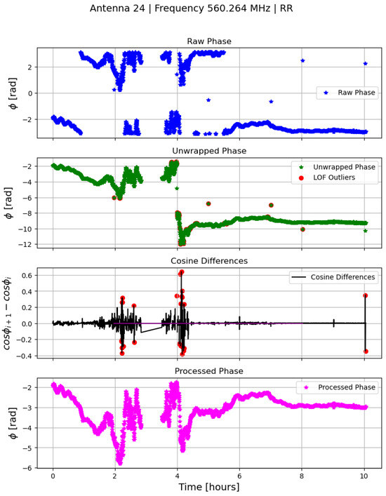
Figure 1.
(First row) The raw phase at 560.26 MHz for antenna 24, RR polarization, as a function of time. (Second row) The unwrapped phases with LOF outliers marked with red circles. (Third row) The difference between the cosine of the wrapped phase at a time step i and the next time step as a function of time, which is used to determine spikes in the phase data. Flagged spikes are highlighted with red circles. (Fourth row) The processed unwrapped phases where outliers are flagged at the level.
The LOF score for time step t is defined as follows:
where represents the set of k-nearest neighbors in time, and is the local reachability density provided by the following:
where is the Euclidean distance in the phase space. We choose . We use the function LocalOutlierFactor (n_neighbors=100, contamination=“auto”) from scikit-learn6. Time steps with anomalous LOF scores are flagged and removed, and the missing data points are linearly interpolated to ensure temporal continuity.
Following Helmboldt et al. [7] to remove short phase jumps from the unwrapped phases (Figure 1, second row), we design a cosine filter to remove spurious jumps in the wrapped phase before unwrapping it. The idea is to track how much , where is the wrapped phase, changes from one time step to the next. If the change at a particular time step is unusually large (specifically, exceeding five times the standard deviation across all time steps for a given antenna), we flag that point as unreliable. These flagged time steps are left out during phase unwrapping. Later, any gaps caused by the flagged points are filled in by interpolating the unwrapped phase values from the surrounding good data points. The final, cleaned phase solutions exhibit a substantial reduction in phase jumps and outliers. An example of this improvement for antenna 24 is shown in the bottom row of Figure 1.
The instrumental phase includes the error associated with the delays, the actual source position, and the offset of the antenna’s line of sight. These vary relatively slowly in time in comparison to ionospheric time fluctuations. We model instrumental effects using a continuum subtraction approach following Helmboldt et al. [7]. We treat ionospheric fluctuations as features superimposed on a smooth continuum consisting of the instrumental phases, which vary relatively slowly with time. We perform continuum subtraction for each antenna, band, and polarization by smoothing the unwrapped phases using a one-hour-wide boxcar window (Figure 2). This method effectively preserves apparent fluctuations while providing a reliable representation of the continuum. Unfortunately, we lack the capability to separate the slowly varying component of the ionospheric phase from instrumental effects. As a result, we can only measure fluctuations in TEC on relatively short timescales (≤1 h).
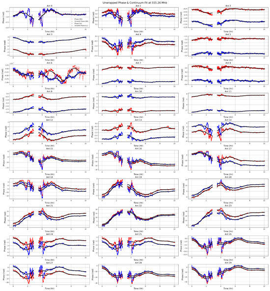
Figure 2.
This figure shows the unwrapped phases for polarization RR and LL, smoothed using a one-hour-wide boxcar window, which effectively preserves apparent fluctuations while providing a clear representation of the continuum. The red and blue points represent the unwrapped phases for correlation RR and LL, respectively, while the solid black lines show the smooth fits at 555.26 MHz. Note that the figure legend is included only in the first subplot to maintain overall clarity of the figure.
Furthermore, to estimate the smooth continuum component of the instrumental phase, we can utilize the two ends of the wide-band data–narrow frequency ranges (∼10 MHz each) separated by several MHz. The phase difference between the lower and upper sub-bands ( and ) is computed and scaled by , effectively suppressing ionospheric contributions that scale as . This procedure isolates the instrumental phase difference, as described in Mangla and Datta [15]. However, for our current wide-band dataset, we use the full frequency range and choose to fit a smooth model over time for each frequency channel. This method allows us to better account for how the instrument’s response changes with frequency and to capture a clean, smooth representation of the continuum signal over time [7]. We find the residual phases after continuum subtraction varies randomly around mean 0, with a scatter of radians for the central square GMRT antennas. In contrast, for the arm antennas, the maximum scatter in residual phases is around radians (Figure 3). We encounter a period of rapid phase and amplitude variation between approximately 19:30 and 21:45 IST. This significantly degrades the data quality, particularly during the interval from 20:15 to 20:55 IST (IST), which corresponds to the ∼45-m gap in our analysis. The possible causes are radio frequency interference (RFI) or some instrumental issues (drift due to the LO (local oscillator) unlock, bank-end issues, etc.), which can also cause rapid phase jumps. These fluctuations are significantly stronger than the neighboring time steps, so we consider the data to be unreliable and flag this time range. Residual RFIs may impact nearby time ranges, and to a large extent, the residual phases show an increase in scatter for all antennas within the 2 to 4 h range compared to the rest of the night’s data. It is also possible that the ionosphere is more active during this period, leading to the detection of large-scale traveling ionospheric disturbances (TIDs) or corruption of the visibility phases by ionospheric scintillations [3,24]. Further, around evening time in the Indian sector, both EIA crests intensify due to sunset conditions. This enhancement leads to the development of plasma bubbles, which can spread across the EIA trough and collapsing crests [14]. Strong scintillations during this time are also reported in the GMRT observation log file.
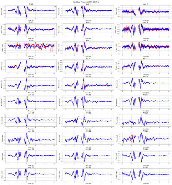
Figure 3.
The residual phases after the smooth continuum is removed at 555.26 MHz. Note that the figure legend is included only in the first subplot to maintain overall clarity of the figure.
3. Obtaining Ionospheric Information from Calibration Phases
After removing the instrumental component, we convert the residual phases for each antenna and polarization to differential TEC () using the scaling factor , where is in units of Hz. We calculate the median using all available values across frequency channels and both polarizations. To estimate the uncertainty, we use the median absolute deviation (MAD) computed at each time step for each antenna across all available frequency channels and polarization data (898 data points per time step). We report the median values to reduce the influence of any remaining outliers in the data.
The resulting values for each antenna as a function of time are shown in Figure 4 for the central square antennas, in Figure 5 for the eastern and southern antennas, and in Figure 6 for the northwestern arm. The uGMRT data typically achieve less than mTECU (≤mTECU) uncertainty for the central square antennas, whereas the variation, represented by the MAD values, is around a few mTECU ((1 mTECU = TECU)) for the arm antennas.
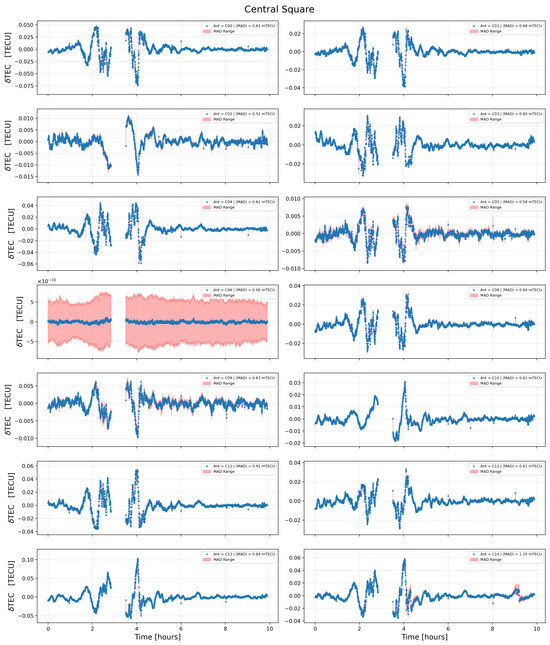
Figure 4.
For each antenna in the GMRT central square, this figure shows the along the antenna’s line of sight with respect to that of the reference antenna (‘C06’). The MAD values are also displayed in each panel to represent the estimated uncertainty.
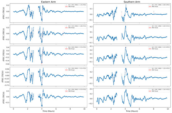
Figure 5.
Similar to Figure 4, but along the eastern and southern arm of GMRT.
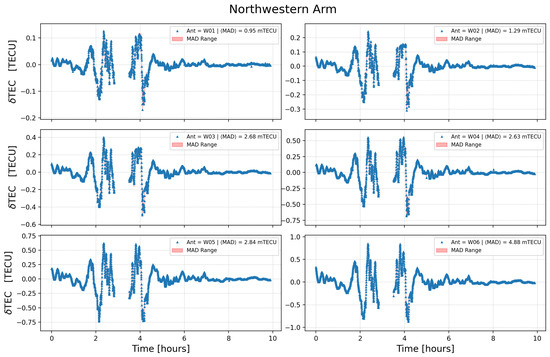
Figure 6.
Analogous to Figure 4, but along the northwestern arm of GMRT.
To independently verify whether our estimates are affected by residual RFI, we analyze a subset of data spanning the frequency range 590–615 MHz using AOFlagger [25] instead of the CASA flagging routine and applying a Lua strategy file7 for RFI detection and removal. We observe very similar variations over time for both the central square (Figure A1) and arm antennas of the GMRT. Based on this consistency, we proceed with the CASA-flagged data for the remainder of our analysis.
The differential TEC measured along the three arms of the GMRT exhibits slightly different patterns. In general, the arm antennas show stronger and slower fluctuations, which are characteristic features of traveling ionospheric disturbances (TIDs) [26]. This behavior could result from a large-scale wave moving through the ionosphere along with smaller waves or from multiple waves propagating in different directions. Later, when we compute the spatial gradient (Section 3.1), we aim to better decipher the dominant component, either east–west or north–south, of the TIDs. We plan to explore these patterns further using spectral analysis in a future study [27,28].
Unwrapped, continuum-subtracted phase differences between antennas can be used to track the temporal variation in across uGMRT baselines. We fit the phase difference using the model . Here, represents the ionospheric conversion factor, is the observing frequency in Hz, and denotes the difference in integrated ionospheric electron content (in TECU) along the lines of sight to antennas i and j [12]. For instruments with large bandwidths, this model allows us to exploit the wavelength dependence to better separate residual instrumental phases (which scale as ) from the ionospheric phase (which scales as ).
Two essential geometric corrections must be applied to the antenna positions and measurements to more accurately reflect actual ionospheric conditions. Since the observations of 3C48 include times when the source is relatively close to the horizon, a plane-parallel approximation is insufficient. Instead, a thin-shell approximation is used, in which the ionosphere is modeled as a thin layer at the height of maximum electron density, , as determined by the international reference ionosphere (IRI) model8 [29] for the corresponding dates and times of the observations (see Figure A2).
The first correction involves converting the ground-based antenna positions to their projected positions within the ionosphere. In a non-plane-parallel atmosphere, these positions vary with the elevation of the observed source. For a spherical ionospheric shell, a “pierce point” can be defined for each antenna, where the line of sight to the source intersects the ionosphere. The relative positions of these pierce points, referenced to the center of the array, serve as the projected positions within the ionosphere. We follow Appendix A of Helmboldt et al. [7] to estimate the projected GMRT antenna coordinates onto the ionospheric thin shell at each time step during the observation.
The second correction accounts for the increased path length through the ionosphere when the observed source is closer to the horizon. We convert the slant TEC (sTEC) values to vertical TEC (vTEC) values by applying a slant factor, , where is the angle between the line of sight from the GMRT to the source and the vertical line from the ionospheric pierce point to the point on the Earth’s surface directly beneath it [7].
Figure 7 shows a representative example of the fitted differential vTEC values for both the central square antennas (baselines ≤ 1.4 km) and the arm antennas, using antenna ‘C06’ as the reference. The color scale represents the baseline length. The fitting errors are displayed in the bottom panel of Figure 7. We observe temporally varying ionospheric effects that are spatially coherent across antennas, even on short baselines ( 1 km). A principal component analysis (PCA) of the time series of differential TEC () shows that just five principal components explain nearly of the total variance. Typically, for the core baselines, the values vary within ±0.1 TECU, whereas for the remote baselines (baselines ≥ 1.4 km), the variation is approximately ±1.0 TECU. The fitting errors in are approximately 100 times smaller (see Figure 7). For the central square baselines, the uncertainty (MAD) is around 0.0023 TECU, increasing to ∼0.0147 TECU for the arm antennas.
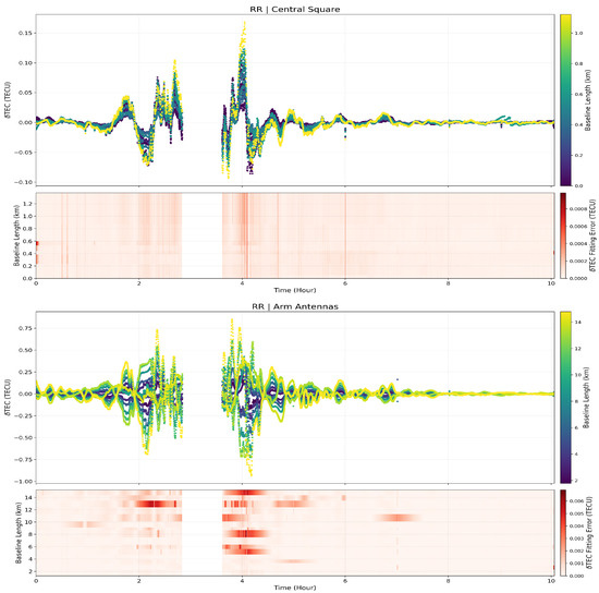
Figure 7.
Differential TEC () of uGMRT antennas relative to the refant antenna ‘C06’ over time. The color bar represents baseline length. (Top row) Central square baselines. (Bottom row) Longer arm baselines.
It is important to note that the accuracy of the TEC solutions derived using this method is limited by second-order phase effects [12], including the non-linear phase behavior with frequency, imperfections in the sky model, and cable reflections. Such higher-order effects tend to be more significant at frequencies below 100 MHz [24].
Results from the MWA interferometer have shown that accurately modeling small-scale ionospheric features requires a significantly denser network of global navigation satellite system (GNSS) stations. However, the region surrounding the GMRT site has very few of these stations; the closest known GNSS station with publicly available data is located in Hyderabad, approximately 500 km away. This sparse coverage makes it challenging to capture fine-scale ionospheric variability in the area.
Although total electron content (TEC) maps provided by the international GNSS service [30,31] can be used to infer absolute TEC values (Figure A4), their effectiveness is limited. This limitation arises due to uncertainties in the projected magnetic field parameters and the relatively low temporal resolution of these models, which range from tens of minutes to hours. As a result, they are not ideal for assessing real-time ionospheric conditions during low-frequency interferometric radio observations.
Moreover, at Band-4 frequencies, our datasets lack the sensitivity required to estimate second-order ionospheric effects, such as those caused by Faraday rotation. This further complicates efforts to derive absolute vTEC values from differential TEC () measurements [24].
3.1. TEC Gradients
The GMRT measures differential the TEC between pairs of antennas. As a result, it is only inherently sensitive to variations in the TEC gradient. However, the geometry of the array makes it difficult to determine the absolute TEC gradient at individual antenna locations.
To overcome this, reconstructing the full TEC gradient requires a somewhat heuristic approach [7,15]. This reconstruction step is essential for accurately characterizing TEC fluctuations. Without it, the raw time series can only be interpreted meaningfully in the spectral domain. Even then, strong assumptions, such as the presence of a single plane wave, must be made [8].
Unlike standard interferometric imaging, which involves transforming and deconvolving visibility data to reconstruct sky images, studying ionospheric gradients demands accounting for how each antenna’s line of sight intersects the ionospheric shell. This introduces an additional layer of geometric complexity. Nonetheless, by leveraging the rotation of the Earth and the drift of ionospheric irregularities, we can map temporal fluctuations into spatial structures. However, in contrast to predictable Earth rotation synthesis, irregular drift speeds and directions of ionospheric features introduce significant mapping uncertainties. A widely adopted strategy involves decomposing the time series into spectral components and analyzing how these spectral modes manifest spatially across the array. This method facilitates the estimation of key parameters of ionospheric features, such as their scale, drift velocity, and propagation angle [27,28].
As outlined in Section 3, two geometric transformations are employed to bring the observed gradients in line with their vertical equivalents. First, antenna coordinates are projected onto their corresponding ionospheric pierce points. Second, a slant-to-vertical correction is applied to compensate for the varying elevation angle of the source 3C48 during the observation period.
After applying geometric corrections to both the antenna positions and the values, we aim to reconstruct the full two-dimensional TEC gradient at each antenna and time step. We do not assume a specific structure, such as a plane wave. Instead, we take advantage of the fact that the GMRT array is small compared to the typical scale of ionospheric disturbances. This allows us to approximate the TEC surface using a low-order Taylor expansion. We examine the data over several time steps. The results show that the TEC structure is well represented by a second-order, two-dimensional Taylor series. The corresponding polynomial form is as follows:
Here, x and y represent the antenna positions in the north–south and east–west directions, respectively. These positions are projected onto the ionospheric surface. The projection is carried out at the estimated peak height of the ionosphere, as determined by the IRI model.
For robust parameter estimation, we use the differences from all 406 unique antenna pairs at each time step. This allows us to fully utilize the available data.
We model the differential TEC between antenna pairs using a second-order polynomial expansion in the projected antenna coordinates:
This can be written in matrix form as follows:
where is the polynomial coefficient vector, is the vector of observed differential TEC values, and is the mapping matrix, with rows based on the antenna coordinates, as presented in Equation (5).
We also account for the uncertainties in the derived values. To optimize the polynomial coefficients over time, we apply a weighted least squares method. The weight matrix is a diagonal matrix. Each diagonal element corresponds to the inverse of the variance of the differential TEC measurements:
Here, denotes the standard deviation of the i-th differential TEC measurement. It is worth noting that additional residual systematics may contribute to the overall uncertainty; however, we neglect these effects in our analysis, as they are difficult to quantify a priori.
We solve the following regularized least squares problem using a small regularization parameter for numerical stability:
which yields the following solution:
We apply standard sigma-clipping during the fitting process. Antenna pairs with absolute residuals greater than are rejected at each time step. The rms of the fit residuals is calculated. This procedure is repeated up to 10 times. Between 0 and a maximum of 63 baselines are rejected per time step. To preserve small temporal and spatial changes, each time step is fitted independently.
Figure 8 displays the evolution of the fitted coefficients over time. Notably, and , representing the linear TEC gradients in the north–south and east–west directions, exhibit large amplitude oscillations, especially at the beginning of the observation. These variations are consistent with the fluctuations seen in Figure 4, Figure 5 and Figure 6. The coefficient, related to the north–south gradient, shows fluctuations up to TECU, particularly during sunset. This behavior aligns with the known properties of medium-scale traveling ionospheric disturbances (MSTIDs) [26]. Observation logs also suggest increased scintillation during this interval. Higher-order polynomial terms capture localized, finer-scale features that are more prominent at later times.
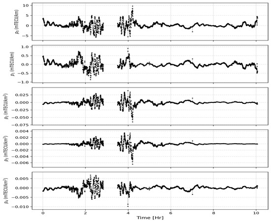
Figure 8.
The fitted polynomial coefficients (Equation (5)) as a function of time.
Smaller and more transient TEC gradient structures are observed in the middle portion of the observation (Figure A3). The north–south gradient shows more variability than the east–west component. For antennas on the GMRT’s southern arm, the peak gradient amplitude reaches approximately TECU/km. This behavior is indicative of medium-scale traveling ionospheric disturbances (MSTIDs), which typically arise during the evening and night-time [7,15]. These small-scale features may reflect rippling in MSTID wavefronts, turbulent mixing from ion-neutral interactions, or localized enhancements, such as sporadic-E layers [32]. Due to the irregular layout of central square antennas, resolving the directionality of TEC gradients is difficult in this region. Therefore, here, these antennas are excluded (Figure A3).
3.2. Structure Function
In this subsection, we characterize the spatial structure of the ionosphere using the phase structure function, defined as follows:
where is the separation distance, and denotes the statistical expectation value.
The phase structure function is often modeled as a power law based on Kolmogorov’s theory of turbulence:
where is the diffractive scale of the ionosphere. According to Kolmogorov’s theory for inertial-range turbulence, the power-law index is expected to be . A smaller diffractive scale corresponds to stronger phase fluctuations across the field of view, resulting in reduced temporal coherence of the signal [33].
Deviations from the Kolmogorov scaling can occur due to non-turbulent ionospheric structures such as traveling ionospheric disturbances (TIDs) [34] or field-aligned density ducts [35]. For example, wave-like TIDs typically yield slopes of .
Figure 9 presents the measured phase structure function along with the best-fit model. We obtain a power-law index of , which is slightly steeper than the Kolmogorov value, suggesting the presence of additional ionospheric structures. The fitted diffractive scale is km, which corresponds to the spatial scale over which the phase variance reaches .
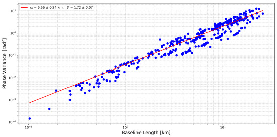
Figure 9.
Phase structure function of the ionosphere derived from differential TEC values converted to phases at 600 MHz, the blue points are the measured phase variance shown as a function of baseline length. The red solid line is the fitted power law model as in Equation (11).
Consistent with the LOFAR observations of Mevius et al. [12], we observe a band-like pattern in the structure function, indicative of anisotropic ionospheric irregularities. A full two-dimensional structure function analysis using uGMRT data would help determine whether these structures align with Earth’s magnetic field [12]. We leave this investigation to future studies, where we plan to conduct a detailed 2D structure–function analysis across multiple uGMRT bands.
4. Summary and Conclusions
In this study, we observed the bright flux calibrator 3C48 using uGMRT Band-4 data centered at 600 MHz, demonstrating the telescope’s unique ability to probe ionospheric activity at low latitudes. Our analysis shows that GMRT can measure differential TEC with sub-mTECU precision on 10-second timescales, offering significantly greater sensitivity to TEC fluctuations than GPS-based relative TEC measurements [26]. The accuracy of these estimates could be further enhanced with improved sky and instrument modeling. Similar levels of precision have been achieved in mid-latitude studies with the VLA [7] and LOFAR [12].
We found that for central square baselines with spatial scales ≤ 1.4 km, TEC fluctuations can be measured with a median absolute deviation (MAD) of 2.3 mTECU. In contrast, precision drops by over an order of magnitude on longer baselines (≥1.4 km). This decrease is likely due to small-scale ionospheric structures decorrelating over larger distances, which reduces signal coherence and limits sensitivity to differential TEC () variations. Factors such as system temperature, pointing accuracy, and variations in antenna beam shapes between central and remote antennas may also impact phase stability, further influencing the accuracy of estimates.
During our observations, we recorded significant fluctuations in the differential total electron content (), with amplitudes increasing rapidly after the local sunset at approximately 17:56 Indian standard time (IST). This timing aligns with the ionospheric transition from a photoionization-driven regime to one dominated by recombination, a period known to foster enhanced plasma instabilities [36]. Moreover, pre-reversal enhancement increases the upward movement of charged particles (plasma) in the ionosphere after sunset. This strengthens the equatorial ionization anomaly (EIA), causing more electrons to accumulate in the two crest regions on either side of the magnetic equator. As radio signals pass through the resulting plasma bubbles, they become scattered, leading to amplitude and phase scintillations [14].
We quantified the spatial variability of the ionosphere using the phase structure function and found that it follows power-law behavior with a slope of , which is slightly steeper than the Kolmogorov prediction of . This suggests the presence of additional, possibly non-turbulent structures such as traveling ionospheric disturbances (TIDs) or field-aligned density ducts [35]. The derived diffractive scale of km indicates significant phase fluctuations across the field of view, with implications for signal coherence in low-frequency interferometric observations. The observed anisotropic features in the structure–function further motivate a two-dimensional analysis to investigate the potential alignment of ionospheric irregularities with Earth’s magnetic field, which we defer to future studies.
To evaluate the spatial coherence of ionospheric fluctuations across the GMRT array, we applied principal component analysis to the time series of differential TEC () measured along each baseline. Interestingly, just five principal components explained nearly of the total variance. This indicates that the ionospheric perturbations are highly structured and primarily governed by a small number of dominant temporal modes. Such a low-rank representation is consistent with a spatially coherent ionospheric screen, where fluctuations are strongly correlated across the array, even over relatively short baselines. This structure supports the application of reduced-order ionospheric models in calibration and points toward the presence of large-scale physical phenomena, such as traveling ionospheric disturbances or global TEC gradients. However, to robustly identify the nature of these fluctuations, such as their size, speed, and direction, and to distinguish them from other ionospheric processes, a more detailed spectral analysis of the time series is essential [27].
The polynomial-based method described in Section 3.1 successfully captures the large-scale structure of the two-dimensional TEC gradients across the array. Although this technique lacks sensitivity to small-scale or rapidly varying features, it effectively models the broader, more dominant fluctuations, i.e., those with larger amplitudes and longer temporal or spatial scales, which are present in the TEC gradient field. Given that measurements are accurate to approximately TECU and the average distance between antennas is around 3 km, this translates to a typical uncertainty in the estimated TEC gradient of roughly ∼ TECU per kilometer.
Finally, we conclude that the GMRT’s geographic location makes it particularly advantageous for probing ionospheric behavior, a key factor in enhancing the performance of low-frequency radio astronomy [6,24]. If ionospheric systematics can be effectively captured using a small set of parameters, the number of free parameters in calibration can be significantly reduced, especially for observations with low signal-to-noise ratios. This approach paves the way for improved sensitivity and resolution in radio imaging [37]. Similar ionospheric studies will soon become feasible, with upcoming next-generation instruments, such as the SKA, expected to be operational in the coming years.
Author Contributions
D.B. and A.G. coordinated the observational campaign, performed the radio data analyses and interpretations, and led the writing of the paper. D.B., A.G., S.K.M. and P.G. reviewed the draft and contributed to the writing of the manuscript. All authors have read and agreed to the published version of the manuscript.
Funding
All the authors wish to acknowledge funding provided under the SERB-SURE grant SUR/2022/000595 of the Science and Engineering Research Board, a statutory body of the Department of Science and Technology (DST), Government of India.
Data Availability Statement
The observed data are publicly available after a proprietary period of 18 months through the GMRT data archive9 under the proposal code 47_003.
Acknowledgments
We thank the staff of GMRT for making this observation possible. GMRT is run by the National Centre for Radio Astrophysics (NCRA) of the Tata Institute of Fundamental Research (TIFR). We thank all the reviewers whose comments helped us improve the overall quality of the paper. The authors utilized ChatGPT for AI-assisted copy editing and improving the manuscript’s language. AG would like to thank IUCAA, Pune, for providing support through the associateship programme, including access to the computational facility at IUCAA.
Conflicts of Interest
The authors declare no competing financial interests.
Appendix A
Appendix A.1. δ TEC vs. Time for Central Square Antennas (CASA Flagging vs. AOFlagger)
In this section, we compare the temporal variation of the differential total electron content (TEC), as obtained using two different radio frequency interference (RFI) mitigation strategies: CASA’s internal flagging algorithm and the AOFlagger tool. The focus is restricted to the GMRT’s central square antennas, and the arm antennas also show a similar behavior. The figure displays the TEC values obtained from each flagging method, allowing an assessment of how RFI mitigation influences ionospheric phase extraction. The red vertical dashed line marks the period during which scintillation was reported in the observation log.
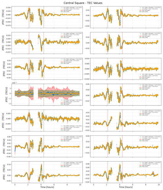
Figure A1.
The blue triangles and orange circles illustrate the temporal variation in for central square antennas. CASA flagging was applied for the blue data points, while AOFlagger was used for the orange ones. The red vertical dashed line indicates the time slots during which scintillation was reported in the GMRT observation log file.
Appendix A.2. IRI-Predicted Peak Height and Slant TEC Scaling Factor
This section presents model-based predictions of the ionospheric peak electron density height using the international reference ionosphere (IRI) model. The top panel of the figure shows how the peak height evolves over the course of the observation. This information is critical for determining the ionospheric pierce point geometry. In the bottom panel, we plot the corresponding slant-to-vertical TEC conversion factor, computed assuming a thin-shell ionospheric model at the predicted heights.
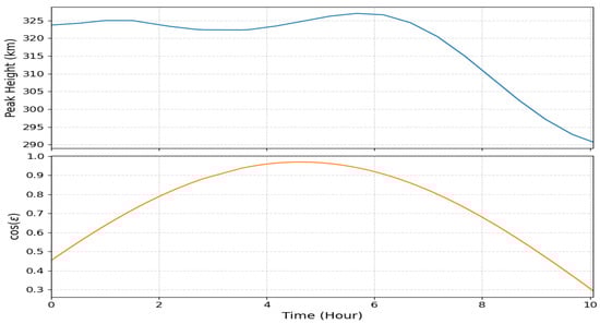
Figure A2.
(Top) Temporal variation in the peak height of the maximum electron density at the ionospheric pierce points, as predicted by the IRI model on 23 November 2024 (https://www.ionolab.org/iriplasonline/). (Bottom) Associated scaling factor used to convert slant TEC measurements to their vertical equivalents, assuming a thin-shell ionosphere positioned at the heights shown above.
Appendix A.3. Projected TEC Gradient
This section shows the TEC gradient projected along the GMRT arms, estimated from polynomial fits to TEC time series data between antenna pairs. Gradients are plotted for the north–south (blue) and east–west (orange) directions, revealing the anisotropic structure of ionospheric variations.
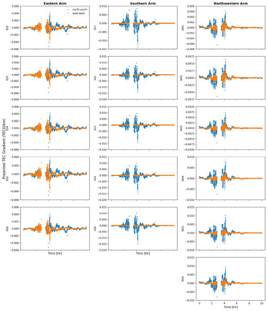
Figure A3.
This figure shows the projected TEC gradients estimated from the polynomial coefficients for the GMRT arm antennas along the north–south (blue circles) and east–west (orange triangles) directions. Note that the figure legend is included only in the first subplot to maintain overall clarity of the figure.
Appendix A.4. Absolute Vertical TEC from IGS Models
The ionospheric total electron content (TEC) estimates on an hourly basis from different IONEX data centers. We used the Spinifex library (https://git.astron.nl/RD/spinifex, accessed on 23 November 2024) to extract vertical TEC (vTEC) values along the line of sight to the radio source 3C48, as seen from the GMRT site. For this estimate, we adopted a single-layer ionospheric model at a height of 300 km.
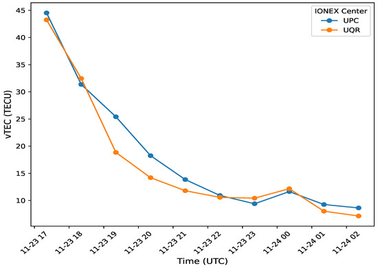
Figure A4.
This figure presents hourly estimates of the ionospheric total electron content (TEC) from various IGS models during our observation period. The overall trend aligns with our differential TEC measurements, showing greater ionospheric variability at the beginning of the observation, which gradually decreases toward the end.
Notes
| 1 | |
| 2 | |
| 3 | |
| 4 | |
| 5 | |
| 6 | |
| 7 | |
| 8 | |
| 9 |
References
- Thompson, A.R.; Moran, J.M.; Swenson, G.W., Jr. Interferometry and Synthesis in Radio Astronomy, 2nd ed.; Wiley-Interscience: Hoboken, NJ, USA, 2001. [Google Scholar]
- Mangum, J.G.; Wallace, P. Atmospheric Refractive Electromagnetic Wave Bending and Propagation Delay. Publ. Astron. Soc. Pac. 2015, 127, 74. [Google Scholar] [CrossRef]
- Fallows, R.A.; Forte, B.; Astin, I.; Allbrook, T.; Arnold, A.; Wood, A.; Dorrian, G.; Mevius, M.; Rothkaehl, H.; Matyjasiak, B.; et al. A LOFAR observation of ionospheric scintillation from two simultaneous travelling ionospheric disturbances. J. Space Weather Space Clim. 2020, 10, 10. [Google Scholar] [CrossRef]
- Opio, P.; D’ujanga, F.; Ssenyonga, T. Latitudinal variation of the ionosphere in the African sector using GPS TEC data. Adv. Space Res. 2015, 55, 1640–1650. [Google Scholar] [CrossRef]
- Lonsdale, C.J. Configuration Considerations for Low Frequency Arrays. In From Clark Lake to the Long Wavelength Array: Bill Erickson’s Radio Science; Astronomical Society of the Pacific Conference Series; Kassim, N., Perez, M., Junor, W., Henning, P., Eds.; Astronomical Society of the Pacific: Cambridge, MA, USA, 2005; Volume 345, p. 399.
- Intema, H.T.; van der Tol, S.; Cotton, W.D.; Cohen, A.S.; van Bemmel, I.M.; Röttgering, H.J.A. Ionospheric calibration of low frequency radio interferometric observations using the peeling scheme—I. Method description and first results. Astron. Astrophys. 2009, 501, 1185–1205. [Google Scholar] [CrossRef]
- Helmboldt, J.F.; Lazio, T.J.W.; Intema, H.T.; Dymond, K.F. High-precision measurements of ionospheric TEC gradients with the Very Large Array VHF system. Radio Sci. 2012, 47, RS0K02. [Google Scholar] [CrossRef]
- Jacobson, A.R.; Erickson, W.C. A method for characterizing transient ionospheric disturbances using a large radiotelescope array. A&A 1992, 257, 401–409. [Google Scholar]
- Cohen, A.S.; Röttgering, H.J.A. Probing fine-scale ionospheric structure with the Very Large Array radio telescope. Astron. J. 2009, 138, 439. [Google Scholar] [CrossRef]
- Jordan, C.H.; Murray, S.; Trott, C.M.; Wayth, R.B.; Mitchell, D.A.; Rahimi, M.; Pindor, B.; Procopio, P.; Morgan, J. Characterization of the ionosphere above the Murchison Radio Observatory using the Murchison Widefield Array. Mon. Not. R. Astron. Soc. 2017, 471, 3974–3987. [Google Scholar] [CrossRef]
- Helmboldt, J.F.; Lane, W.M.; Cotton, W.D. Climatology of midlatitude ionospheric disturbances from the Very Large Array Low-frequency Sky Survey. Radio Sci. 2012, 47, S5008. [Google Scholar] [CrossRef]
- Mevius, M.; van der Tol, S.; Pandey, V.N.; Vedantham, H.K.; Brentjens, M.A.; de Bruyn, A.G.; Abdalla, F.B.; Asad, K.M.B.; Bregman, J.D.; Brouw, W.N.; et al. Probing ionospheric structures using the LOFAR radio telescope. Radio Sci. 2016, 51, 927–941. [Google Scholar] [CrossRef]
- Appleton, E.V. Two Anomalies in the Ionosphere. Nature 1946, 157, 691. [Google Scholar] [CrossRef]
- Balan, N.; Institute of Geology and Geophysics, Chinese Academy of Sciences; Liu, L.; Le, H. A brief review of equatorial ionization anomaly and ionospheric irregularities. Earth Planet. Phys. 2018, 2, 257–275. [Google Scholar] [CrossRef]
- Mangla, S.; Datta, A. Study of the equatorial ionosphere using the Giant Metrewave Radio Telescope (GMRT) at sub-GHz frequencies. Mon. Not. R. Astron. Soc. 2022, 513, 964–975. [Google Scholar] [CrossRef]
- Gupta, Y.; Ajithkumar, B.; Kale, H.S.; Nayak, S.; Sabhapathy, S.; Sureshkumar, S.; Swami, R.V.; Chengalur, J.N.; Ghosh, S.K.; Ishwara-Chandra, C.H.; et al. The upgraded GMRT: Opening new windows on the radio Universe. Curr. Sci. 2017, 113, 707–714. [Google Scholar] [CrossRef]
- Perley, R.A.; Butler, B.J. An Accurate Flux Density Scale from 1 to 50 GHz. Astrophys. J. Suppl. Ser. 2013, 204, 19. [Google Scholar] [CrossRef]
- CASA Team; Bean, B.; Bhatnagar, S.; Castro, S.; Donovan Meyer, J.; Emonts, B.; Garcia, E.; Garwood, R.; Golap, K.; Gonzalez Villalba, J.; et al. CASA, the Common Astronomy Software Applications for Radio Astronomy. Publ. Astron. Soc. Pac. 2022, 134, 114501. [Google Scholar] [CrossRef]
- Smirnov, O.M. Revisiting the radio interferometer measurement equation. I. A full-sky Jones formalism. A&A 2011, 527, A106. [Google Scholar] [CrossRef]
- Arora, B.S.; Morgan, J.; Ord, S.M.; Tingay, S.J.; Bell, M.; Callingham, J.R.; Dwarakanath, K.S.; For, B.Q.; Hancock, P.; Hindson, L.; et al. Ionospheric Modelling using GPS to Calibrate the MWA. II: Regional Ionospheric Modelling using GPS and GLONASS to Estimate Ionospheric Gradients. Publ. Astron. Soc. Aust. 2016, 33, e031. [Google Scholar] [CrossRef]
- Swarup, G.; Ananthakrishnan, S.; Kapahi, V.K.; Rao, A.P.; Subrahmanya, C.R.; Kulkarni, V.K. The Giant Metre-Wave Radio Telescope. Curr. Sci. 1991, 60, 95. [Google Scholar]
- Pearson, T.J.; Perley, R.A.; Readhead, A.C.S. Compact radio sources in the 3C catalog. Astron. J. 1985, 90, 738–755. [Google Scholar] [CrossRef]
- Scaife, A.M.M.; Heald, G.H. A broad-band flux scale for low-frequency radio telescopes. Mon. Not. R. Astron. Soc. 2012, 423, L30–L34. [Google Scholar] [CrossRef]
- de Gasperin, F.; Mevius, M.; Rafferty, D.A.; Intema, H.T.; Fallows, R.A. The effect of the ionosphere on ultra-low-frequency radio-interferometric observations. Astron. Astrophys. 2018, 615, A179. [Google Scholar] [CrossRef]
- Offringa, A.R.; van de Gronde, J.J.; Roerdink, J.B.T.M. A morphological algorithm for improving radio-frequency interference detection. Astron. Astrophys. 2012, 539, A95. [Google Scholar] [CrossRef]
- Hernández-Pajares, M.; Juan, J.M.; Sanz, J. Medium-scale traveling ionospheric disturbances affecting GPS measurements: Spatial and temporal analysis. J. Geophys. Res. Space Phys. 2006, 111. [Google Scholar] [CrossRef]
- Helmboldt, J.F.; Lazio, T.J.W.; Intema, H.T.; Dymond, K.F. A new technique for spectral analysis of ionospheric TEC fluctuations observed with the Very Large Array VHF system: From QP echoes to MSTIDs. Radio Sci. 2012, 47, RS0L02. [Google Scholar] [CrossRef]
- Mangla, S.; Datta, A. Spectral Analysis of Ionospheric Density Variations Measured With the Large Radio Telescope in the Low-Latitude Region. Geophys. Res. Lett. 2023, 50, e2023GL103305. [Google Scholar] [CrossRef]
- Bilitza, D.; Pezzopane, M.; Truhlik, V.; Altadill, D.; Reinisch, B.W.; Pignalberi, A. The International Reference Ionosphere Model: A Review and Description of an Ionospheric Benchmark. Rev. Geophys. 2022, 60, e2022RG000792. [Google Scholar] [CrossRef]
- Orús, R.; Hernández-Pajares, M.; Juan, J.M.; Sanz, J. Improvement of global ionospheric VTEC maps by using kriging interpolation technique. J. Atmos. Sol. Terr. Phys. 2005, 67, 1598–1609. [Google Scholar] [CrossRef]
- Hernández-Pajares, M.; Juan, J.M.; Sanz, J.; Orus, R.; Garcia-Rigo, A.; Feltens, J.; Komjathy, A.; Schaer, S.C.; Krankowski, A. The IGS VTEC maps: A reliable source of ionospheric information since 1998. J. Geod. 2009, 83, 263–275. [Google Scholar] [CrossRef]
- Coker, C.; Thonnard, S.E.; Dymond, K.F.; Lazio, T.J.W.; Makela, J.J.; Loughmiller, P.J. Simultaneous radio interferometer and optical observations of ionospheric structure at the Very Large Array. Radio Sci. 2009, 44. [Google Scholar] [CrossRef]
- Vedantham, H.K.; Koopmans, L.V.E. Scintillation noise in widefield radio interferometry. Mon. Not. R. Astron. Soc. 2015, 453, 925–938. [Google Scholar] [CrossRef]
- Vanvelthoven, P.F.J. Medium Scale Irregularities in the Ionospheric Electron Content. Ph.D. Thesis, Technical University of Eindhoven, Eindhoven, The Netherlands, 1990. [Google Scholar]
- Loi, S.T.; Murphy, T.; Cairns, I.H.; Menk, F.W.; Waters, C.L.; Erickson, P.J.; Trott, C.M.; Hurley-Walker, N.; Morgan, J.; Lenc, E.; et al. Real-time imaging of density ducts between the plasmasphere and ionosphere. Geophys. Res. Lett. 2015, 42, 3707–3714. [Google Scholar] [CrossRef]
- DasGupta, A.; Paul, A.; Ray, S.; Das, A.; Ananthakrishnan, S. A study of precursors to equatorial spread F using the Giant Meterwave Radio Telescope. Radio Sci. 2008, 43, RS5002. [Google Scholar] [CrossRef]
- de Gasperin, F.; Dijkema, T.J.; Drabent, A.; Mevius, M.; Rafferty, D.; van Weeren, R.; Brüggen, M.; Callingham, J.R.; Emig, K.L.; Heald, G.; et al. Systematic effects in LOFAR data: A unified calibration strategy. Astron. Astrophys. 2019, 622, A5. [Google Scholar] [CrossRef]
Disclaimer/Publisher’s Note: The statements, opinions and data contained in all publications are solely those of the individual author(s) and contributor(s) and not of MDPI and/or the editor(s). MDPI and/or the editor(s) disclaim responsibility for any injury to people or property resulting from any ideas, methods, instructions or products referred to in the content. |
© 2025 by the authors. Licensee MDPI, Basel, Switzerland. This article is an open access article distributed under the terms and conditions of the Creative Commons Attribution (CC BY) license (https://creativecommons.org/licenses/by/4.0/).