On Optimally Selecting Candidate Detectors with High Predicted Radio Signals from Energetic Cosmic Ray-Induced Extensive Air Showers

Abstract

Monte Carlo simulations of induced extensive air showers (EASs) by ultra-high-energy cosmic rays are widely used in comparison with measured events at experiments to estimate the main cosmic ray characteristics, such as mass, energy, and arrival direction. However, these simulations are computationally expensive, with running time scaling proportionally with the number of radio antennas included. The AugerPrime upgrade of the Pierre Auger Observatory will feature an array of 1660 radio antennas. As a result, simulating a single EAS using the full detector array will take weeks on a single CPU thread. To reduce the simulation time, detectors are commonly pre-selected based on their proximity to the shower core, using a selection ellipse based on the Cherenkov radiation footprint scaled by a fixed constant factor. While effective, this approach often includes many noisy antennas at high zenith angles, reducing computational efficiency. In this paper, we introduce an optimal method for selecting candidate detectors with high predicted signal-to-noise ratio for proton and iron primary cosmic rays, replacing the constant scaling factor with a function of the zenith angle. This approach significantly reduces simulation time—by more than 50% per CPU thread for the heaviest, most inclined showers—without compromising signal quality.

1. Introduction

Measurements of radio signals from cosmic ray-induced air showers were pioneered by the LOPES (LOFAR Prototype Station) experiment with its first results in 2005 [1], followed by the CODALEMA experiment [2,3]. It employed 10 dipole radio antennas (LOPES-10) co-located at the KASCADE experiment in Karlsruhe, Germany, which provided the trigger and well-calibrated information about properties of air shower characteristics. Compared to historical experiments, which were limited in terms of electronics in the late 1960s, LOPES has demonstrated the usability of the radio technique in modern cosmic ray experiments [4]. It provided an order of magnitude increase in bandwidth and time resolution, including digital filtering, and showed for the first time the interferometric imaging capabilities of the radio technique.

The LOPES experiment had developed further, growing to 30 antennas (LOPES-30), paving the way for a new and larger radio experiment, the Auger Engineering Radio Array (AERA), at the Pierre Auger Observatory [5] in Malargüe, Argentina. Similarly, AERA had started its measurements with 24 antennas covering an area of 0.5 ${\mathrm{km}}^2$, and it developed further to an increased area of 153 antennas, demonstrating that the radio detection technique works successfully in complement to the traditional methods used at the Pierre Auger Observatory, i.e., the water-Cherenkov detectors (WCDs) and the fluorescence telescopes [6]. Furthermore, the radio detection method has been proved to be suitable for measuring highly inclined air showers [7].

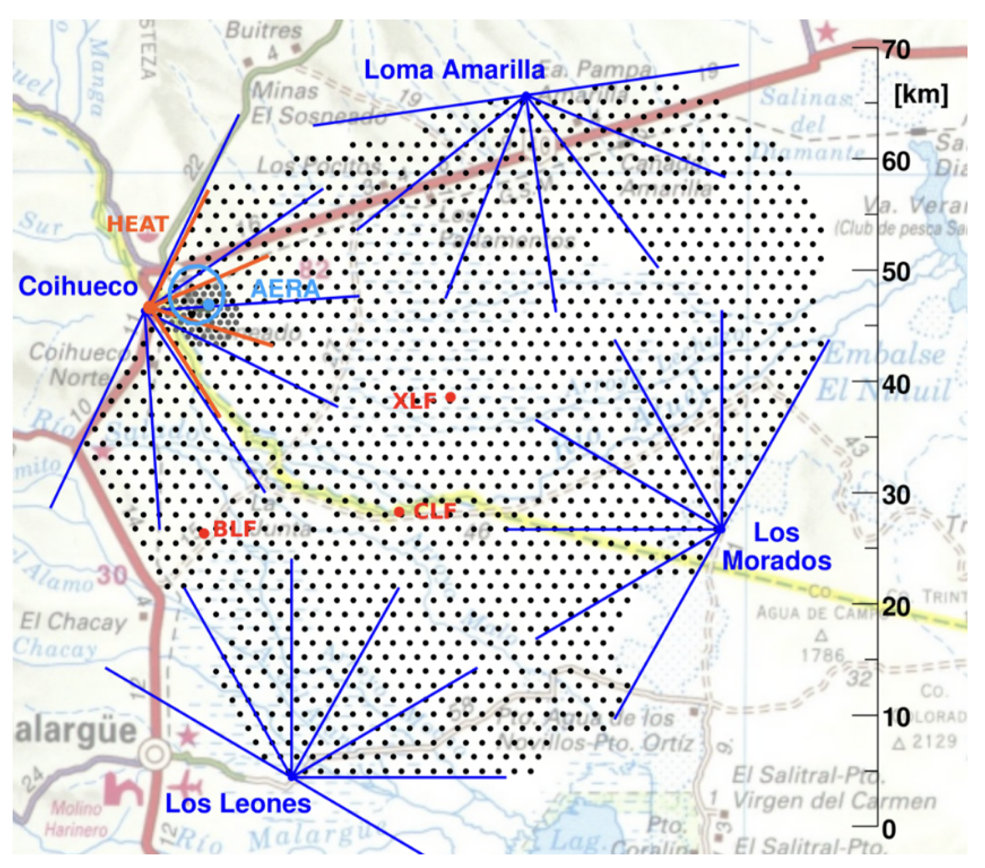
Since 2004, the Pierre Auger Observatory (Figure 1) has been observing ultra-high-energy cosmic rays (UHECRs) [8,9] in the southern sky with 1660 WCDs, covering an area of about 3000 ${\mathrm{km}}^2$, overlooked by 27 fluorescence telescopes arranged in four different locations. Currently, Auger is running in Phase II of data taking, also called AugerPrime [10], which, among other upgrades of the Observatory at the surface detector level, a radio antenna is placed on top of each WCD on the entire array, significantly increasing the total exposure of the experiment and complementarily facilitating mass-sensitive measurements.

The radio emission from cosmic ray-induced air showers is well understood nowadays, allowing one to disentangle between the two main radio emission mechanisms, the geomagnetic and the Askaryan effects [12]. Secondary electrons and positrons produced in the air shower particle cascade are, on the one hand, deflected by the Earth’s magnetic field, resulting in relativistically dipole radiation beamed into the forward direction, such as geosynchrotron radiation. On the other hand, there is a time variation in the negative charge excess in the shower front, which denotes Askaryan radiation.

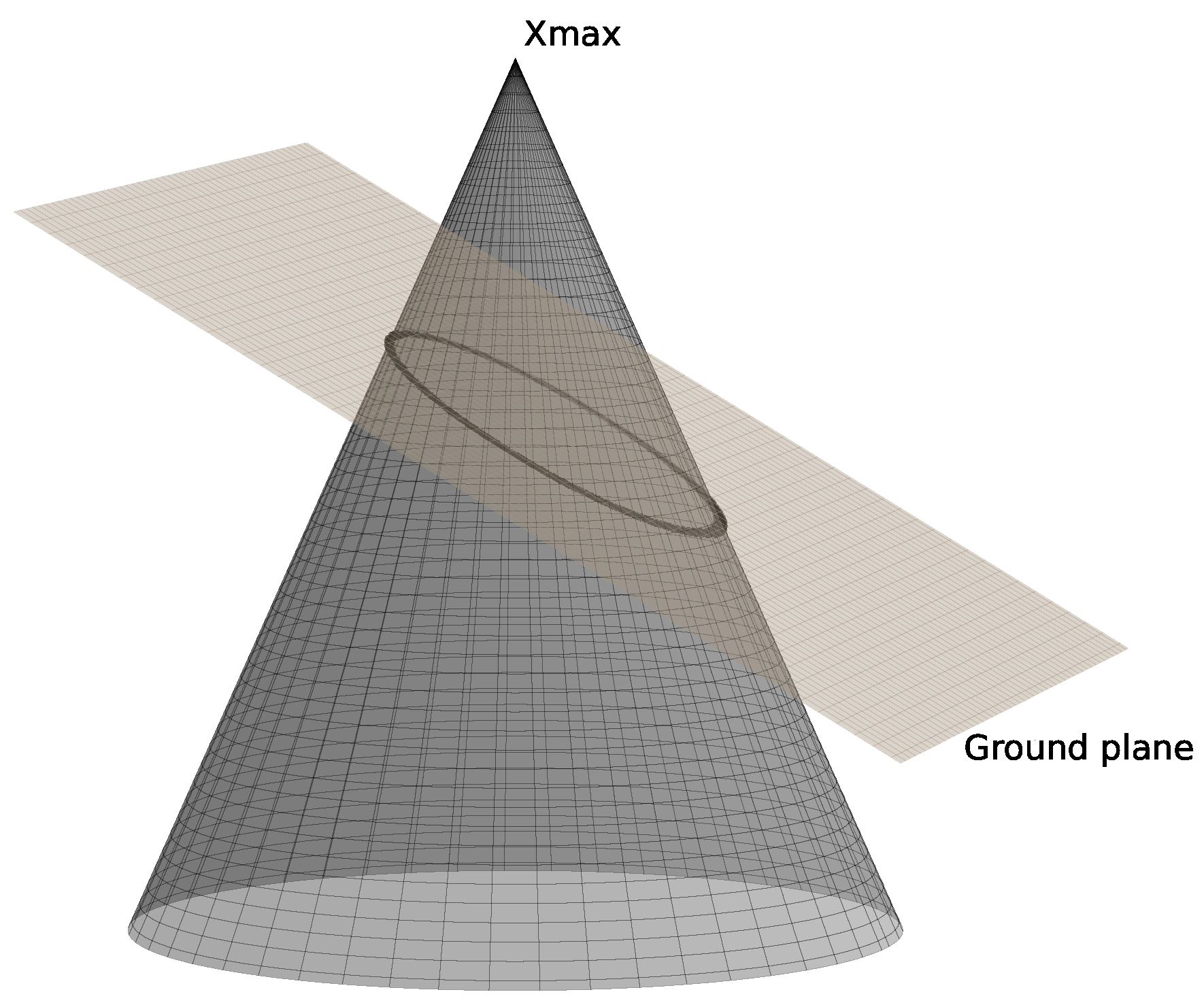
The strong radio signals emitted from air showers are projected onto the ground and arrive simultaneously in the order of nanoseconds [13]. The electromagnetic radiation produced when a charged particle travels through a dielectric medium at a velocity greater than the phase velocity of light in that medium—propagates in the direction of the shower axis as a conical wavefront, forming a Cherenkov-like effect of the radio emission with a ring (i.e., vertical air showers, see Equation (2)) or ellipse (i.e., inclined air showers, see Equation (3)) as a footprint on the ground [14] (Figure 2), starting—in a first approximation—from the maximum development of the air shower, i.e., ${\mathrm{X}}_{\max }$ [15], at an angle described by Equation (1), where c is the speed of light, v_p is the velocity of particle, and n is the medium refractive index, at the height of X_max. At ultra-relativistic speeds, the two velocities become approximately equal, and their ratio can be considered close to 1.

$${\varphi }_{\mathrm{Ch}}=arccos\left({\displaystyle \frac{1\times c}{n\times v_p}}\right)\approx arccos\left({\displaystyle \frac{1}{n}}\right)$$

(1)

If the zenith angle of the UHECR is approximately 0°, which means that the shower axis is perpendicular to the ground, its projection is a circle on the ground with the shower core at the center and a radius that can be easily calculated (Equation (2)), where ${\mathrm{D}}_{{\mathrm{X}}_{\max }}$ is the distance from the shower core to ${\mathrm{X}}_{\max }$.

$$r_{\mathrm{Cherenkov}}={\mathrm{D}}_{{\mathrm{X}}_{\max }}\times tan\left({\varphi }_{Ch}\right)$$

(2)

However, for zenith angles greater than 0°, the circular projection becomes elongated, producing an elliptical footprint on the ground. While the semi-minor axis ($r_{\mathrm{b}}$) remains the same, the semi-major axis ($r_{\mathrm{a}}$) is proportionally elongated with a factor depending on the zenith angle $\theta$ (Equation (3)) [17].

$$r_{\mathrm{a}}={\displaystyle \frac{r_{\mathrm{Cherenkov}}}{cos\left(\theta \right)}};r_{\mathrm{b}}=r_{\mathrm{Cherenkov}}$$

(3)

As the flux of UHECRs drops with energy to about one particle per ${\mathrm{km}}^2$ per century at approximately ${10}^{20}$ eV, large-scale experiments are required to observe the induced air showers, especially for the inclined ones (i.e., zenith angles greater than 60°), which trigger signals over large-scale arrays of several tens of square kilometers. It also becomes a necessity to run Monte Carlo simulations with software, such as CORSIKA 7 (COsmic Ray SImulations for KAscade) [18] with the CoREAS option (CORSIKA-based Radio Emission from Air Showers) [19], to generate a statistically significant number of simulated air shower events. These simulations can then be compared to experimental radio measurements to estimate key cosmic ray observables [20], such as the energy and mass of the primary cosmic ray particle, as well as the incoming direction of the developing air shower [7].

When running simulations for a UHECR, the crucial factor in estimating the required computation time is the number of radio detectors included. The more antennas that are simulated, the longer the simulation takes [21], as radio signal computation, the main runtime bottleneck, scales proportionally with the number of detectors [22]. Simulating a few hundred antennas already takes several days per shower on a single CPU thread [22]. Therefore, simulating a shower with around 1660 radio detectors, as in the case of AugerPrime, could take weeks for a single CPU thread, and even longer for heavier primary nuclei or a higher energy. Furthermore, high-quality reconstructions of the main observables of UHECRs typically require approximately 30 simulated air showers per measured event to obtain sufficient statistics [22]. This increases the computational demand even more. Reducing the number of antennas by several hundreds can save days of computation time. It is therefore essential to carefully select, from the full detector array, only those antennas that are most likely to register a strong signal with minimal noise.

A common method for this filtering [21] involves selecting only antennas located within a certain distance from the shower core, within a region defined by scaling the Cherenkov ellipse by a factor (typically 4), i.e., multiplying both the semi-major and semi-minor axes of the radio footprint by this factor. A simulated event is considered valid if it includes at least three antennas with a strong registered signal, which is usually not a problem for very inclined air showers (zenith angle > 70°). However, using such a large scaling factor at high zenith angles tends to include many noisy antennas. Therefore, we need a method to adapt this factor based on the elongation of the footprint, which depends on the zenith angle.

In this paper, we present an optimal method for choosing this Cherenkov scalar as a function of the zenith angle, aimed at selecting candidate antennas with a high predicted signal-to-noise ratio (SNR) for inclined air showers induced by proton and iron cosmic rays of a primary energy $5\times {10}^{18}$ eV. The proposed method enables faster simulations, saving up to 50% of computation time per CPU thread for simulations of air showers of the highest zenith angles, which include a larger number of simulated antennas. This improvement is crucial for modern data analysis and applications that require datasets with thousands of simulated events [23]. In Section 2, the method is presented in detail, together with a comprehensive analysis and the results obtained with a focus on time efficiency. We conclude in Section 3 with a summary discussion and outlook.

2. Method and Results

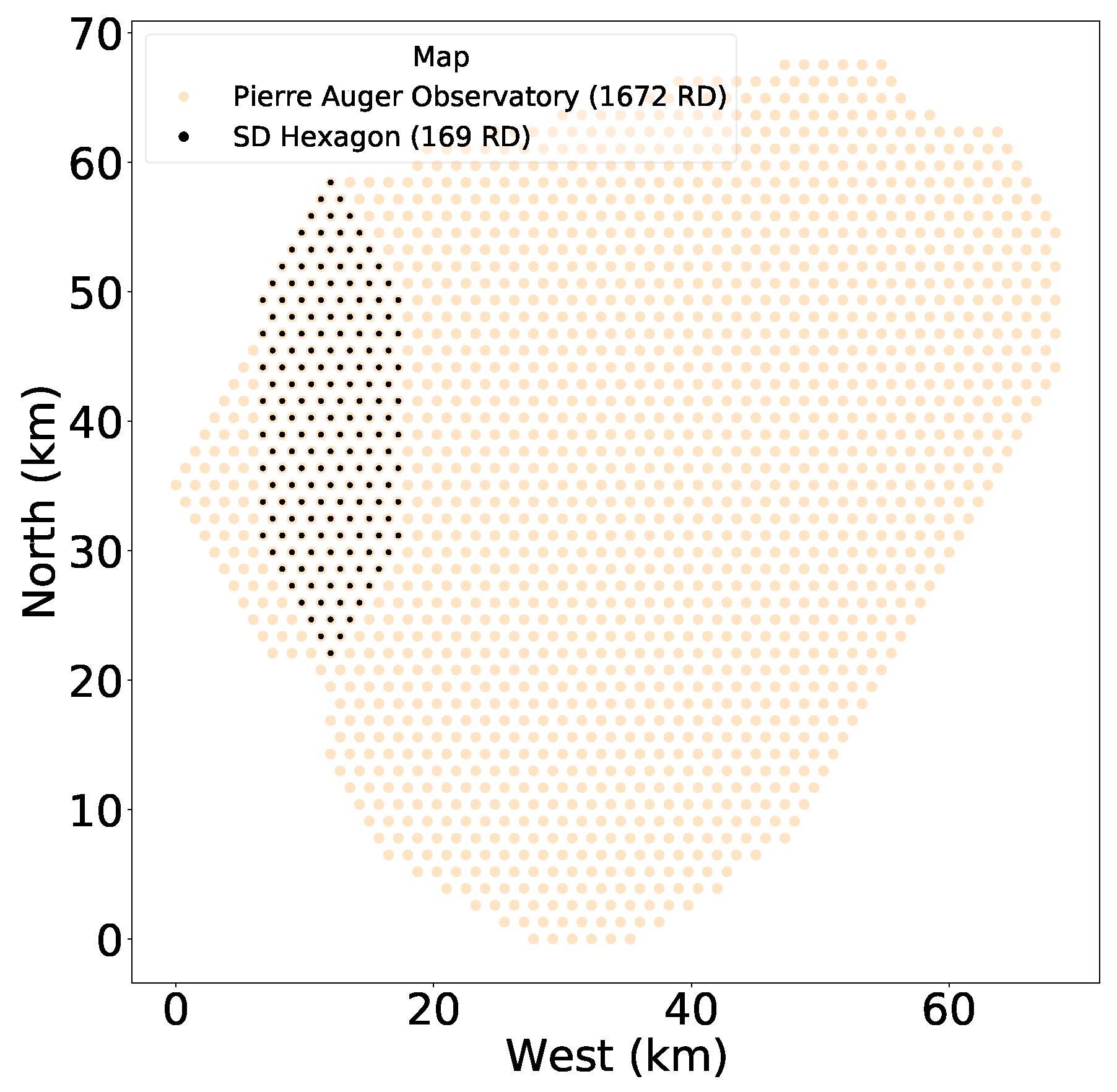
We first conducted a preliminary radio emission study on inclined air showers with a smaller area of the full Pierre Auger Observatory, based on an elongated hexagonal map of surface detectors, called SD Hexagon (Figure 3).

The following CORSIKA models were used for the air shower simulations: QGSJETII-04 [24] as the high-energy hadronic interaction model, UrQMD [25] as the low-energy hadronic interaction model, including the CoREAS option to simulate radio emission with an optimized thinning of ${10}^{-6}$ and maximum weights. A sample of events was simulated for proton and iron as primary cosmic ray particles, with an optimum energy of $5\times {10}^{18}$ eV (i.e., the higher energy threshold of full detection efficiency for the Pierre Auger Observatory is around $3\times {10}^{18}$ eV, independently of the mass of the primary particle [5,9]), for different inclined air shower geometries defined by the zenith (from 60° to 85°, in steps of 5°) and azimuth (from 0° to 315°, in steps of 45°) angles. The shower core was fixed in the middle of the detector map. This resulted in a total of 48 simulated showers (for the SD Hexagon map) per primary particle, consisting of six zenith angles and eight azimuth angles per zenith. The detector location in the simulations is representative for the Pierre Auger Observatory, meaning that the input cards make use of its corresponding height above sea level (i.e., 1400 m), the Earth’s magnetic field, and atmospheric model (i.e., October in Malargüe).

The simulated raw electric field registered in the time domain for each radio antenna is further processed. It is filtered in the 30–80 MHz frequency band, at which the radio antennas of the Pierre Auger Observatory are sensitive. Subsequently, the SNR is extracted for each polarization channel (east–west, north–south, and vertical), along with the absolute SNR (the magnitude of the SNR for each polarization channel), using the REASPlot software tool, part of the REAS3 package [26]. We define a radio antenna with a strong registered signal as one that has an absolute SNR ≥ 2. The SNR provides information on how well we can distinguish the signal from the noise (It should be noted that it does not provide information about the signal’s quality or quantity. For this purpose, other properties are used, such as the electric field strength, in $\mathsf{\mu }$${\mathrm{Vm}}^{-1}$, or energy fluence, in eV${\mathrm{m}}^{-2}$).

We further analyze each simulation of the SD Hexagon map to determine the optimal scaling factor for the Cherenkov ellipse per primary particle (proton and iron). By scaling both its axes with this factor (referred to as the Cherenkov scalar), we define the resulting Cherenkov selection ellipse, which should ideally include all radio antennas with a SNR ≥ 2 (strong signal), and exclude all antennas with SNR < 2 (weak signal). In practice, however, errors can occur, namely antennas with weak signals may fall inside the selection ellipse, and those with strong signals may fall outside. The goal is to minimize the number of these misclassifications. We thus distinguish four classes of antennas, as follows:

• True Positives (TP): Antennas with strong signal inside the selection ellipse;
• False Positives (FP): Antennas with weak signal inside the selection ellipse;
• False Negatives (FN): Antennas with strong signal outside the selection ellipse;
• True Negatives (TN): Antennas with weak signal outside the selection ellipse.

This classification allows us to assign a score for each selection ellipse, based on the following evaluation metrics, listed in order of importance.

• Missed Candidate Antennas Ratio (MCAR). This metric quantifies the proportion of antennas with strong signal that are not included by the selection algorithm in the list of selected candidates (Equation (4)). It is particularly useful for ensuring that all relevant candidate antennas are included, as minimizing FN is more important than minimizing FP in this context, while additional FP antennas only increase simulation time, FN antennas can result in quality signal loss and negatively affect subsequent Monte Carlo analysis. MCAR ranges from 0 to 1, where 0 indicates perfect selection (no missed candidate antennas), and 1 means that all relevant antennas were excluded.

  $$\mathrm{MCAR}={\displaystyle \frac{\mathrm{FN}}{\mathrm{TP}+\mathrm{FN}}}$$

  (4)
• Matthews correlation coefficient (MCC). Recognized as one of the best general binary classification metrics, the MCC considers all four classes in its calculation (Equation (5)). It has a range from −1 to 1, where 1 indicates perfect prediction, 0 indicates randomness, and −1 indicates total disagreement between predictions and reality.

  $$\mathrm{MCC}={\displaystyle \frac{\mathrm{TP}\times \mathrm{TN}-\mathrm{FP}\times \mathrm{FN}}{\sqrt{(\mathrm{TP}+\mathrm{FP})(\mathrm{TP}+\mathrm{FN})(\mathrm{TN}+\mathrm{FP})(\mathrm{TN}+\mathrm{FN})}}}$$

  (5)
• ${\mathrm{F}}_1–\mathrm{score}$. A widely used metric in binary classification that ranges from 0 (poor performance) to 1 (perfect performance). However, it does not take into account the TN class (Equation (6)).

  $${\mathrm{F}}_1–\mathrm{score}={\displaystyle \frac{2\times \mathrm{TP}}{2\times \mathrm{TP}+\mathrm{FP}+\mathrm{FN}}}$$

  (6)
• Accuracy. It becomes less useful with imbalanced datasets, where the FP and FN classes are much smaller compared to the TP and TN classes (Equation (7)), as is the case in our dataset. It ranges from 0 (poor performance) to 1 (perfect performance).

  $$\mathrm{Accuracy}={\displaystyle \frac{\mathrm{TP}+\mathrm{TN}}{\mathrm{TP}+\mathrm{TN}+\mathrm{FP}+\mathrm{FN}}}$$

  (7)

To determine the optimal Cherenkov scalar, we tested values from 1 to 5, in steps of 0.1, for each simulation on the SD Hexagon map that meets the validity condition, i.e., having at least three radio antennas with strong registered signal. For all scalars in this range, we calculated the MCAR, MCC, ${\mathrm{F}}_1–\mathrm{score}$, and Accuracy of their corresponding Cherenkov selection ellipse. We then ranked all scalars based on their associated ellipse scores, using a priority rule in which MCAR is the most important metric, followed by the MCC, ${\mathrm{F}}_1–\mathrm{score}$, and then Accuracy. This means that in cases where two Cherenkov scalars have the same MCAR score, the ranking is determined next by comparing their MCC values. If those are also equal, the ${\mathrm{F}}_1–\mathrm{score}$ is used, and finally, Accuracy is considered as the last tie-breaker.

The results are displayed in

Table 1. Best Cherenkov scalar ranges for different zenith (rows) and azimuth (columns) angles of the SD Hexagon simulations for proton.

Angle	0°	45°	90°	135°	180°	225°	270°	315°
60°	N/A	N/A	N/A	N/A	N/A	N/A	N/A	N/A
65°	2.5–4.8	2.7–4.2	N/A	N/A	2.4–4.7	2.8–4.3	N/A	2.8–4.3
70°	2.9–3.6	1.8–3.0	2.6–4.2	3.1	3.0–3.7	3.1	2.5–4.1	3.1
75°	2.7–2.8	2.9	2.7–2.9	2.9	2.9–3.2	2.8	2.8–3.0	2.9
80°	2.1–3.4	2.5–2.7	2.4–2.6	2.5–2.7	2.1–3.3	2.5–2.7	2.9	2.5–2.7
85°	1.9–2.7	2.3	2.3–2.6	2.2	1.9–2.7	2.2	2.3–2.6	2.3

and

Table 2. Same as Table 1, for iron.

Angle	0°	45°	90°	135°	180°	225°	270°	315°
60°	N/A	N/A	N/A	N/A	N/A	N/A	N/A	N/A
65°	2.3–4.4	2.6–4.1	N/A	2.7–4.1	2.4–4.5	2.7–4.1	N/A	2.6–4.0
70°	2.9–3.6	3.0	2.5–4.0	3.0	2.9–3.6	3.0	2.5–4.1	3.0
75°	2.9–3.2	2.8	2.7–2.9	2.8	2.8–3.1	2.8	2.7–2.9	2.8
80°	2.1–3.3	2.5–2.7	2.4–2.6	2.5–2.7	2.1–3.3	2.5–2.7	2.8–2.9	2.5–2.7
85°	1.9–2.7	2.2	2.3–2.6	2.3	1.9–2.7	2.2	2.3–2.6	2.2

, which show the best scalar range for each simulation (a range is used when there is no difference between the values of the four evaluation metrics), per primary particle (proton and iron). An N/A value indicates that the simulation did not meet the validity condition.

Table 3. Best evaluation metric values for each zenith, averaged over all azimuth angles for proton.

Metric	MCAR	MCC	${\mathbf{F}}_1–\mathbf{Score}$	Accuracy
60°	N/A	N/A	N/A	N/A
65°	N/A	N/A	N/A	N/A
70°	0	0.92	0.92	0.99
75°	0	0.95	0.95	0.99
80°	0	0.98	0.98	0.99
85°	0	0.98	0.99	0.99

and

Table 4. Same as Table 3, for iron.

Metric	MCAR	MCC	${\mathbf{F}}_1–\mathbf{Score}$	Accuracy
60°	N/A	N/A	N/A	N/A
65°	N/A	N/A	N/A	N/A
70°	0	0.94	0.94	1
75°	0	0.94	0.94	0.99
80°	0	0.97	0.98	0.99
85°	0	0.97	0.99	0.98

present, for each zenith angle, the average of the best metric values across all azimuth angles. For each zenith-azimuth configuration, the best metric value is taken from the Cherenkov scalar range that performed the best, according to Table 1 and Table 2. If at least one simulation for a given zenith angle did not meet the validity condition, all metrics for that zenith are marked as N/A.

We observe that the distance between adjacent radio antennas at the Pierre Auger Observatory is favorable to detect air showers with zenith angles greater than 70° (very inclined air showers). For example, at 60°, only the station that overlaps the shower core records a strong electric field, and at 65°, the geomagnetic effect is observed (showers arriving from the north direction, i.e., azimuth 90°, are almost parallel to the magnetic field at the experiment location [27]) resulting in weak registered radio signals.

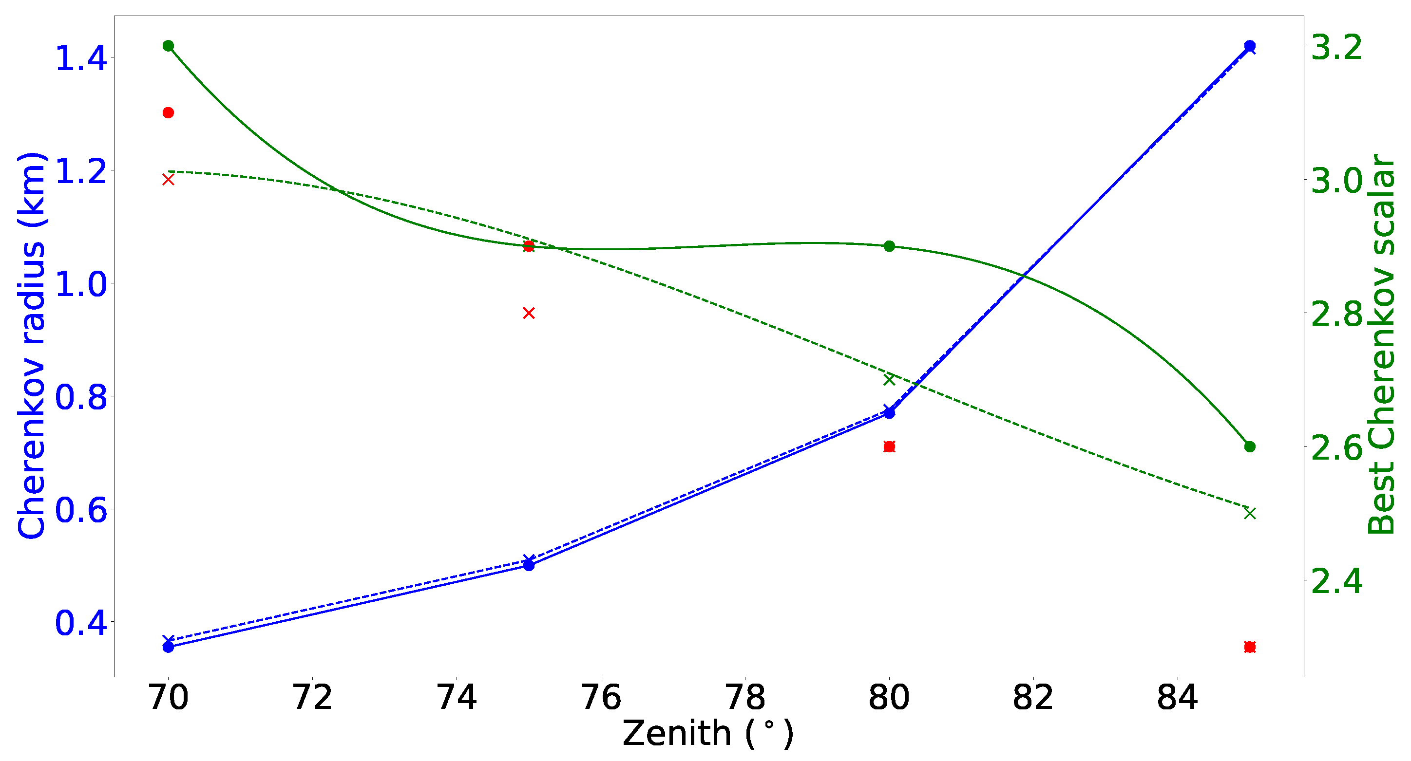
The Cherenkov radius (semi-minor axis) increases significantly with the zenith angle (Figure 4, blue), as the projected radio signal on the ground takes the form of an elongated ellipse. Regarding the iron simulations, there is not much difference from the proton, since the mean Xmax of the 48 iron simulated events is close to the one for proton. The higher the zenith angle, the narrower the range of possible Cherenkov scalar values (Figure 4, green).

We should take into account that for air showers with zenith angles greater than 80°, the SD Hexagon map becomes less efficient for air showers arriving from the east–west directions. This is due to the elongated shape of the hexagonal array along the north–south axis, which limits our ability to determine the full extent of the electric field strength in the east–west direction. The same limitation of the SD Hexagon map applies for zenith angles greater than 85°, regardless of the azimuth angle.

We further extracted from Table 1, for each zenith angle starting with 70°, the scalar value (or the scalar range, if multiple scalars had the same frequency) that appeared the most frequently across all azimuth angles (Figure 4, red). In cases where a range was selected, we further reduced it to a number by selecting the largest scalar of the range. These values will be used to predict candidate antennas expected to record strong signals, based on the zenith angle of the simulated air shower. A point to note is that the algorithm that calculates the Cherenkov radius requires the simulation’s output value of the distance from the shower core to X_max. This poses a challenge, as we do not know the slant depth of X_max before running the simulation. Therefore, we used a constant value for the slant depth of X_max of 750 g/cm²—value estimated by the QGSJETII-04 model for a proton UHECR at $5\times {10}^{18}$ eV. This value is also close to the mean X_max of 758.54 g/cm² from our 48 simulated events for proton, while the mean Xmax for iron simulations is 674.33 g/cm².

To evaluate the prediction, a Cherenkov scalar value of 4 was selected for simulations of very inclined air showers on the full array, ensuring that noisy radio antennas are also included. The simulations use the ideal map of the Pierre Auger Observatory, which has no gaps in the detector layout (Figure 3). In an optimal approach, proton and iron UHECRs with an energy of $5\times {10}^{18}$ eV are simulated for different geometries of the induced air showers defined by zenith angles ranging from 70° to 85°, in steps of 5°, and azimuth angles from 0° to 315°, in steps of 45°. This results in a sample dataset of 32 simulations per primary particle. The same full azimuth range in steps of 45 degrees is used for convenience in an optimal consideration of the full geometry of simulated showers.

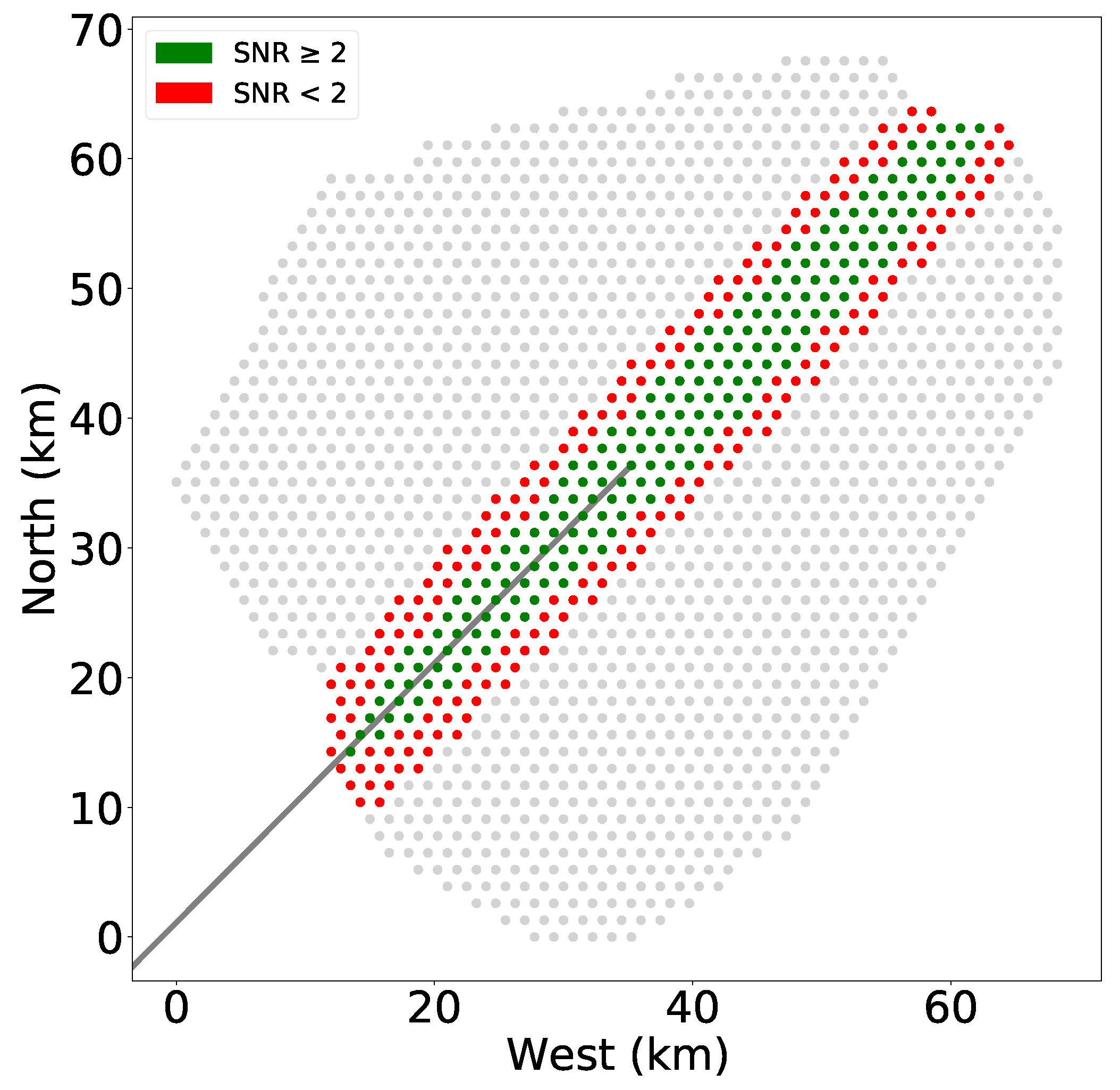
We calculated the centroid of the map as the average position of the antennas in both the north–south and east–west directions. Outliers—defined as antennas lying more than two standard deviations from the mean—were excluded from this calculation. The antenna nearest to this centroid was then selected to serve as the shower core position, allowing us to capture the electric field strength at the core. Using a Cherenkov scalar value of 4 (which includes noisy antennas for the purpose of validating the prediction) and rotated counterclockwise by the azimuth angle, the Cherenkov selection ellipse was applied to predict candidate antennas and generate the corresponding input cards for the simulations. An example of applying the selection algorithm and the simulated radio response of the selected candidate antennas with SNR ≥ 2 is shown in Figure 5.

The same algorithm was applied—using an upper limit of the Cherenkov scalar set to 4, instead of 5—to identify the optimal Cherenkov scalar range for each simulation per primary particle (

Table 5. Best Cherenkov scalar ranges for different zenith (rows) and azimuth (columns) angles of the ideal Auger map simulations for proton.

Angle	0°	45°	90°	135°	180°	225°	270°	315°
70°	3.1–3.9	1.9–3.2	2.6–4.0	3.2	3.0–3.8	3.2	2.8–4.0	1.9–3.1
75°	2.7–2.8	2.9	2.8–3.0	2.9	2.7–2.8	2.9	2.8–3.0	2.9
80°	2.9–3.0	2.5–2.7	2.4–2.6	2.8	2.9–3.0	2.8	2.9	2.8
85°	2.6	2.4	2.5	2.5	2.6	2.6	2.6	2.6

and

Table 6. Same as Table 5, for iron.

Angle	0°	45°	90°	135°	180°	225°	270°	315°
70°	2.9–3.6	3.0	2.5–4.0	3.0	2.9–3.6	3.0	2.5–4.0	3.0
75°	2.9–3.0	2.9	2.7–2.9	2.8	2.9–3.0	2.8	2.7–2.9	2.8
80°	2.8–3.0	2.5–2.7	2.4–2.6	2.5–2.7	2.8–3.0	2.5–2.7	2.7	2.5–2.7
85°	2.5	2.3	2.4	2.4	2.5	2.5	2.4	2.5

). Then, the most common range was extracted for each zenith angle across all azimuth angles, and the best metric values (

Table 7. Best evaluation metric values for each zenith, averaged over all azimuth angles, of the ideal Auger map simulations for proton.

Metric	MCAR	MCC	${\mathbf{F}}_1–\mathbf{Score}$	Accuracy
70°	0	N/A	0.92	0.91
75°	0	0.93	0.96	0.96
80°	0	0.91	0.94	0.96
85°	0	0.84	0.92	0.92

and

Table 8. Same as Table 7, for iron.

Metric	MCAR	MCC	${\mathbf{F}}_1–\mathbf{Score}$	Accuracy
70°	0	N/A	0.94	0.95
75°	0	0.89	0.94	0.94
80°	0	0.93	0.96	0.97
85°	0	0.86	0.93	0.93

), as we did for the SD Hexagon analysis. A value of N/A in Table 7 and Table 8 indicates that at least one simulation at a given zenith angle (in this case 70°) involved two or more antenna classes for which the sum in the MCC denominator was zero, making the MCC undefined due to division by zero.

Compared with the predicted values from the SD Hexagon simulations (

Table 9. Actual versus predicted best Cherenkov scalars for each zenith angle of the full ideal Auger map simulations for proton (p) and iron (Fe).

Zenith Angle	Actual Best Scalars (p|Fe)	Predicted Best Scalars (p|Fe)
70°	3.2|3.0	3.1|3.0
75°	2.9|2.8–2.9	2.9|2.8
80°	2.8–2.9|2.5–2.7	2.6|2.6
85°	2.6|2.5	2.3|2.3

, column 3), where the predictions are accurate and comparable between the proton and iron simulations, for zenith angles > 80°, the actual best scalars of both proton and iron are slightly larger than predicted (Table 9, column 2). The discrepancy is likely due to the usage of MCAR as the primary evaluation metric, which gives more importance to the FN class by making sure that all candidate antennas are selected, thus resulting in a MCAR of 0. It thus confirmed the limitation of the SD Hexagon map in terms of less efficiency for showers arriving from the east–west directions, due to its elongated shape area along the north–south direction.

By extracting the biggest values from the optimal scalar ranges, we model the relationship between the zenith angle and the best Cherenkov scalar for that zenith using a third-degree (cubic) polynomial. The fitting was performed using Python’s numpy.polyfit function with degree 3, which minimizes the least squares error between the predicted and observed values. The resulting fitted Equations (8) and (9) for the optimal Cherenkov scalar as a function of the zenith angle ($\theta$/degree) for inclined air showers, per primary particle (p and Fe), are the following:

$$\mathit{\text{Optimal Cherenkov scalar}}\left(\mathit{p}\right)=-0.0008\times {\theta }^3+0.186\times {\theta }^2-14.41\times \theta +374.9$$

(8)

$$\mathit{\text{Optimal Cherenkov scalar}}\left(\mathit{Fe}\right)=0.0001333\times {\theta }^3-0.032\times {\theta }^2+2.517\times \theta -62.1$$

(9)

However, since the fits were made for higher zenith angles, i.e., between 70 and 85 degrees, these optimal Cherenkov scalars per primary type (proton and iron) represent the validity range of the given Equations (8) and (9). Therefore, for lower zenith angles, i.e., below 70 degrees, the factor of 4 should be used instead.

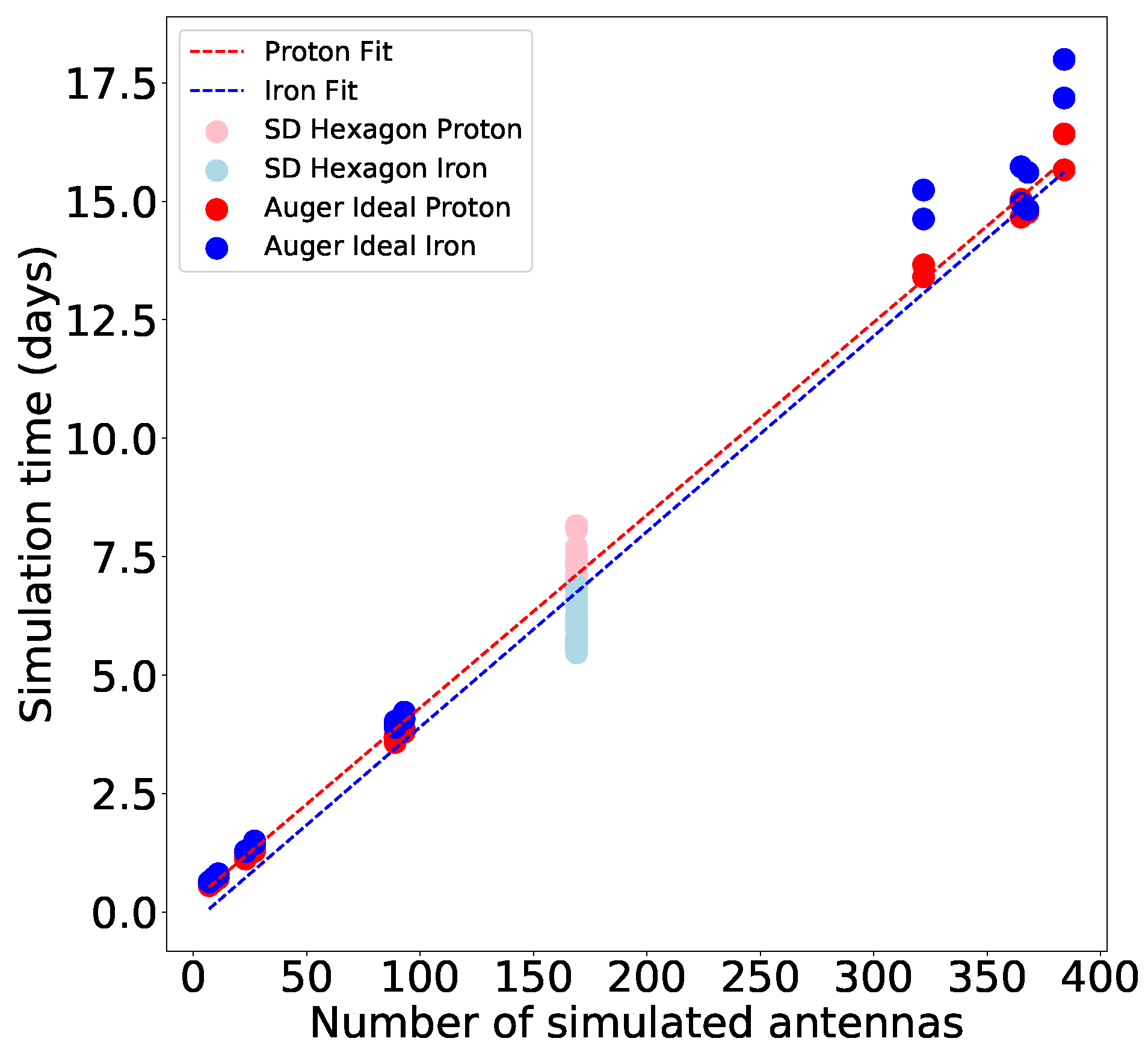
Because the primary goal of this selection is time efficiency, we aimed to evaluate how much time was saved. To do so, we extracted the simulation time for each individual run. To improve the accuracy of our estimation, each of the 32 simulations using the ideal Auger map was repeated three times for proton, and the average runtime was calculated (Figure 6). By including both SD Hexagon simulations (with zenith angles greater than 70°) and ideal Auger map simulations, a comprehensive analysis was performed. First, the Pearson correlation coefficient indicates a very strong linear correlation for both proton and iron—close to 1—between the number of simulated antennas and the simulation time, which is also evident from Figure 6. Knowing this, we further perform a simple linear regression to model the simulation time as a linear function of the number of antennas, using LinearRegression from sklearn.linear_model, which minimizes the least squares error between predicted and observed values. The regressions fitted to all data points (Equations (10) and (11)) have a coefficient of determination $R^2=0.99$ for proton, and, respectively, $R^2=0.96$ for iron.

$$\mathit{\text{Simulation time}} (\mathit{p}/\mathit{days})=0.0407\times \mathit{\text{Number of antennas}}+0.242$$

(10)

$$\mathit{\text{Simulation time}} (\mathit{Fe}/\mathit{days})=0.0412\times \mathit{\text{Number of antennas}}-0.226$$

(11)

These linear functions predict that simulating an array of 1672 antennas—the full list of radio detectors on the ideal Auger map—would have taken nearly 68 days for both proton and iron showers, which is an enormous amount of time. Moreover, using the previously computed optimal Cherenkov scalar function, we can estimate how much time could have been saved if instead of using a constant scalar of 4, we would have used the optimal value. A smaller number of antennas would have resulted in a shorter simulation time. As a result,

Table 10. Reduction in time (%) per each ideal Auger map simulation (zenith-rows, azimuth-columns) when using the optimal Cherenkov scalar (p) function instead of a constant value of 4.

Angle	0°	45°	90°	135°	180°	225°	270°	315°
75°	36.42%	36.42%	45.78%	36.42%	36.42%	36.42%	45.78%	36.42%
80°	48.51%	45.39%	50.53%	45.39%	48.51%	45.39%	50.53%	45.39%
85°	43.32%	37.01%	40.88%	39.59%	43.32%	37.01%	40.88%	39.59%

and

Table 11. Same as Table 10, for iron.

Angle	0°	45°	90°	135°	180°	225°	270°	315°
75°	55.74%	55.74%	68.00%	55.74%	55.74%	55.74%	68.00%	55.74%
80°	59.41%	63.14%	61.69%	63.14%	59.41%	63.14%	61.69%	63.14%
85°	45.51%	40.57%	43.88%	42.65%	45.51%	40.57%	43.88%	42.65%

show, for each simulation per primary particle (p and Fe), the percentage reduction in simulation time, starting from zenith angle 75°. This angle is chosen because it is the lowest at which at least six antennas are simulated, i.e., the minimum number for which Equation (11) returns a positive value. The equation is most useful for cases in which several tens to hundreds of antennas are simulated. Furthermore, the reason we present the reduction in time as a percentage, instead of a raw value, is because even if different computer architectures may require different amounts of CPU time, the percentage reduction in time should remain consistent.

We observe that for highly inclined air showers, i.e., those with zenith angles above 75°, the use of the optimal Cherenkov scalar function would have saved several days of simulation time on our computer architecture. Furthermore, at the highest zenith angles (above 85°), the time savings could reach up to a full week or even more.

We should also note that the inverse of the optimal Cherenkov scalar function allows one to estimate the number of antennas required given a fixed time constraint. For example, if a simulation of a proton on the ideal Auger map must be completed within a maximum of one week, up to 166 antennas could be used (Figure 6, proton). Or, if we want to simulate an iron-induced inclined shower with a primary energy of $5\times {10}^{18}$ eV, and about 350 antennas, approximately 14 days of simulation time are needed (Equation (11)) on our computer architecture. The higher the zenith angle, as well as the heavier the primary nuclei, the longer the simulation time (Figure 6, iron).

3. Conclusions

We have implemented an optimal method for selecting candidate antennas with good registered radio signals from inclined EAS induced by protons and iron nuclei, applicable to any radio detector layout. The predicted reduced number of candidate observers drastically decreases the simulation time—by even more than 50% for the heaviest nuclei, at the highest zenith angles—making data analysis considerably more affordable. In the future, additional simulations at intermediate zenith angles will be necessary to evaluate how well the fitted equation aligns with the optimal Cherenkov scalar as a function of the zenith angle, as well as of primary heavy nuclei at higher energies to look for mass-sensitive discrepancies, if any. Furthermore, a scalability study using hybrid distributed-shared memory systems—such as parallelizing simulations with MPI (Message Passing Interface) for the distributed part and OpenMP/PThreads for the shared one—can be done to reduce even more the simulation time and obtain a significant performance speedup.

This study facilitates the increase in the statistics of simulated radio data for complementary and modern physics analysis, such as the machine learning algorithms applied to the data. It comes in support of further simulations for inclined air showers, with application at the Pierre Auger Observatory, or any other planned experiment in the future. The benefit of fast simulations of highly inclined and energetic air showers, initiated by either light or heavy nuclei, is essential for data analysis of polarized radio signals, such as Convolution Neural Network classification of simulated CoREAS events for inferring the nuclear mass of the primary cosmic ray particle.