Evolution of the Early Universe in Einstein–Cartan Theory

Abstract

Einstein–Cartan theory is a generalization of general relativity that introduces spacetime torsion. In this paper, we perform phase space analysis to investigate the evolution of the early universe in Einstein–Cartan theory. By studying the stability of critical points in the dynamical system, we find that there exist two stable critical points which represent an Einstein static solution and an expanding solution, respectively. After analyzing the phase diagram of the dynamical system, we find that the early universe may exhibit an Einstein static state, an oscillating state, or a bouncing state. By assuming the equation of state $\omega$ can decrease over time t, the universe can depart from the initial Einstein static state, oscillating state, or bouncing state and then evolve into an inflationary phase. Then, we analyze four different inflationary evolution cases in Einstein–Cartan theory and find that a time-variable equation of state $\omega$ cannot yield values of $n_s$ and r consistent with observations, while a time-invariant equation of state $\omega$ is supported by the Planck 2018 results. Thus, in Einstein–Cartan theory, the universe likely originates from a bouncing state rather than an Einstein static state or an oscillating state.

1. Introduction

Based on general relativity, the standard cosmological model was established and can be used to describe the evolution of the universe. Although the standard cosmological model has achieved great success, it implies that the universe originated from a big bang singularity. However, in general relativity, spacetime is considered as a Riemannian manifold with vanishing torsion and zero non-metricity. The generalization of general relativity in a spacetime with torsion is named Einstein–Cartan theory, where the torsion arises from the intrinsic spin of elementary particles. Since there is a relationship between the intrinsic spin of fermionic matter and spacetime torsion, spacetime torsion is not a dynamical quantity [1,2,3]. Thus, the spinor field can be incorporated into torsion-free general relativity [4], and Einstein–Cartan theory can be equivalent to general relativity with an effective perfect fluid in the energy-momentum tensor [5,6,7,8,9], which can behave as stiff matter with negative energy density in cosmology [10,11,12]. Since this negative energy density directly leads to gravitational repulsion, it became very significant in the early universe. Therefore, the big bang singularity in the standard cosmological model can be resolved in Einstein–Cartan theory through a nonsingular big bounce [13,14], leading to Einstein static universe [15] or emergent universe models [16]. Furthermore, the Einstein–Cartan theory not only can address the flatness and horizon problems without requiring inflation [17,18,19], but also leads to inflation [12] and late-time acceleration [20]. Recently, Einstein–Cartan theory has regained much attention and has been widely studied in inflationary models [21,22,23,24,25], preheating [26], quantum cosmology [27,28], gravitational waves [29,30,31,32], Hubble tension [33], Morris–Thorne wormhole [34], gravitational collapse [35], and other physical effects [36,37,38,39,40].

Phase space analysis is a dynamical method to analyze the qualitative behavior of a dynamical system. In this approach, critical points obtained from the solutions of the autonomous system can be used to describe the evolution of the system. The stable critical points are referred to as attractors, which describe the final state of the system. When applied to cosmology, it can be used to analyze the late-time evolution of the universe and has been extensively studied in many cosmological models, such as single scalar field models [41,42,43,44], $f\left(R\right)$ gravity [45], $f\left(T\right)$ theory [46,47], mimetic gravity [48], the Chaplygin model [49], holographic dark energy [50,51,52,53,54,55,56], and so on. Recently, phase space analysis has been extended to analyze the evolution of the early universe by defining some new dimensionless variables, which can describe the expansion or contraction of the universe [57]. So, can this method be used to answer the question of whether the early universe originated from an Einstein static state, an oscillating state, or a bouncing state within the framework of Einstein–Cartan theory?

Inflation is a period of exponential expansion before the radiation-dominated era in modern cosmology [58,59]. It not only addresses the challenges of the Big Bang cosmology but also explains the quantum origin of the Cosmic Microwave Background temperature anisotropies and the Large-Scale Structure [60,61,62]. During inflation, the small quantum fluctuations are amplified to physical scales and lead to nearly scale-invariant, Gaussian, and adiabatic primordial perturbations [63]. This information is encoded in the primordial scalar power spectrum, which is characterized by the scalar spectral index $n_s$ and constrained by the Planck 2018 results as $n_s=0.9668\pm 0.0037$ [64]. Based on the constraint on the scalar spectral index $n_s$, various inflation models have been proposed [65,66,67,68,69,70,71,72,73,74,75,76,77,78,79,80,81,82,83,84,85,86,87,88,89,90,91,92,93,94,95,96,97]. So, in the Einstein–Cartan theory, after the universe originates from an Einstein static state, an oscillating state, or a bouncing state and then evolves into the inflation era, can it yield $n_s$ consistent with observations?

This paper has two objectives: to examine which states may have existed in the early universe, and to analyze inflation under observational constraints in Einstein–Cartan theory. The paper is organized as follows. In Section 2, we briefly review the field equations in Einstein–Cartan theory. In Section 3, we analyze the evolution of the early universe in Einstein–Cartan theory. In Section 4, we analyze the inflation in Einstein–Cartan theory. Finally, our main conclusions are presented in Section 5.

2. Field Equation

In Einstein–Cartan theory, the field equation can be written as [7,12]

$$G^{\mu \nu }=\kappa {\tilde{T}}^{\mu \nu },$$

(1)

with

$${\tilde{T}}^{\mu \nu }=T^{\mu \nu }+{\theta }^{\mu \nu }=(\rho +p-{\rho }_s-p_s)u^{\mu }{u}^{\nu }-(p-p_s)g^{\mu \nu },$$

(2)

and

$${\rho }_s=p_s={\displaystyle \frac{\kappa }{4}}{\sigma }^2.$$

(3)

Here, $u^{\mu }$ is the four-velocity, ${\sigma }^2$ represents the spin density scalar, and $\kappa =8\pi G$. Since $p_s={\rho }_s$, the effect of torsion and spin matter can be treated as stiff matter with negative energy density and pressure.

To study the evolution of the universe in Einstein–Cartan theory, we consider a homogeneous and isotropic universe described by the Friedman–Lema$\widehat{i}$tre–Robertson–Walker (FLRW) spacetime with the metric

$$d{s}^2=d{t}^2-a^2\left(t\right)\left[{\displaystyle \frac{d{r}^2}{1-k{r}^2}}+r^2(d{\theta }^2+{sin}^2\theta d{\varphi }^2)\right],$$

(4)

where t is the cosmic time, $a\left(t\right)$ represents the cosmic scale factor, and $k=0, 1, -1$ denote a spatially flat, closed, or open universe, respectively. Then, substituting the metric into the field Equation (1), we obtain the $\left(00\right)$ and $\left(ii\right)$ components of Equation (1):

$$\begin{array}{ccc}& & H^2+{\displaystyle \frac{k}{a^2}}={\displaystyle \frac{\kappa }{3}}(\rho -{\rho }_s),\hfill \end{array}$$

(5)

$$\begin{array}{ccc}& & 2\dot{H}+3H^2+{\displaystyle \frac{k}{a^2}}=-\kappa (p-p_s),\hfill \end{array}$$

(6)

in which $\rho ={\displaystyle \frac{1}{2}}{\dot{\varphi }}^2+V$ and $p={\displaystyle \frac{1}{2}}{\dot{\varphi }}^2-V$ are the energy density and the pressure of the scalar field $\varphi$, and $\rho$ and ${\rho }_s$ satisfy the continuity equations

$$\dot{\rho }+3H(1+\omega )\rho =0,\dot{{\rho }_s}+6H{\rho }_s=0.$$

(7)

Here, $\omega$ is the equation of state and satisfies $-1\le \omega \le 1$.

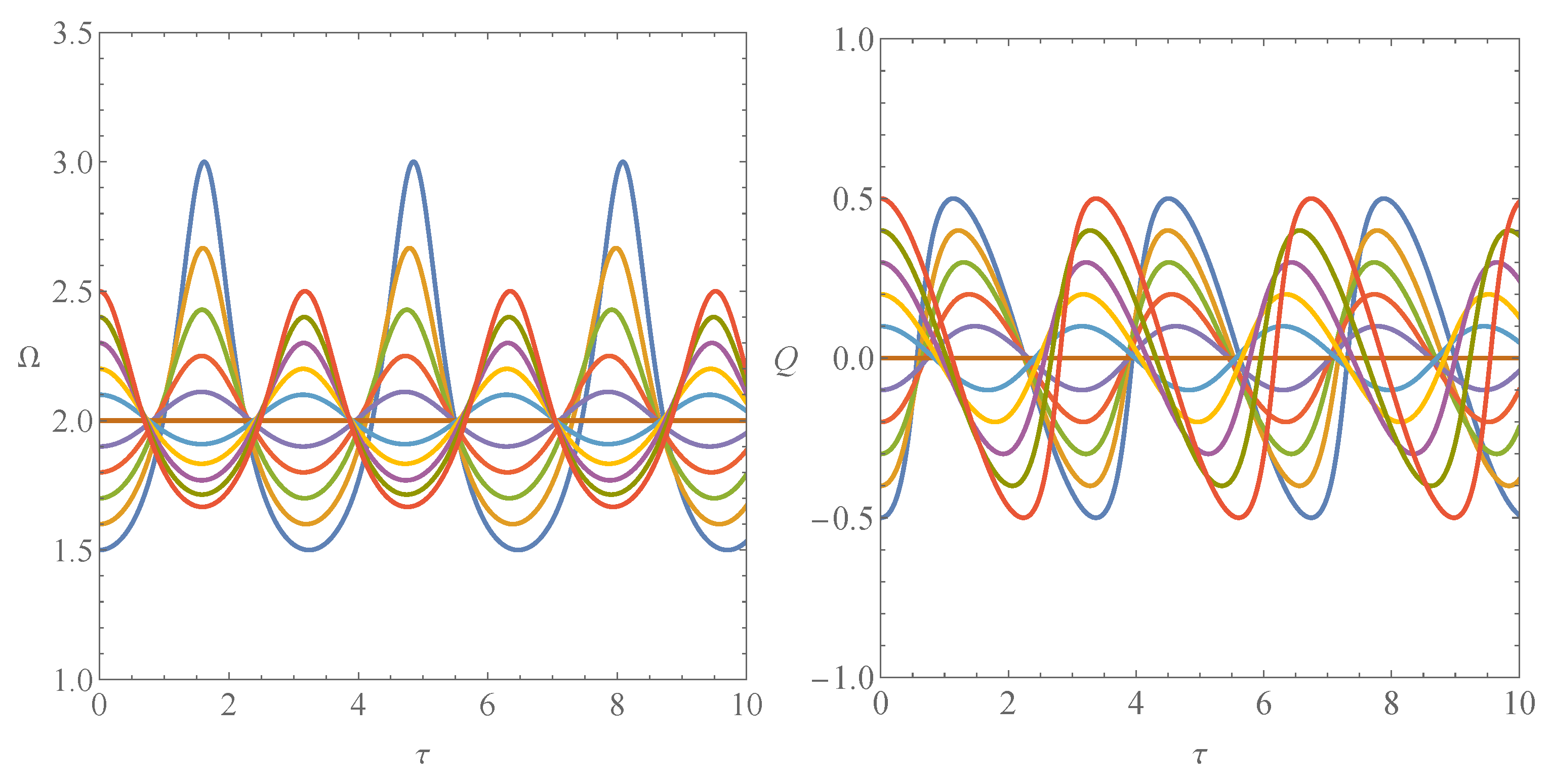
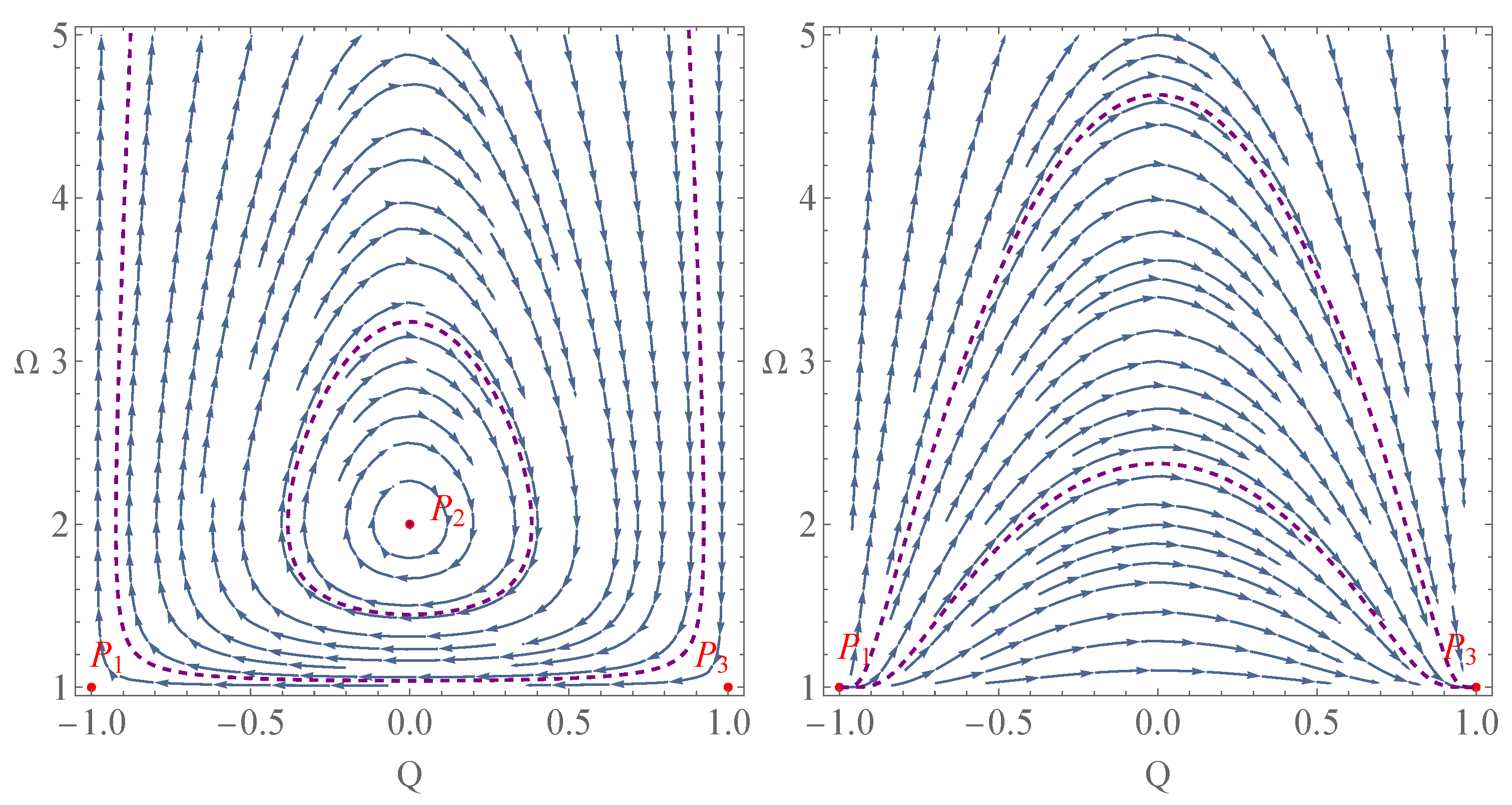
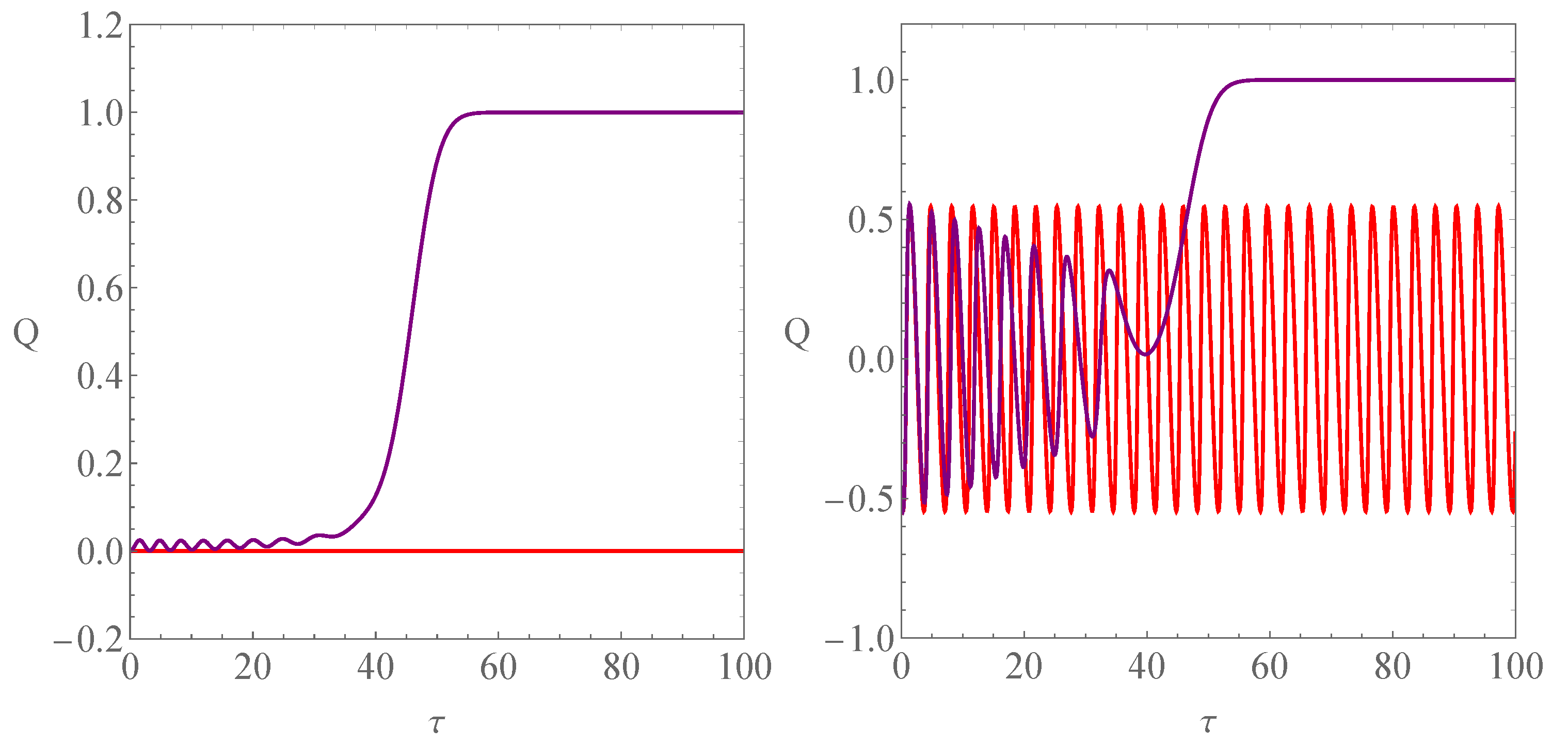
3. Phase Space Analysis

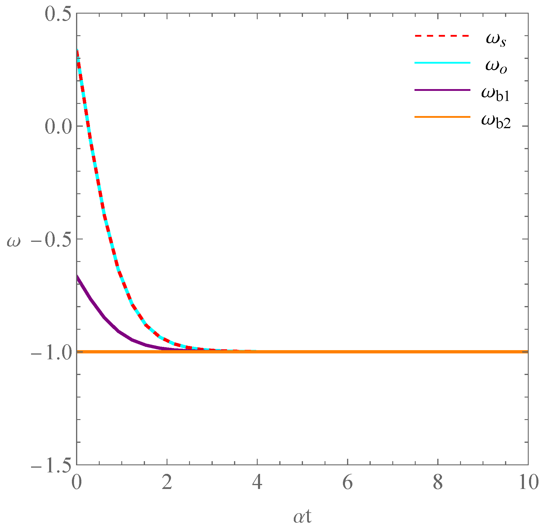
To analyze the dynamical evolution of the universe, we introduce the following dimensionless variables [57]:

$$\mathrm{\Omega }={\displaystyle \frac{\kappa }{3}}{R}^2\rho ,{\mathrm{\Omega }}_s={\displaystyle \frac{\kappa }{3}}{R}^2{\rho }_s,{\mathrm{\Omega }}_k={\displaystyle \frac{k{R}^2}{a^2}},Q=RH,$$

(8)

where R is the apparent horizon radius for the FLRW universe and it has the form

$$R=ar={\displaystyle \frac{1}{\sqrt{H^2+\frac{k}{a^2}}}}.$$

(9)

Using the dimensionless variables given in (8), the apparent horizon radius yields the relation

$$Q^2+{\mathrm{\Omega }}_k=1,$$

(10)

and the Friedmann Equation (5) can be written as

$$Q^2+{\mathrm{\Omega }}_k=\mathrm{\Omega }-{\mathrm{\Omega }}_s,$$

(11)

with $-1\le Q\le 1$, $0\le {\mathrm{\Omega }}_k\le 1$, ${\mathrm{\Omega }}_s\ge 0$ and $\mathrm{\Omega }\ge 1$. By combining Equations (10) and (11), we obtain ${\mathrm{\Omega }}_s=\mathrm{\Omega }-1$, showing that only one independent variable exists between $\mathrm{\Omega }$ and ${\mathrm{\Omega }}_s$. Then, introducing the time derivative

$$f^{\prime }={\displaystyle \frac{df}{d\tau }}=R\dot{f},$$

(12)

we obtain the dynamical system

$$\begin{array}{ccc}& & {\mathrm{\Omega }}^{\prime }=3(1-\omega )(1-\mathrm{\Omega })Q\mathrm{\Omega },\hfill \end{array}$$

(13)

$$\begin{array}{ccc}& & Q^{\prime }={\displaystyle \frac{1}{2}}(1-Q^2)[3(1-\omega )\mathrm{\Omega }-4],\hfill \end{array}$$

(14)

defined on the phase plane with $\mathrm{\Omega }\ge 1$ and $-1\le Q\le 1$. Now, we will analyze the phase space behavior of the dynamical system (13) and (14). The critical points of the autonomous system can be obtained by setting

$${\mathrm{\Omega }}^{\prime }=Q^{\prime }=0.$$

(15)

Then, we obtain five critical points. Since the existence conditions of these critical points are limited by $\mathrm{\Omega }\ge 1$, $-1\le Q\le 1$, and ${\mathrm{\Omega }}_s\ge 0$, two critical points are abandoned because ${\mathrm{\Omega }}_s=-1$. The remaining three critical points $(P_1,P_2,P_3)$ are shown in

Table 1. Critical points and their stability conditions.

$\mathit{Label}$	$(\mathbf{\Omega },\mathit{Q})$	${\mathbf{\Omega }}_{\mathit{s}}$	Existence	$\mathit{Eigenvalues}$	Conditions	$\mathit{Points}$
$P_1$	$(1,-1)$	0	$Always$	$-1-3\omega ,3-3\omega$	$-{\displaystyle \frac{1}{3}}<\omega <1$	$Saddlepoint$
					$-1\le \omega <-{\displaystyle \frac{1}{3}}$	$Unstablepoint$
$P_2$	$({\displaystyle \frac{4}{3(1-\omega )}},0)$	${\displaystyle \frac{1+3\omega }{3(1-\omega )}}$	$-{\displaystyle \frac{1}{3}}\le \omega <1$	$-\sqrt{2(-1-3\omega )},\sqrt{2(-1-3\omega )}$	$-{\displaystyle \frac{1}{3}}<\omega <1$	$Centerpoint$
$P_3$	$(1,1)$	0	$Always$	$1+3\omega ,-3+3\omega$	$-{\displaystyle \frac{1}{3}}<\omega <1$	$Saddlepoint$
					$-1\le \omega <-{\displaystyle \frac{1}{3}}$	$Stablepoint$

. From this table, we can see that $P_1$ is a contracting solution, $P_2$ denotes an Einstein static solution, and $P_3$ represents an expanding solution. The existence conditions show that $P_1$ and $P_3$ always exist, whereas $P_2$ is determined by the equation of state $\omega$.

To discuss the stability of the critical points, we will use the linear stability theory to analyze these points. By linearizing the autonomous system (13) and (14), we obtain two differential equations. The stabilities of these critical points are fully determined by the eigenvalues of the coefficient matrix of the two differential equations. If all eigenvalues of the critical point possess negative real parts, the point is stable; if all eigenvalues have a positive real part, the point is unstable; if at least two eigenvalues have real parts with opposite signs, this point is called a saddle point. In addition, if the eigenvalue has a zero real part, the critical point is called a non-hyperbolic point, for which the stability of the critical point cannot be determined by linear stability theory. To analyze the stability of the non-hyperbolic point, center manifold theory [53,98] or the numerical method [42,53,99,100] can be used.

After some calculations, we obtain the eigenvalues and stability conditions of these critical points, which are shown in Table 1. Specially, for the critical point $P_2$, the eigenvalues are purely imaginary, and this critical point is called a center, which is a stable point [101]. Projections of the time evolution of phase space trajectories for $P_2$ are shown in Figure 1, which indicates that a perturbation from the critical point will lead to an oscillation around this point rather than an exponential deviation. According to the results shown in Table 1, we can analyze the evolution of the early universe according to the equation of state $\omega$.

For $-{\displaystyle \frac{1}{3}}<\omega <1$, there are three critical points $P_1$, $P_2$, and $P_3$ in the autonomous system. $P_1$ denotes a saddle point corresponding to a contracting solution, $P_2$ denotes a stable Einstein static solution, and $P_3$ represents a saddle point corresponding to an expanding solution. In this case, the universe can become either an Einstein static universe or an oscillating universe. When $(\mathrm{\Omega },Q)$ takes the value of $P_2$, the early universe is an Einstein static state, while it becomes an oscillating state if $(\mathrm{\Omega },Q)$ takes other values. These cases are depicted in the left panel of Figure 2. In these figures, the red points denote the critical points, and the purple dashed lines represent an example of the evolutionary curves of the early universe.

For $-1\le \omega <-{\displaystyle \frac{1}{3}}$, the autonomous system has two critical points $P_1$ and $P_3$. $P_1$ denotes an unstable contracting solution, while $P_3$ denotes a stable expanding solution. Therefore, in this case, the universe will evolve from a contraction phase to an expanding phase, and it represents a bouncing universe, as shown in the right panel of Figure 2.

Thus, the evolution of the early universe in Einstein–Cartan theory is determined by the initial conditions and the equation of state $\omega$, and the initial state of the universe may be an Einstein static universe, an oscillating universe, or a bouncing universe. After the universe originates from one of these initial states, it can evolve into a subsequent inflation era since point $P_3$ is an attractor for $-1\le \omega <-{\displaystyle \frac{1}{3}}$.

In contrast to analyses of the Einstein static state in Refs. [15,16] where the static state requires $\dot{a}=\ddot{a}=0$, and investigations of the bouncing state in Refs. [13,14], which impose $\dot{a}=0$ at the bounce, our analysis adopts phase space analysis without invoking these conditions.

It is interesting to note that the stability conditions of $P_2$ have also been obtained in the Einstein static universe [15] and the emergent universe [16]. When the early universe is an Einstein static universe and $\omega$ decreases to less than $-{\displaystyle \frac{1}{3}}$, the stability condition of the Einstein static solution $P_2$ is broken, and $P_3$ becomes a stable point, acting as an attractor. As a result, the universe exits from the stable Einstein static state $P_2$ and evolves into an expanding state described by $P_3$. In the left panel of Figure 3, we have plotted this transition. In this figure, the red line denotes an Einstein static universe with $\omega ={\displaystyle \frac{1}{3}}$, $\mathrm{\Omega }=2$, and $Q=0$, while the purple line illustrates this transition by considering $\omega$ decreasing over time $\tau$. We can see that when $\tau$ increases to a critical value, the universe transitions from the Einstein static phase to an expanding phase with $Q=1$, which is depicted by $P_3$.

If the initial state of the universe is an oscillating universe and $\omega$ decreases to less than $-{\displaystyle \frac{1}{3}}$, breaking down the oscillating conditions, the universe can exit from the oscillating state and evolve into an expanding phase described by $P_3$. In the right panel of Figure 3, we have plotted this evolutionary process. In this figure, the red line denotes an oscillating universe with $\omega ={\displaystyle \frac{1}{3}}$, while the purple line represents the evolutionary curve with a time-variable $\omega$ that decreases with time $\tau$. We can see that when $\tau$ increases to a critical value, the universe departs from the oscillating phase and evolves into an expanding phase with $Q=1$.

4. Inflation

In Section 3, we find that in Einstein–Cartan theory, the early universe can originate from three different states: (i) an Einstein static state; (ii) an oscillating state; (iii) a bouncing state. After the universe originates from one of these initial states, it can evolve into a subsequent inflation era. In this section, we analyze the scalar spectral index $n_s$ and the tensor-to-scalar ratio r produced during the universe’s evolution from each of the three different initial states into the inflationary epoch, and then use Planck 2018 results to constrain them and discuss from which initial state the universe is likely to originate.

To analyze inflation in Einstein–Cartan theory, we ignore the role of spatial curvature k and the spin density scalar ${\sigma }^2$ in the Mukhanov–Sasaki equation and focus on their effect on the dynamical evolution process, as spacetime is nearly flat and the scale factor a is very large after inflation ends. Thus, the inflation is driven by the scalar field. Then, we adopt the slow-roll parameter ${ϵ}_n$, defined by the Hubble parameters H and its derivative $\dot{H}$, which are given as [102]

$${ϵ}_1=-{\displaystyle \frac{\dot{H}}{H^2}},{ϵ}_2={\displaystyle \frac{\dot{{ϵ}_1}}{H{ϵ}_1}}.$$

(16)

Combining Equations (5) and (6), we obtain

$$\dot{H}=-3H^2+{\displaystyle \frac{\kappa }{2}}(1-\omega )\rho -2{\displaystyle \frac{k}{a^2}}.$$

(17)

Using Equations (5) and (17), we can write the slow-roll parameters ${ϵ}_1$ and ${ϵ}_2$ as

$$\begin{array}{ccc}& & {ϵ}_1={\displaystyle \frac{6\frac{k}{a^2}+3\kappa [2{\rho }_s-(1+\omega )\rho ]}{6\frac{k}{a^2}+2\kappa ({\rho }_s-\rho )}},\hfill \end{array}$$

(18)

$$\begin{array}{ccc}& & {ϵ}_2={\displaystyle \frac{\kappa \left[{(1+3\omega )}^2\frac{k}{a^2}\rho +[-16\frac{k}{a^2}+3\kappa {(1-\omega )}^2\rho ]{\rho }_s\right]}{\left[3\frac{k}{a^2}+\kappa ({\rho }_s-\rho )\right]\left[2\frac{k}{a^2}+\kappa [2{\rho }_s-(1+\omega )\rho ]\right]}}.\hfill \end{array}$$

(19)

Now, utilizing the slow-roll parameters ${ϵ}_1$ and ${ϵ}_2$, we can calculate the scalar spectral index $n_s$ and the tensor-to-scalar ratio r using the following expressions [102]:

$$\begin{array}{ccc}& & n_s=1-2{ϵ}_1-2{ϵ}_2,\hfill \end{array}$$

(20)

$$\begin{array}{ccc}& & r=16{ϵ}_1.\hfill \end{array}$$

(21)

4.1. $k=0$

Considering the situation where the spacetime is nearly flat after inflation ends, we assume $k=0$, and Equation (18) provides the relation

$${\displaystyle \frac{{\rho }_s}{\rho }}=1-{\displaystyle \frac{3(1-\omega )}{2(3-{ϵ}_1)}}.$$

(22)

Then, using Equations (18)–(22), the scalar spectral index $n_s$ can be rewritten as

$$n_s=19-{\displaystyle \frac{3}{8}}r+6\omega -{\displaystyle \frac{288(1+\omega )}{r}},$$

(23)

In Figure 4, considering the constraint $n_s=0.9668\pm 0.0037$ for $r_{0.002}<0.058$ [64], we have plotted the relation between $n_s$ and $r_{0.002}$ for different $\omega$. This figure shows that to obtain $n_s$ and r supported by Planck 2018 results, the equation of state $\omega$ needs to approach $-1$ during inflation. It is worth noting that during slow-roll inflation in General Relativity, the equation of state parameter $\omega$ satisfies $\omega =-1+{\displaystyle \frac{2}{3}}{ϵ}_1$, which is approximately $-1$ as a result of ${\dot{\varphi }}^2\ll V$ [103]. Thus, the results shown in Figure 4 are consistent with the value of $\omega$ given by the slow-roll inflation in General Relativity.

4.2. $k=1$

In Section 3, we found that the early universe in Einstein–Cartan theory has three different origins: (i) Einstein static state; (ii) oscillating state; (iii) bouncing state. In this subsection, we will combine these results to analyze the inflation in the case $k=1$. For the case $k=1$, we cannot obtain the analytical expression for the relationship between $n_s$ and r. To analyze the inflation for $k=1$, we adopt a numerical method. We analyze four different inflationary evolution cases: (i) originating from an Einstein static state with a time-variable equation of state ${\omega }_s={\displaystyle \frac{1}{3}}[1-4{\omega }_{0}tanh\left(\alpha t\right)]$, and then evolving into the inflationary phase; (ii) originating from an oscillating state with a time-variable equation of state ${\omega }_o={\displaystyle \frac{1}{3}}[1-4{\omega }_{0}tanh\left(\alpha t\right)]$, and then evolving into the inflationary phase; (iii) originating from a bouncing state with a time-variable equation of state ${\omega }_{b1}=-{\displaystyle \frac{2}{3}}[1+{\displaystyle \frac{1}{2}}{\omega }_{0}tanh\left(\alpha t\right)]$, and then evolving into the inflationary phase; (iv) originating from a bouncing state with a time-invariant equation of state ${\omega }_{b2}=-{\omega }_0$, and then evolving into the inflationary phase. Parameter $\alpha$ has dimensions of inverse time, and ${\omega }_0$ is a value chosen based on the results in Figure 4. In Figure 5, we have plotted the evolutionary curves for these $\omega$. With the increase in $\alpha t$, all curves for $\omega$ approach $-{\omega }_0$, which corresponds to the equation of state during slow-roll inflation.

Combining Equations (5) and (6), we obtain the following equation by eliminating $\rho$:

$$2\dot{H}+3(\omega +1)H^2+(3\omega +1){\displaystyle \frac{1}{a^2}}=\kappa (1-\omega ){\rho }_s.$$

(24)

Solving this equation numerically for different $\omega$, respectively, we obtain different inflationary evolution curves, which are shown in Figure 6. The left panel of Figure 6 shows the evolutionary curves of the scale factor a over time $\alpha t$, while the right panel shows the evolutionary curves for the e-folds number N, which is defined as $N=ln{\displaystyle \frac{a}{a_0}}$. The red dashed line indicates that the universe originates from the Einstein static state and subsequently evolves into the inflationary phase as the equation of state ${\omega }_s$ decreases; the cyan line shows that the universe starts from an oscillating state and then transitions into the inflationary phase as the equation of state ${\omega }_o$ decreases; the purple line represents that the universe begins from a bouncing state and then evolves into the inflationary phase as the equation of state ${\omega }_{b1}$ decreases; the orange line denotes that the universe begins from a bouncing state and then evolves into the inflationary phase with a constant equation of state ${\omega }_{b2}$. From these figures, we can see that inflation can occur in all these cases, and the e-folds number N can exceed 65 as time increases. Additionally, the evolutionary curves for the universe originating from a static or oscillating state are nearly overlapping.

Then, by numerically solving Equation (24), we obtain the relation between the scalar spectral index $n_s$ (20) and the tensor-to-scalar ratio r (21) for different cases, as shown in Figure 7. In this figure, we overlay our numerical results with Planck 2018 results [64]. This figure shows that the time-variable equation of state $\omega$ cannot yield results consistent with the observations, while a time-invariant equation of state $\omega$ is supported by the Planck 2018 results, and that the scalar spectral index $n_s$ and tensor-to-scalar ratio r depend on both the initial state of the universe and the evolution of $\omega$ during the transition to inflation. Thus, in Einstein–Cartan theory, the universe is unlikely to originate from an Einstein static state or an oscillating state since subsequent inflation cannot yield $n_s$ and r consistent with the observations. Instead, the universe is likely to originate from a bouncing state with a time-invariant equation of state $\omega \approx -1$.

In Einstein–Cartan theory, the emergent universe cannot produce $n_s$ and r that are consistent with observations. An emergent universe, as supported by Planck 2018 results, may exist within various modified theories including scalar-tensor theory [104,105], mimetic gravity [106], non-minimal derivative coupling models [107,108], braneworld models [109], and f(R,T) gravity [110]. However, additional research is required to fully explore these possibilities.

5. Conclusions

Einstein–Cartan theory is a generalization of general relativity that introduces spacetime torsion, which can be equivalent to general relativity with an exotic stiff perfect fluid. In this paper, we analyze the evolution of the early universe in the Einstein–Cartan theory using the phase space analysis method. We find that there are three different critical points. The stability of these critical points is determined by the equation of state $\omega$. There exist two stable critical points $P_2$ and $P_3$. $P_3$ denotes an expanding solution and is stable for $-1\le \omega <-{\displaystyle \frac{1}{3}}$, while the stable Einstein static solution $P_2$ requires $-{\displaystyle \frac{1}{3}}<\omega <1$ and it is a center point. Therefore, $P_3$ can represent the final state of the evolution of the early universe. After analyzing the phase diagram of the dynamical system and considering different initial conditions and the equation of state $\omega$, we find there may exist an Einstein static universe, an oscillating universe, or a bouncing universe in the early universe. By assuming the equation of state $\omega$ can decrease over time t, the universe can depart from the initial Einstein static state, oscillating state, or bouncing state and then evolve into an inflationary state.

Subsequently, we analyze the inflation in Einstein–Cartan theory. For the spatial curvature $k=0$, we find that to obtain $n_s$ and r values supported by Planck 2018 results, the equation of state $\omega$ needs to approach $-1$ during inflation, and the value of $\omega$ is consistent with that given by the slow-roll inflation in General Relativity. For the spatial curvature $k=1$, we analyze four different inflationary evolution cases: (i) originating from an Einstein static state with a time-variable equation of state, and then evolving into the inflationary phase; (ii) originating from an oscillating state with a time-variable equation of state, and then evolving into the inflationary phase; (iii) originating from a bouncing state with a time-variable equation of state, and then evolving into the inflationary phase; (iv) originating from a bouncing state with a time-invariant equation of state, and then evolving into the inflationary phase. We find that the time-variable equation of state $\omega$ cannot yield results consistent with the observations, while a time-invariant equation of state $\omega$ is supported by the Planck 2018 results. Therefore, in Einstein–Cartan theory, the universe is unlikely to originate from an Einstein static state or an oscillating state; instead, it is likely to originate from a bouncing state with a time-invariant equation of state $\omega \approx -1$.

References

1. Hehl, F.; von der Heyde, P.; Kerlick, G.; Nester, J. General relativity with spin and torsion: Foundations and prospects. Rev. Mod. Phys. 1976, 48, 393. [Google Scholar] [CrossRef]
2. Hehl, F. On the kinematics of the torsion of space-time. Found. Phys. 1985, 15, 451. [Google Scholar] [CrossRef]
3. Hehl, F.; McCrea, J.; Mielke, E.; Neeman, Y. Metric-affine gauge theory of gravity: Field equations, noether identities, world spinors, and breaking of dilation invariance. Phys. Rep. 1995, 258, 1. [Google Scholar] [CrossRef]
4. Lledo, M.; Sommovigo, L. Torsion formulation of gravity. Class. Quantum Gravity 2010, 27, 065014. [Google Scholar] [CrossRef]
5. Weyssenhoff, J.; Raabe, A. Relativistic dynamics of spin-fluids and spin-particles. Acta Phys. Pol. 1947, 9, 7. [Google Scholar]
6. Obukhov, Y.; Korotky, V. The Weyssenhoff fluid in Einstein-Cartan theory. Class. Quantum Gravity 1987, 4, 1633. [Google Scholar] [CrossRef]
7. Smalley, L.; Krisch, J. Spinning fluid cosmologies in Einstein-Cartan theory. Class. Quantum Gravity 1994, 11, 2375. [Google Scholar] [CrossRef]
8. de Berredo-Peixoto, G.; De Freitas, E. On the cosmological effects of the Weyssenhoff spinning fluid in the Einstein-Cartan framework. Int. J. Mod. Phys. A 2009, 24, 1652. [Google Scholar] [CrossRef]
9. Vakili, B.; Jalalzadeh, S. Signature transition in Einstein-Cartan cosmology. Phys. Lett. B 2013, 726, 28. [Google Scholar] [CrossRef]
10. Hehl, F.; von der Heyde, P.; Kerlick, G. General relativity with spin and torsion and its deviations from Einstein’s theory. Phys. Rev. D 1974, 10, 1066. [Google Scholar] [CrossRef]
11. Nurgaliev, I.; Ponomariev, W. The earliest evolutionary stages of the universe and space-time torsion. Phys. Lett. 1983, 130B, 378. [Google Scholar] [CrossRef]
12. Gasperini, M. Spin-dominated inflation in the Einstein-Cartan theory. Phys. Rev. Lett. 1986, 56, 2873. [Google Scholar] [CrossRef] [PubMed]
13. Poplawski, N. Big bounce from spin and torsion. Gen. Relativ. Gravit. 2012, 44, 1007. [Google Scholar] [CrossRef]
14. Unger, G.; Poplawski, N. Big bounce and closed universe from spin and torsion. Astrophys. J. 2019, 870, 78. [Google Scholar] [CrossRef]
15. Atazadeh, K. Stability of the Einstein static universe in Einstein-Cartan theory. J. Cosmol. Astropart. Phys. 2014, 6, 020. [Google Scholar] [CrossRef]
16. Huang, Q.; Wu, P.; Yu, H. Emergent scenario in the Einstein-Cartan theory. Phys. Rev. D 2015, 91, 103502. [Google Scholar] [CrossRef]
17. Poplawski, N. Cosmology with torsion: An alternative to cosmic inflation. Phys. Lett. B 2010, 694, 181. [Google Scholar] [CrossRef]
18. Poplawski, N. Matter-antimatter asymmetry and dark matter from torsion. Phys. Rev. D 2011, 83, 084033. [Google Scholar] [CrossRef]
19. Poplawski, N. Nonsingular, big-bounce cosmology from spinor-torsion coupling. Phys. Rev. D 2012, 85, 107502. [Google Scholar] [CrossRef]
20. Shie, K.; Nester, J.; Yo, H. Torsion cosmology and the accelerating universe. Phys. Rev. D 2008, 78, 023522. [Google Scholar] [CrossRef]
21. Marco, A.; Orazi, E.; Pradisi, G. Einstein-Cartan pseudoscalaron inflation. Eur. Phys. J. C 2024, 84, 146. [Google Scholar] [CrossRef]
22. He, M.; Kamada, K.; Mukaida, K. Quantum corrections to Higgs inflation in Einstein-Cartan gravity. JHEP 2024, 1, 14. [Google Scholar] [CrossRef]
23. He, M.; Hong, M.; Mukaida, K. Starobinsky inflation and beyond in Einstein-Cartan gravity. J. Cosmol. Astropart. Phys. 2024, 5, 107. [Google Scholar] [CrossRef]
24. Piani, M.; Rubio, J. Higgs-Dilaton inflation in Einstein-Cartan gravity. J. Cosmol. Astropart. Phys. 2022, 5, 009. [Google Scholar] [CrossRef]
25. Shaposhnikov, M.; Shkerin, A.; Timiryasov, I.; Zell, S. Higgs inflation in Einstein-Cartan gravity. J. Cosmol. Astropart. Phys. 2021, 2, 008. [Google Scholar] [CrossRef]
26. Piani, M.; Rubio, J. Preheating in Einstein-Cartan Higgs Inflation: Oscillon formation. J. Cosmol. Astropart. Phys. 2023, 12, 002. [Google Scholar] [CrossRef]
27. Brandt, F.; Frenkel, J.; Martins-Filho, S.; McKeon, D. Quantization of Einstein-Cartan theory in the first order form. Ann. Phys. 2024, 462, 169607. [Google Scholar] [CrossRef]
28. Isichei, R.; Magueijo, J. Minisuperspace quantum cosmology from the Einstein-Cartan path integral. Phys. Rev. D 2023, 107, 023526. [Google Scholar] [CrossRef]
29. Ranjbar, M.; Akhshabi, S.; Shadmehri, M. Gravitational slip parameter and gravitational waves in Einstein-Cartan theory. Eur. Phys. J. C 2024, 84, 316. [Google Scholar] [CrossRef]
30. Elizalde, E.; Izaurieta, F.; Riveros, C.; Salgado, G.; Valdivia, O. Gravitational waves in Einstein-Cartan theory: On the effects of dark matter spin tensor. Phys. Dark Univ. 2023, 40, 101197. [Google Scholar] [CrossRef]
31. Battista, E.; De Falco, V. Gravitational waves at the first post-Newtonian order with the Weyssenhoff fluid in Einstein-Cartan theory. Eur. Phys. J. C 2022, 82, 628. [Google Scholar] [CrossRef] [PubMed]
32. Battista, E.; De Falco, V. First post-Newtonian generation of gravitational waves in Einstein-Cartan theory. Phys. Rev. D 2021, 104, 084067. [Google Scholar] [CrossRef]
33. Akhshabi, S.; Zamani, S. Cosmological distances and Hubble tension in Einstein-Cartan theory. Gen. Rel. Grav. 2023, 55, 102. [Google Scholar] [CrossRef]
34. Soni, S.; Khunt, A.; Hasmani, A. A study of Morris-Thorne wormhole in Einstein-Cartan theory. Int. J. Geom. Methods Mod. Phys. 2024, 21, 06. [Google Scholar] [CrossRef]
35. Hensh, S.; Liberati, S. Raychaudhuri equations and gravitational collapse in Einstein-Cartan theory. Phys. Rev. D 2021, 104, 084073. [Google Scholar] [CrossRef]
36. Costa, B.; Bonder, Y. Signature of Einstein-Cartan theory. Phys. Lett. B 2024, 849, 138431. [Google Scholar] [CrossRef]
37. Falco, V.; Battista, E.; Usseglio, D.; Capozziello, S. Radiative losses and radiation-reaction effects at the first post-Newtonian order in Einstein-Cartan theory. Eur. Phys. J. C 2024, 84, 137. [Google Scholar] [CrossRef]
38. Falco, V.; Battista, E. Analytical results for binary dynamics at the first post-Newtonian order in Einstein-Cartan theory with the Weyssenhoff fluid. Phys. Rev. D 2023, 108, 064032. [Google Scholar] [CrossRef]
39. Battista, E.; De Falco, V.; Usseglio, D. First post-Newtonian N-body problem in Einstein-Cartan theory with the Weyssenhoff fluid: Lagrangian and first integrals. Eur. Phys. J. C 2023, 83, 112. [Google Scholar] [CrossRef]
40. Bondarenko, S.; Pozdnyakov, S.; Zubkov, M. High energy scattering in Einstein-Cartan gravity. Eur. Phys. J. C 2021, 81, 613. [Google Scholar] [CrossRef]
41. Roy, N.; Banerjee, N. Dynamical systems study of Chameleon scalar field. Ann. Phys. 2015, 356, 452. [Google Scholar] [CrossRef]
42. Dutta, J.; Khyllep, W.; Tamanini, N. Cosmological dynamics of scalar fields with kinetic corrections: Beyond the exponential potential. Phys. Rev. D 2016, 93, 063004. [Google Scholar] [CrossRef]
43. Bhatia, A.; Sur, S. Dynamical system analysis of dark energy models in scalar coupled metric-torsion theories. Int. J. Mod. Phys. D 2017, 26, 1750149. [Google Scholar] [CrossRef]
44. Sola, J.; Gomez-Valent, A.; de Cruz Perez, J. Dynamical dark energy: Scalar fields and running vacuum. Mod. Phys. Lett. A 2017, 32, 1750054. [Google Scholar] [CrossRef]
45. Guo, J.; Frolov, A. Cosmological dynamics in f(R) gravity. Phys. Rev. D 2013, 88, 124036. [Google Scholar] [CrossRef]
46. Wu, P.; Yu, H. The dynamical behavior of f(T) theory. Phys. Lett. B 2010, 692, 176. [Google Scholar] [CrossRef]
47. Wei, H. Dynamics of Teleparallel Dark Energy. Phys. Lett. B 2012, 712, 430. [Google Scholar] [CrossRef]
48. Dutta, J.; Khyllep, W.; Saridakis, E.; Tamanini, N.; Vagnozzi, S. Cosmological dynamics of mimetic gravity. J. Cosmol. Astropart. Phys. 2018, 2, 041. [Google Scholar] [CrossRef]
49. Huang, Q.; Zhang, R.; Chen, J.; Huang, H.; Tu, F. Phase space analysis of the Umami Chaplygin model. Mod. Phys. Lett. A 2021, 36, 2150052. [Google Scholar] [CrossRef]
50. Setare, M.; Vagenas, E. The Cosmological dynamics of interacting holographic dark energy model. Int. J. Mod. Phys. D 2009, 18, 147. [Google Scholar] [CrossRef]
51. Banerjee, N.; Roy, N. Stability analysis of a holographic dark energy model. Gen. Relativ. Gravit. 2015, 47, 92. [Google Scholar] [CrossRef]
52. Huang, Q.; Huang, H.; Chen, J.; Zhang, L.; Tu, F. Stability analysis of a Tsallis holographic dark energy model. Class. Quantum Gravity 2019, 36, 175001. [Google Scholar] [CrossRef]
53. Bargach, A.; Bargach, F.; Ouali, T. Dynamical system approach of non-minimal coupling in holographic cosmology. Nucl. Phys. B 2019, 940, 10. [Google Scholar] [CrossRef]
54. Huang, Q.; Huang, H.; Xu, B.; Tu, F.; Chen, J. Dynamical analysis and statefinder of Barrow holographic dark energy. Eur. Phys. J. C 2021, 81, 686. [Google Scholar] [CrossRef]
55. Huang, H.; Huang, Q.; Zhang, R. Phase space analysis of Tsallis agegraphic dark energy. Gen. Relat. Gravit. 2021, 53, 63. [Google Scholar] [CrossRef]
56. Huang, H.; Huang, Q.; Zhang, R. Phase space analysis of barrow agegraphic dark energy. Universe 2022, 8, 467. [Google Scholar] [CrossRef]
57. Millano, A.; Jusufi, K.; Leon, G. Phase space analysis of the bouncing universe with stringy effects. Phys. Lett. B 2023, 841, 137916. [Google Scholar] [CrossRef]
58. Guth, A. The inflationary universe: A possible solution to the horizon and flatness problems. Phys. Rev. D 1981, 23, 347. [Google Scholar] [CrossRef]
59. Linde, A. A new inflationary universe scenario: A possible solution of the horizon, flatness, homogeneity, isotropy and primordial monopole problems. Phys. Lett. B 1982, 108, 389. [Google Scholar] [CrossRef]
60. Mukhanov, V.; Chibisov, G. Quantum fluctuations and a nonsingular universe. JETP Lett. 1981, 33, 532. [Google Scholar]
61. Lewis, A.; Challinor, A.; Lasenby, A. Efficient computation of CMB anisotropies in closed FRW models. Astrophys. J. 2000, 538, 473. [Google Scholar] [CrossRef]
62. Bernardeau, F.; Colombi, S.; Gaztanaga, E.; Scoccimarro, R. Large-scale structure of the universe and cosmological perturbation theory. Phys. Rep. 2002, 367, 1. [Google Scholar] [CrossRef]
63. Weinberg, S. Cosmology; Oxford Univ. Press: Oxford, UK, 2008. [Google Scholar]
64. Planck Collaboration. Planck 2018 results. X. Constraints on inflation. Astron. Astrophys. 2020, 641, A10. [Google Scholar] [CrossRef]
65. Ding, G.; Jiang, S.; Zhao, W. Modular invariant slow roll inflation. J. Cosmol. Astropart. Phys. 2024, 10, 016. [Google Scholar] [CrossRef]
66. Ragavendra, H.; Sarkar, A.; Sethi, S. Constraining ultra slow roll inflation using cosmological datasets. J. Cosmol. Astropart. Phys. 2024, 7, 088. [Google Scholar] [CrossRef]
67. Pozdeeva, E.; Skugoreva, M.; Toporensky, A.; Vernov, S. New slow-roll approximations for inflation in Einstein-Gauss-Bonnet gravity. J. Cosmol. Astropart. Phys. 2024, 9, 050. [Google Scholar] [CrossRef]
68. Zhang, F.; Yu, H.; Lin, W. Inflation and reheating predictions in f(T)-gravity. Phys. Dark Univ. 2024, 44, 101482. [Google Scholar] [CrossRef]
69. Lambiase, G.; Luciano, G.; Sheykhi, A. Slow-roll inflation and growth of perturbations in Kaniadakis modification of Friedmann cosmology. Eur. Phys. J. C 2023, 83, 936. [Google Scholar] [CrossRef]
70. Afshar, B.; Moradpour, H.; Shabani, H. Slow-roll inflation and reheating in Rastall theory. Phys. Dark Univ. 2023, 42, 101357. [Google Scholar] [CrossRef]
71. Bhat, A.; Mandal, S.; Sahoo, P. Slow-roll inflation in f(T,T) modified gravity. Chin. Phys. C 2023, 47, 125104. [Google Scholar] [CrossRef]
72. Dioguardi, C.; Racioppi, A.; Tomberg, E. Slow-roll inflation in Palatini F(R) gravity. J. High Energ. Phys. 2022, 6, 106. [Google Scholar] [CrossRef]
73. Karciauskas, M.; Diaz, J. Slow-roll inflation in the Jordan frame. Phys. Rev. D 2022, 106, 083526. [Google Scholar] [CrossRef]
74. Chen, C.; Reyimuaji, Y.; Zhang, X. Slow-roll inflation in f(R,T) gravity with a RT mixing term. Phys. Dark Univ. 2022, 38, 101130. [Google Scholar] [CrossRef]
75. Capozziello, S.; Shokri, M. Slow-roll inflation in f(Q) non-metric gravity. Phys. Dark Univ. 2022, 37, 101113. [Google Scholar] [CrossRef]
76. Forconi, M.; Giare, W.; Valentino, E.; Melchiorri, A. Cosmological constraints on slow roll inflation: An update. Phys. Rev. D 2021, 104, 103528. [Google Scholar] [CrossRef]
77. Cai, R.; Chen, C.; Fu, C. Primordial black holes and stochastic gravitational wave background from inflation with a noncanonical spectator field. Phys. Rev. D 2021, 104, 083537. [Google Scholar] [CrossRef]
78. Gamonal, M. Slow-roll inflation in f(R,T) gravity and a modified Starobinsky-like inflationary model. Phys. Dark Univ. 2021, 31, 100768. [Google Scholar] [CrossRef]
79. Fu, C.; Wu, P.; Yu, H. Primordial black holes and oscillating gravitational waves in slow-roll and slow-Climb inflation with an intermediate noninflationary phase. Phys. Rev. D 2020, 102, 043527. [Google Scholar] [CrossRef]
80. Akin, K.; Arapoglu, A.; Yukselci, A. Formalizing slow-roll inflation in scalar-tensor theories of gravitation. Phys. Dark Univ. 2020, 30, 100691. [Google Scholar] [CrossRef]
81. Fu, C.; Wu, P.; Yu, H. Primordial Black Holes from Inflation with Nonminimal Derivative Coupling. Phys. Rev. D 2019, 100, 063532. [Google Scholar] [CrossRef]
82. Granda, L.; Jimenez, D. Probing dark matter signals in neutrino telescopes through angular power spectrum. J. Cosmol. Astropart. Phys. 2019, 9, 007. [Google Scholar] [CrossRef]
83. Gonzalez-Espinoza, M.; Otalora, G.; Videla, N.; Saavedra, J. Slow-roll inflation in generalized scalar-torsion gravity. J. Cosmol. Astropart. Phys. 2019, 8, 029. [Google Scholar] [CrossRef]
84. Granda, L.; Jimenez, D. Slow-roll inflation with exponential potential in scalar-tensor models. Eur. Phys. J. C 2019, 79, 772. [Google Scholar] [CrossRef]
85. Yi, Z.; Gong, Y.; Sabir, M. Inflation with Gauss-Bonnet coupling. Phys. Rev. D 2018, 98, 083521. [Google Scholar] [CrossRef]
86. Casadio, R.; Giugno, A.; Giusti, A. Corpuscular slow-roll inflation. Phys. Rev. D 2018, 97, 024041. [Google Scholar] [CrossRef]
87. Odintsov, S.; Oikonomou, V. Reconstruction of slow-roll F(R) gravity inflation from the observational indices. Ann. Phys. 2018, 388, 267. [Google Scholar] [CrossRef]
88. Tahmasebzadeh, B.; Rezazadeh, K.; Karami, K. Brans-Dicke inflation in light of the Planck 2015 data. J. Cosmol. Astropart. Phys. 2016, 7, 006. [Google Scholar] [CrossRef]
89. Yang, N.; Gao, Q.; Gong, Y. Inflation with non-minimally derivative coupling. Int. J. Mode. Phys. A 2015, 30, 1545004. [Google Scholar] [CrossRef]
90. Koh, S.; Lee, B.; Lee, W.; Tumurtushaa, G. Observational constraints on slow-roll inflation coupled to a Gauss-Bonnet term. Phys. Rev. D 2014, 90, 063527. [Google Scholar] [CrossRef]
91. Gao, Q.; Gong, Y.; Li, T.; Ye, T. Simple single field inflation models and the running of spectral index. Sci. China Phys. Mech. Astron. 2014, 57, 1442. [Google Scholar] [CrossRef]
92. Antusch, S.; Nolde, D. BICEP2 implications for single-field slow-roll inflation revisited. J. Cosmol. Astropart. Phys. 2014, 5, 035. [Google Scholar] [CrossRef]
93. Guo, Z.; Schwarz, D. Slow-roll inflation with a Gauss-Bonnet correction. Phys. Rev. D 2010, 81, 123520. [Google Scholar] [CrossRef]
94. Satoh, M. Slow-roll Inflation with the Gauss-Bonnet and Chern-Simons Corrections. J. Cosmol. Astropart. Phys. 2010, 11, 024. [Google Scholar] [CrossRef]
95. Kaneda, S.; Ketov, S.; Watanabe, N. Slow-roll inflation in the (R + R4) gravity. Class. Quantum Gravity 2010, 27, 145016. [Google Scholar] [CrossRef]
96. Huang, Q.; Huang, H.; Xu, B.; Zhang, K. Holographic inflation and holographic dark energy from entropy of the anti-de Sitter black hole. Eur. Phys. J. C 2025, 85, 395. [Google Scholar] [CrossRef]
97. Grøn, Ø. Consequences of the Improved Limits on the Tensor-to-Scalar Ratio from BICEP/Planck, and of Future CMB-S4 Measurements, for Inflationary Models. Universe 2022, 8, 440. [Google Scholar] [CrossRef]
98. Boehmer, C.; Chan, N.; Lazkoz, R. Dynamics of dark energy models and centre manifolds. Phys. Lett. B 2012, 714, 11. [Google Scholar] [CrossRef]
99. Dutta, J.; Khyllep, W.; Tamanini, N. Scalar-Fluid interacting dark energy: Cosmological dynamics beyond the exponential potential. Phys. Rev. D 2017, 95, 023515. [Google Scholar] [CrossRef]
100. Dutta, J.; Khyllep, W.; Zonunmawia, H. Cosmological dynamics of the general non-canonical scalar field models. Eur. Phys. J. C 2019, 79, 359. [Google Scholar] [CrossRef]
101. Brannan, J.; Boyce, W.; Mckibben, M. Differential Equations: An Introduction to Modern Methods and Applications, 3rd ed.; Wiley: New York, NY, USA, 2015; pp. 174–175. [Google Scholar]
102. Martin, J.; Ringeval, C.; Vennin, V. Encyclopædia Inflationaris: Opiparous Edition. Phys. Dark Univ. 2014, 5–6, 75. [Google Scholar] [CrossRef]
103. Baumann, D. TASI Lectures on Inflation. arXiv 2009, arXiv:0907.5424. [Google Scholar]
104. Miao, H.; Wu, P.; Yu, H. Stability of the Einstein static Universe in the scalar-tensor theory of gravity. Class. Quantum Gravity 2016, 33, 215011. [Google Scholar] [CrossRef]
105. Huang, Q.; Huang, H.; Xu, B. CMB power spectrum for emergent scenario and slow expansion in scalar-tensor theory of gravity. Phys. Dark Univ. 2023, 41, 101262. [Google Scholar] [CrossRef]
106. Huang, Q.; Xu, B.; Huang, H.; Tu, F.; Zhang, R. Emergent scenario in mimetic gravity. Class. Quantum Gravity 2020, 37, 195002. [Google Scholar] [CrossRef]
107. Huang, Q.; Wu, P.; Yu, H. Stability of Einstein static universe in gravity theory with a non-minimal derivative coupling. Eur. Phys. J. C 2018, 78, 51. [Google Scholar] [CrossRef]
108. Huang, Q.; Huang, H.; Chen, J.; Kang, S. On the stability of Einstein static universe in general scalar-tensor theory with non-minimal derivative coupling. Ann. Phys. 2018, 399, 124. [Google Scholar] [CrossRef]
109. Zhang, K.; Wu, P.; Yu, H.; Luo, L. Stability of Einstein static state universe in the spatially flat branemodels. Phys. Lett. B 2016, 758, 37. [Google Scholar] [CrossRef]
110. Sharif, M.; Waseem, A. Inhomogeneous perturbations and stability analysis of the Einstein static universe in f(R,T) gravity. Astrophys. Space Sci. 2019, 364, 221. [Google Scholar] [CrossRef]
Figure 1. Projections of the time evolution of phase space trajectories along the Ω -axis and Q-axis, which determine the stability of point P 2 . These panels are plotted for ω = 1 3 .
Universe 11 00147 g001
Figure 2. Phase diagram of ( Ω , Q ) . These panels are plotted for ω = 1 3 and 2 3 , respectively. The red points denote the critical points, while the purple dashed lines represent examples of the evolutionary curves of the early universe.
Universe 11 00147 g002
Figure 3. Evolutionary curve of Q with time τ . The red lines are plotted for ω = 1 3 with different initial values, while the purple lines are plotted for a time-variable ω . The red line in the left panel denotes an Einstein static universe, while the one in the right panel represents an oscillating universe.
Universe 11 00147 g003
Figure 4. Relation between n s and r 0.002 for ω = 0.996 , 0.9976 , 0.9990 , and 0.9999 , respectively.
Universe 11 00147 g004
Figure 5. Evolutionary curve for different ω . Here, we adopt ω 0 = 0.9999 .
Universe 11 00147 g005
Figure 6. Evolutionary curve of the scale factor a and the e-folds number N in different cases.
Universe 11 00147 g006
Figure 7. Relation between n s and r 0.002 in different cases.
Universe 11 00147 g007