
On-Shell Calculation of Low-Energy Photon–Photon Scattering


Abstract
1. Introduction
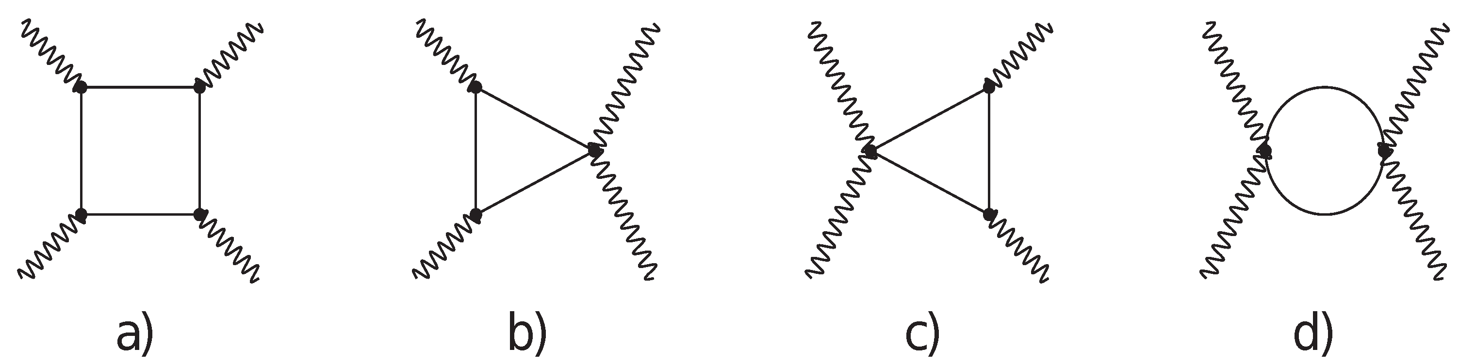
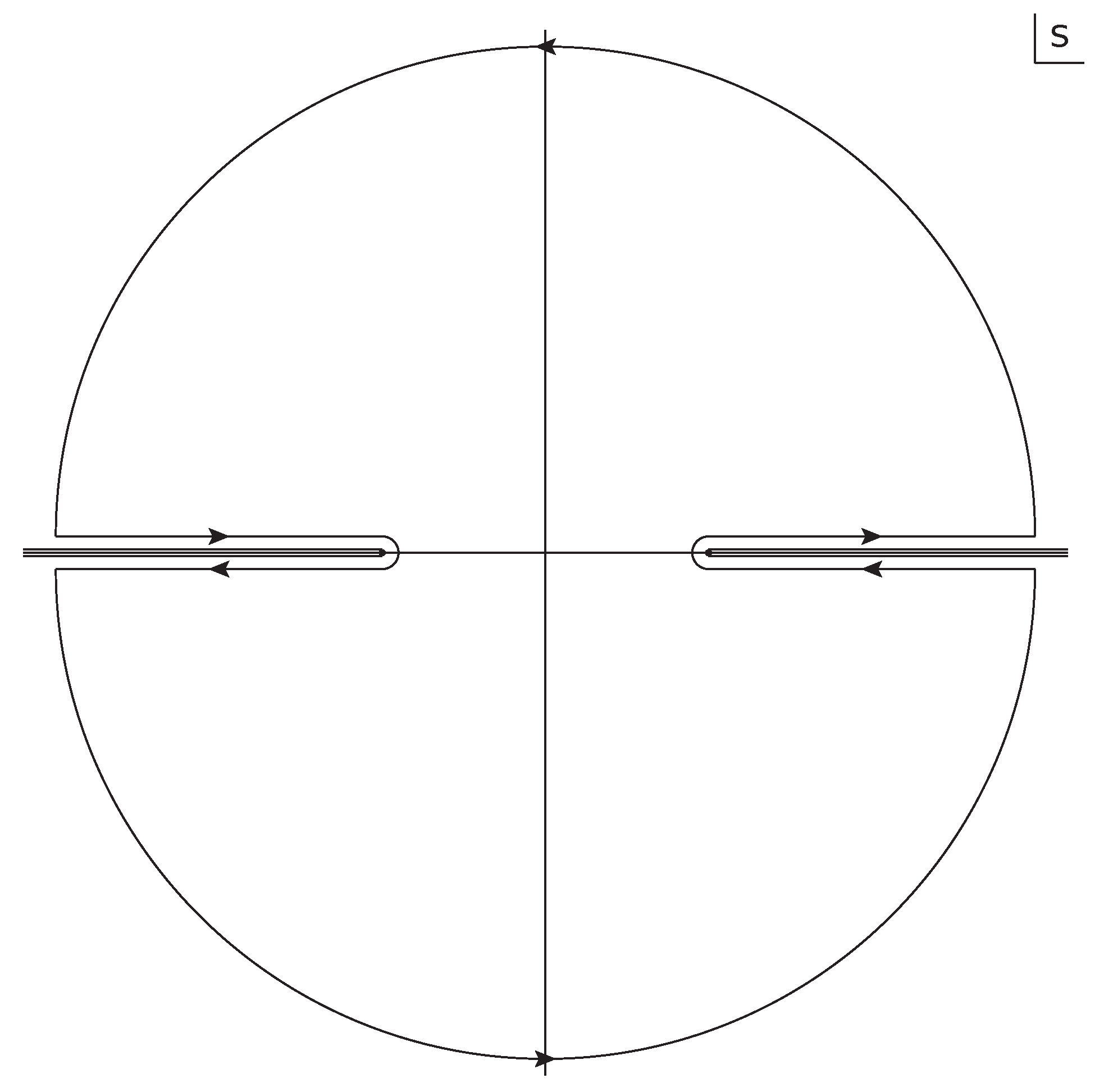
2. Calculation
3. Spin 0
4. Spin
5. Spin 1
6. Conclusions
Funding
Data Availability Statement
Acknowledgments
Conflicts of Interest
| 1 | |
| 2 | A similar approach was taken by Schwinger in [14]. |
References
- Euler, H. On the Scattering of Light by Light in Dirac’s Theory. Ph.D. Thesis, University of Leipzig, Leipzig, Germany, 1936. [Google Scholar]
- Dunne, G.V. The Euler-Heiseberg Effective Action: 75 Years On. Int. J. Mod. Phys. Conf. Ser. 2012, 14, 42–56. [Google Scholar] [CrossRef]
- Dittrich, W. Some Remarks on the Use of Effective Lagrangians in QED and QCD. Int. J. Mod. Phys. 2015, A30, 1530046. [Google Scholar] [CrossRef]
- Holstein, B.R. Evaluating the Effective Action. Found. Phys. 2000, 30, 413–437. [Google Scholar] [CrossRef]
- Heisenberg, W.; Euler, H. Consequences of Dirac’s Theory of Positrons. Z. Phys. 1936, 98, 714–732. [Google Scholar] [CrossRef]
- Weisskopf, V. The Electrodynamics of the Vacuum based on the Quantum Theory of the Electron. Kong. Dans. Vid. Selsk. Math-Phys. Med. 1936, 14N6, 1–39. [Google Scholar]
- Vanyashin, V.S.; Terent’ev, M.V. The Vacuum Polarization of a Charged Vector Field. Sov. Phys. JETP 1965, 21, 375. [Google Scholar]
- Aaboud, M. et al. [ATLAS Collaboration] Evidence for Light-by-Light Scattering in Heavy-Ion Collisions with the ATLAS Detector at the LHC. Nat. Phys. 2017, 13, 852–858. [Google Scholar] [CrossRef]
- Jegerlehner, F.; Nyffeler, A. The Muon g-2. Phys. Rept. 2009, 477, 1. [Google Scholar] [CrossRef]
- Preucil, F. Effective Interactions of the Euler-Heisenberg Type in Models of Quantum Field Theory. Master’s Thesis, Charles University, Staré Město, Czech, 2014. [Google Scholar]
- Preucil, F.; Horejsi, J. Effective Euler-Heisenberg Lagrangian in Models of QED. arXiv 2017, arXiv:1717.08106. [Google Scholar]
- Bjerrum-Bohr, N.E.J.; Donoghue, J.F.; Vanhove, P. On-shell Techniques and Universal Results in Quantum Gravity. J. High Energy Phys. 2014, 2014, 111. [Google Scholar] [CrossRef]
- Bjerrum-Bohr, N.E.J.; Damgaard, P.H.; Festuccia, G.; Planté, L. Pierre Vanhove General Relativity from Scattering Amplitudes. arXiv 2018, arXiv:1806.04920. [Google Scholar]
- Schwinger, J. Particles, Sources, and Fields; Addison-Wesley: Reading, MA, USA, 1973; Volume II. [Google Scholar]
- Pascalutsa, V.; Pauk, V.; Vanderhaeghen, M. Light-by-Light Scattering Sum Rules Constraining Meson Transition Form Factors. Phys. Rev. 2012, D85, 116001. [Google Scholar] [CrossRef]
- Pascalutsa, V. Causality Rules, a Light Treatise on Dispersion Relations and Sum Rules; IOP Publishing: Bristol, UK, 2018. [Google Scholar]
- Akhiezer, A.I.; Berestetskii, V.B. Quantum Electrodynamics; Wiley Interscience: New York, NY, USA, 1965. [Google Scholar]
- Pascalutsa, V.; Vanderhaeghen, M. Sum Rules for Light-by-Light Scattering. Phys. Rev. Lett. 2010, 105, 201603. [Google Scholar] [CrossRef] [PubMed]
- Gerasimov, S.B.; Moulin, J. Check of Sum Rules for Photon Interaction Cross-Sections in Quantum Electrodynamics and Mesodynamics. Yad. Fiz. 1976, 23, 142–153. [Google Scholar]
- Brodsky, S.J.; Schmidt, I. Classical Photoabsorption Sum Rules. Phys. Lett. 1995, B351, 344–348. [Google Scholar] [CrossRef]
- Gerasimov, S.B. A Sum Rule for Magnetic Moments and the Damping of the Nucleon Magnetic Moment in Nuclei. Yad. Fiz. 1965, 2, 598, Sov. J. Nucl. Phys.1966, 2, 430–433. [Google Scholar]
- Drell, S.D.; Hearn, A.C. Exact Sum Rule for Nucleon Magnetic Moments. Phys. Rev. Lett. 1966, 16, 908–911. [Google Scholar] [CrossRef]
- See, E.G.; Holstein, B.R. Graviton Physics. Am. J. Phys. 2006, 74, 1002–1011. [Google Scholar]
- Itzykson, C.; Zuber, J.-B. Quantum Field Theory; Dover: New York, NY, USA, 2005. [Google Scholar]
- Abarbanel, H.D.I.; Goldberger, M.L. Low-Energy Theorems, Dispersion Relations, and Superconvergence Sum Rules for Compton Scattering. Phys. Rev. 1968, 165, 1594–1609. [Google Scholar] [CrossRef]
- Bjerrum-Bohr, N.E.J.; Holstein, B.R.; Planté, L.; Vanhove, P. Graviton-Photon Scattering. Phys. Rev. 2015, D91, 064008. [Google Scholar] [CrossRef]
- Holstein, B.R. Analytical On-shell Calculation of Low-Energy Higher Order Scattering. J. Phys. 2017, G44, 01LT01. [Google Scholar] [CrossRef]
- Bjerrum-Bohr, N.E.J.; Donoghue, J.F.; Holstein, B.R. Quantum Gravitational Corrections to the Nonrelativistic Scattering Potential of Two Masses. Phys. Rev. 2003, D67, 084033. [Google Scholar] [CrossRef]
Disclaimer/Publisher’s Note: The statements, opinions and data contained in all publications are solely those of the individual author(s) and contributor(s) and not of MDPI and/or the editor(s). MDPI and/or the editor(s) disclaim responsibility for any injury to people or property resulting from any ideas, methods, instructions or products referred to in the content. |
© 2025 by the author. Licensee MDPI, Basel, Switzerland. This article is an open access article distributed under the terms and conditions of the Creative Commons Attribution (CC BY) license (https://creativecommons.org/licenses/by/4.0/).
Share and Cite
Holstein, B.R. On-Shell Calculation of Low-Energy Photon–Photon Scattering. Universe 2025, 11, 134. https://doi.org/10.3390/universe11050134
Holstein BR. On-Shell Calculation of Low-Energy Photon–Photon Scattering. Universe. 2025; 11(5):134. https://doi.org/10.3390/universe11050134
Chicago/Turabian StyleHolstein, Barry R. 2025. "On-Shell Calculation of Low-Energy Photon–Photon Scattering" Universe 11, no. 5: 134. https://doi.org/10.3390/universe11050134
APA StyleHolstein, B. R. (2025). On-Shell Calculation of Low-Energy Photon–Photon Scattering. Universe, 11(5), 134. https://doi.org/10.3390/universe11050134