Article

Searching for Gravitational-Wave Bursts from Cosmic String Cusps with the Parkes Pulsar Timing Array’s Third Data Release

1
Xinjiang Astronomical Observatories, Chinese Academy of Sciences, Urumqi 830011, China
2
University of Chinese Academy of Sciences, Beijing 100049, China
3
Institute of Optoelectronic Technology, Lishui University, Lishui 323000, China
4
Department of Physics, Nagoya University, Nagoya 464-8602, Japan
5
Instituto de Fisica Teorica UAM-CSIC, Universidad Autonoma de Madrid, 28049 Madrid, Spain
6
Xinjiang Key Laboratory of Radio Astrophysics, Urumqi 830011, China
7
School of Mathematical and Physical Sciences, Macquarie University, Sydney, NSW 2109, Australia
8
Research Center for Astronomical Computing, Zhejiang Laboratory, Hangzhou 311100, China
9
Institute for Astronomy, School of Physics, Zhejiang University, Hangzhou 310027, China
10
School of Physics and Astronomy, Monash University, Clayton, VIC 3800, Australia
11
OzGrav: The Australian Research Council Centre of Excellence for Gravitational Wave Discovery, Clayton, VIC 3800, Australia
12
Australia Telescope National Facility, CSIRO, Space and Astronomy, P.O. Box 76, Epping, NSW 1710, Australia
13
Centre for Astrophysics and Supercomputing, Swinburne University of Technology, P.O. Box 218, Hawthorn, VIC 3122, Australia
14
CSIRO Scientific Computing, Australian Technology Park, Locked Bag 9013, Alexandria, NSW 1435, Australia
15
Department of Physics, Faculty of Arts and Sciences, Beijing Normal University, Zhuhai 519087, China
16
Institute for Frontier in Astronomy and Astrophysics, Beijing Normal University, Beijing 102206, China
*
Authors to whom correspondence should be addressed.
Universe 2025, 11(3), 81; https://doi.org/10.3390/universe11030081
Submission received: 23 December 2024 / Revised: 22 February 2025 / Accepted: 25 February 2025 / Published: 1 March 2025
(This article belongs to the Special Issue Cosmological Models of the Universe)

Abstract

:
Pulsar timing arrays (PTAs) are designed to detect nanohertz-frequency gravitational waves (GWs). Since GWs are anticipated from cosmic strings, PTAs offer a viable approach to testing their existence. We present the results of the first Bayesian search for gravitational-wave bursts from cosmic string cusps (GWCSs) using the third PPTA data release for 30 ms pulsars. In this data collection, we find no evidence for GWCS signals. We compare a model with a GWCS signal to one with only noise, including a common spatially uncorrelated red noise (CURN), and find that our data are more consistent with the noise-only model. We then establish upper limits on the strain amplitude of GWCSs at the pulsar term, based on the analysis of 30 ms pulsars, after finding no compelling evidence. We find the addition of a CURN with different spectral indices into the noise model has a negligible impact on the upper limits. And the upper limit range of the amplitude of the pulsar-term GWCSs is concentrated between 10 12 and 10 11 . Finally, we set upper limits on the amplitude of GWCS events, parametrized by width and event epoch, for a single-pulsar PSR J1857 + 0943. Moreover, we derive the upper limit on the cosmic string tension as a function of burst width and compare it with previous results.

1. Introduction

Low-frequency GWs between 10 9 and 10 7 Hz can be detected with high sensitivity using a pulsar timing array (PTA), which consists of a group of millisecond pulsars with extremely stable rotational periods [1]. Owing to their stability, it is anticipated that timing residuals affected by a gravitational wave (GW) can be observed by closely monitoring the times of arrival (TOAs) of radio pulses from these millisecond pulsars [2]. Timing residuals are the discrepancies between the TOAs and the predictions of the pulsar timing model [3]. Factors other than GWs that can lead to timing residuals include clock faults, unmodeled variability in the solar wind, interstellar medium scattering, flaws in the solar system ephemeris (SSE), and offsets caused by the observational instrument [4]. Therefore, there will be a significant difficulty in detecting gravitational waves. The North American Nanohertz Observatory for Gravitational Waves (NANOGrav) [5], the European Pulsar Timing Array (EPTA) [6], the Parkes Pulsar Timing Array (PPTA) [7], and the Indian Pulsar Timing Array (InPTA) [8] are among the PTA collaborations that are currently in operation. These partnerships result in the International Pulsar Timing Array (IPTA) [9]. Furthermore, the first analyses from the Chinese Pulsar Timing Array (CPTA) [10] and the MeerTime Pulsar Timing Array (MPTA) [11] have been published recently.
PTAs are currently the most promising method for detecting nanohertz GWs, primarily generated by the inspiraling of supermassive black hole binaries (SMBHBs) [12]. The incoherent superposition of these binary systems produces a stochastic GW background. Recent studies by NANOGrav [13], PPTA [14], EPTA [15], and CPTA [10] have reported that the significance of a GW origin is between 2 σ and 4 σ . The observed correlations between pulsar timing residuals closely match the predicted Hellings–Downs pattern, a characteristic signature of such a background. This finding has significant implications for our understanding of supermassive black holes and the large-scale structure of the Universe.
Beyond the stochastic gravitational-wave background, PTA data can also be used to probe a variety of other astrophysical phenomena. For instance, continuous gravitational waves emitted by single supermassive black holes [16], known as continuous waves, can be detected or constrained using PTA observations. Additionally, PTAs are sensitive to gravitational wave memory [17,18], a permanent distortion of spacetime caused by extreme gravitational events like the merger of two black holes. Furthermore, PTAs can provide insights into the nature of dark matter [19]. By searching for characteristic signals from ultralight scalar-field dark matter, PTAs can constrain the properties of this elusive component of the Universe.
One particularly intriguing possibility is the detection of GWCSs, hypothetical defects in the fabric of spacetime that may have formed during the early Universe. Such bursts, if they exist, could be within the detectable frequency range of PTAs. Theoretical models suggest that a spontaneous symmetry-breaking phase transition in the early Universe [20] could have resulted in the formation of macroscopic, one-dimensional, stable, and highly energetic cosmic strings. Quantum field theory and condensed matter models predict these cosmic strings as topological defects, which play a role in various supersymmetric unified field theories, including D-brane models [21]. Initially, cosmic strings were proposed as a potential explanation for the formation of large-scale structure in the early Universe, with symmetry breaking occurring at the grand unification scale [22].
Due to the predicted emission of GWCSs, experiments like the PTAs offer a potential method to verify their existence. The most powerful GW bursts are generated at cusps, which are highly Lorentz-boosted singularities on string loops [20]. A cusp is a region in the loop that is highly Lorentz-boosted and produces a powerful beam of GWs. In general, the gravitational wave background is primarily the result of the overlap of multiple bursts. However, in specific regions of parameter space, a limited number of distinct GW bursts can contribute significantly to the overall background. A sufficiently large GW amplitude from such an event could render it detectable as a single burst. The Laser Interferometer Gravitational-Wave Observatory (LIGO) [23,24,25] has conducted searches for individual GWs from cosmic strings in the direction of fast radio burst sources. Leveraging the second data release from the PPTA project, Yonemaru et al. [21] performed the first search for GWCSs, employing a frequentist-based approach. In this paper, we will search and place limits on GWCSs based on the third PPTA data release (PPTA-DR3) using a Bayesian approach.
This paper is organized as follows. In Section 2, we provide a short description of PPTA-DR3. In Section 3, we examine the impact of GWCSs on TOAs from a PTA. We provide a concise overview of the Bayesian method and software employed in this search in Section 4. In Section 5, we demonstrate the implementation of the proposed algorithm on the PPTA data and discuss the resulting outcomes. Finally, the conclusion is presented in Section 6.

2. Data

This analysis is based on the PPTA-DR3 data and the noise analyses of individual pulsars. We will provide a concise summary of the most significant aspects of this dataset, with additional details available in the work of Zic et al. [26] and Reardon et al. [27].
The 64-meter Parkes “Murriyang” radio telescope was utilized to observe 32 pulsars, which are included in the release. Observations commenced in 2004, and the data were collected over the course of 18 years (MJD 53,040–59,640) consisting of approximately 48 h of observations made every 2–3 weeks. This release combines an updated version of the second PPTA data release (PPTA-DR2) with approximately three years of more recent data. The data were predominantly obtained using an ultra-wide-bandwidth receiver system that operates between 704 and 4032 MHz. One of the pulsars that was previously included in PPTA-DR2, PSR J1732 − 5049, was excluded due to the significant uncertainties in its TOAs, which resulted in periodic observations ceasing in 2011. Six additional binary pulsars (PSRs J0125 − 2327, J0614 − 3329, J0900 − 3144, J1741 + 1351, J1902 − 5105, and J1933 − 6211) and one solitary pulsar (PSR J0030 + 0451) are included in this release, in contrast to previous data releases. After the UWL receiver was commissioned, these pulsars were incorporated into PPTA observations, despite not having been previously included. In large part, the enhanced observation efficiency of the UWL receiver enabled the inclusion of these pulsars in the PPTA observations.
The dataset utilized for this analysis, which encompasses the pulsar ephemerides and TOAs, is detailed in Zic et al.’s work [26]. Commencing with the timing analyses of the preceding data releases [28,29], the initial timing models of each pulsar were fitted using TEMPO2 [3]. For the pulsars newly included in the PPTA following the release of PPTA-DR2, we adopt the initial timing models presented by Curyło et al. [30].
Despite the inclusion of observations from 32 pulsars in PPTA-DR3, we will analyze only 30 pulsars in this study. We excluded the globular cluster MSP PSR J1824 − 2452A because its steep-spectrum red noise is too intense for a common process to affect it. Although globular-cluster dynamics may also be involved, the disturbance is likely intrinsic to the pulsar [31]. This analysis, as well as the subsequent GWCS search, excludes PSR J1741 + 1351 because the dataset contains only 16 unique observations of this pulsar, which is insufficient for noise process simulation.

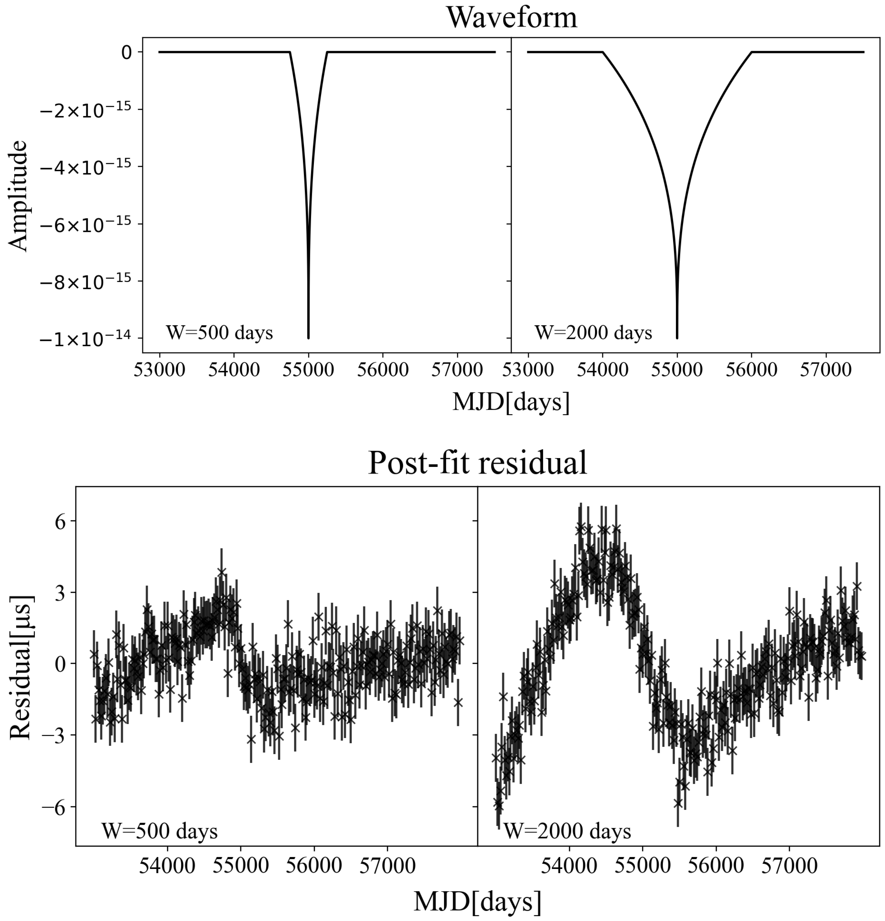
3. Signal of the GWCSs

We will examine the effect of GWCSs on TOA in pulsar timing data in this section and provide an extensive overview of the signal and noise models incorporated. A GW passing through a pulsar will induce a shift in the observed rotational frequency, which may result in either an increase or decrease in the frequency. When a GW passes through the Earth, the rotational frequencies observed for all pulsars in the PTA will be affected, leading to either an increase or decrease. The timing residuals induced by a GWCS will display distinct shapes depending on the epoch and duration of the burst, yet these shapes adhere to a deterministic pattern.
The timing residuals will be introduced as a result of the discrepancy between the observed rotational frequency and the pulsar’s timing model-fitted rotational frequency, regardless of the situation. Detweiler [32] provided the timing residuals induced by GWs:
r ( t ) = a = + , × F a ( Ω ^ , p ^ ) t Δ h a ( Ω ^ , t ) d t ,
where p ^ and Ω ^ are the directions of the pulsar and the GW propagation, respectively. F a ( Ω ^ , p ^ ) is the antenna pattern defined by Anholm et al. [33]:
F a ( Ω ^ , p ^ ) = 1 2 p ^ i p ^ j 1 + Ω ^ · p ^ e i j a ( Ω ^ ) .
The GW polarization tensors, denoted as e i j a ( a = + , × ) , are defined as follows:
e i j + ( Ω ^ ) = m i ^ m j ^ n i ^ n j ^
e i j × ( Ω ^ ) = m i ^ n j ^ + n i ^ m j ^ ,
where m ^ and n ^ are the polarization basis vectors. For ease of computation, we define
m ^ = s i n δ x ^ c o s δ y ^
n ^ = c o s α c o s δ x ^ c o s α s i n δ y ^ + s i n α z ^ ,
where x ^ , y ^ , and z ^ are unit vectors in the Cartesian coordinate system, and ( α , δ ) is the gravitational wave source position. Therefore, we can obtain
Ω ^ = s i n α c o s δ x ^ s i n α s i n δ y ^ c o s α z ^ ,
where Δ h a ( Ω ^ , t ) represents the metric perturbation difference between the Earth and the pulsar, as determined by the linearly polarized GWCSs. The time-domain waveform of a plus-polarized GWCS event is detailed by Yonemaru et al. [21]:
h + ( t ) = A fit t t 0 1 / 3 ( 1 2 W ) 1 / 3 ( t 0 1 2 W t < t 0 + 1 2 W ) 0 ( otherwise )
h × ( t ) = 0 ,
where A fit is the amplitude, t 0 is the epoch at which the burst peak arrives the Earth, and W is the duration of the burst. Strongly beamed in the direction of the cusp velocity is the GW burst, with cosmic string loops thought to generate cusps with high efficiency ( O ( 1 ) per oscillation period). The orientation is assumed to be random and depend on the string configuration [34]. It is important to mention that A fit carries dimensions of s 1 / 3 . The peak value at t = t 0 , which is dimensionless, is defined as follows:
A peak h + ( t 0 ) = 1 2 W 1 / 3 A fit .
By substituting Equation (8) into Equation (1), the analytic expressions for the pre-fit timing residual caused by the GWCSs are derived, using A fit , as follows:
r ( t ) = F + ( Ω ^ , p ^ ) × 0 ( t < t 0 W 2 ) A fit [ 3 4 W 2 4 / 3 | t t 0 | 4 / 3 W 2 1 / 3 t t 0 W 2 ] t 0 1 2 W t < t 0 + 1 2 W 1 4 ( 1 2 ) 1 / 3 A fit W 4 / 3 ( t t 0 + 1 2 W ) .
In the second line, the use of ∓ signifies that the − sign is to be placed before t 0 and the + after. The effect of GWCSs has been incorporated into the TEMPO2 timing model. This allows us to simulate residuals (or TOAs) of the GWCSs. The updated timing model parameters are ( A fit , t 0 , W , α , δ , ζ ) . Here, ζ is the principal polarization angle. This parametrization proves advantageous for the simulation of timing residuals induced by GWCSs. Introducing a second parametrization of the GW burst proves advantageous for the search procedure. The GW burst in this parametrization is represented by two orthogonal components, A 1 and A 2 , with A 1 = A fit cos(2 ζ ) and A 2 = A fit sin(2 ζ ). These components are associated with the two polarization modes of the GW, and this parametrization allows for the search of all possible GW polarizations. TEMPO2 software package allows the use of the following parameters in its parameter files: GWCS_A1, GWCS_A2, GWCS_POSITION, GWCS_EPOCH, and GWCS_WIDTH, which correspond to the cosmic string parameters A 1 , A 2 , sky position, burst epoch, and width, respectively.
Examples of the waveform and simulated timing residuals are shown in Figure 1. The PTASIMULATE software package was used to simulate cosmic string burst events as described above. We assume that the position and polarization angle of the gravitational wave source are ( α = 57 . 3 , δ = 57 . 3 ) and ζ = 30 , respectively. Timing residuals are produced by infusing a GWCS signal with an amplitude of A peak = 10 14 at the center of the observation (MJD 55,000) and 1 μ s of Gaussian white noise using Equation (11). The burst widths are set to 500 days (panel on the left side) and 2000 days (panel on the right side), corresponding to A fit = 1.59 × 10 15 and 1.0 × 10 15 , respectively.
Because of the crucial role of detecting a common spatially uncorrelated red noise process (CURN) identified by NANOGrav, PPTA, EPTA, and CPTA, a CURN with a specified spectral index is thus included in our model. A power-law can be used to model the CURN, with its power spectrum governed by two hyperparameters, ( A , γ ) [35]:
P ( f ) = A 2 f yr 1 γ ,
Here, f denotes the frequency of the spectral component, A represents the characteristic amplitude of the red noise process at a frequency of yr 1 , and γ is the spectral index associated with the characteristic amplitude. The spectral index of a stochastic gravitational wave background, arising from an ensemble of supermassive black hole binaries, is expected to be 4.33. However, the spectral index of the CURN was found to have a maximum a posteriori value of 5.5 [36]. In this paper, we present two sets of results for the CURN that utilize both of these fixed spectral indices ( γ CURN = 4.33 and 5.5 ).

4. Methods

We used the Markov Chain Monte Carlo (MCMC) approach for the search of GWCSs. In this section, we will provide a concise summary of the techniques. The methods employed in this search are detailed in the works of Sun et al. [37] and Aggarwal et al. [38] to search for gravitational wave memory and continuous gravitational wave signals. The TOA residuals for an individual pulsar can be represented as a combination of multiple stochastic deterministic and stochastic processes:
δ t = δ t cs + M ϵ + F a + F gw a gw + n .
where δ t represents the residual time series for the pulsar. The term δ t cs denotes the residuals induced by GWCSs. M is the design matrix representing the linearized timing model, which is responsible for accounting for the uncertainty in the residuals resulting from an imperfect timing model fit ϵ . The design matrix F corresponds to the pulsar’s intrinsic Gaussian red noise process, modeled as a Fourier series with coefficients represented by a. Likewise, F gw and a gw are the design matrix and Fourier coefficients for the CURN, respectively. Lastly, the elements of vector n represent uncertainty in the observed TOAs, which follow a Gaussian white noise distribution.
Based on the estimations of the Gaussian process parameters, GWCS signal, and timing model parameters, it is possible to generate residuals n:
n = δ t δ t cs M ϵ F a F gw a gw .
As the terms on the right-hand side are approximations, this constitutes merely an estimation of white noise. Nevertheless, assuming the white noise follows a Gaussian distribution, the likelihood of observing this specific sequence of white noise residuals can be expressed as
p ( n ) = e x p ( 1 2 n T N 1 n ) 2 π d e t N .
Above, N is a covariance matrix that represents the white noise uncertainties in each observed TOA, and n T is the transpose of n.
After the removal of deterministic effects, the remaining pulsar timing residuals have the same likelihood of following a Gaussian white noise distribution as the detection of a GWCS signal. This means that
p ( δ t ϵ , a , a gw , A fit , t 0 , W , Ω ^ , p ^ , ζ ) = e x p ( 1 2 n T N 1 n ) 2 π d e t N .
The parameter space dimensionality can be reduced through the analytical marginalization of the likelihood in Equation (16) with respect to the parameters that describe the Gaussian processes [39,40,41]. The final marginalized likelihood obtained is
p ( δ t A fit , W , t 0 , Ω ^ , p ^ , ζ ) = e x p ( 1 2 q T C 1 q ) 2 π d e t C ,
where the following definitions are provided:
q = δ t δ t cs ,
C = N + T D T T ,
T = M F ,
D = 0 0 ϕ ,
where is a diagonal matrix of infinities, which effectively provides unconstrained priors on the timing model parameters. ϕ is a covariance matrix that represents the individual red noise and the CURN Fourier coefficients. As a result of employing a CURN, the ϕ matrices are diagonal, with each diagonal element representing the red noise power at the corresponding frequency bin, as specified in Equation (12). C 1 is efficiently computed using the Woodbury matrix identity [42]. In this identity, the matrix D is present solely as an inverse. As a result, the diagonal matrix containing infinities is effectively replaced by a matrix of zeros during the likelihood calculation.
We favored ignorance priors for our model parameters and implemented uniform or log-uniform priors for all. We employed the same priors for noise parameters as those used by Reardon et al. [27] and Reardon et al. [14]. Table 1 provides the prior distributions of model parameters in the Bayesian Search for Global GWCSs using the full PTA that we are interested in. The Bayes factor, denoted as B gw , was employed as the detection statistic to compare the GW model with a noise-only model. Bayes factor was computed using the Savage–Dickey approximation, as described by Dickey [43]:
B gw = ε gw ε noise lim A fit 0 p ( A fit ) p ( A fit | δ t ) .
The evidence ratio ( ε gw / ε noise ) for the GW and noise-only models can be approximated as the ratio of the prior to posterior probability as the GW amplitude approaches zero. This computation is significantly more computationally efficient than a complete evidence integral, as it employs posterior samples that are located near the low-amplitude prior boundary.
This likelihood calculation and these signal models were implemented in the ENTERPRISE [44] and ENTERPRISE_EXTENSIONS [45]. The PTMCMCSAMPLER [46] package implements the MCMC sampler to extract samples from the posterior distributions.

5. Results

5.1. Earth-Term GWCS Search

By applying MCMC sampling, we initiated a Bayesian search for GWCSs in the Earth term, contrasting two models: (1) a noise-only model and (2) a model that includes both noise and the GWCS signal. The noise-only model included white noise, achromatic red noise (Red), dispersion measure (DM), high fluctuation frequency (HFF), chromatic (Chr), low-frequency band noise (BN), and a CURN process [14]. The signal model incorporated identical noise processes together with GWCS signals. We employed the product-space sampling technique [47] to sample both models simultaneously. This allowed us to determine the posterior probability for the GWCS signal and compute the Bayes factor of B gw = 0.7 for the GWCS signal model. Compared to the noise-only model, this Bayes factor is too small to be considered detected. Figure 2 illustrates the posterior probability distributions for the GWCS signal as well as the global spatially uncorrelated red noise process.
By analyzing the posterior distribution, we can pinpoint geographically significant areas of high activity near MJDs 54,000. The feature near MJD 54,000 is situated approximately in the beginning of our observations, during a period when there were significant gaps in data for multiple pulsars. At the beginning of our dataset, there was a small number of pulsars being observed, and the observations exhibited less regularity. Data sparsity complicates the task of constraining any signal in this time. A heightened degeneracy is observed for events occurring earlier in the dataset when a quadratic pulsar timing model is applied to the pulsar’s rotational frequency and its derivative. This implies that the signal model can exhibit consistency with a GWCS event of significant magnitude, which is appropriately eliminated by the marginalization of the timing model.

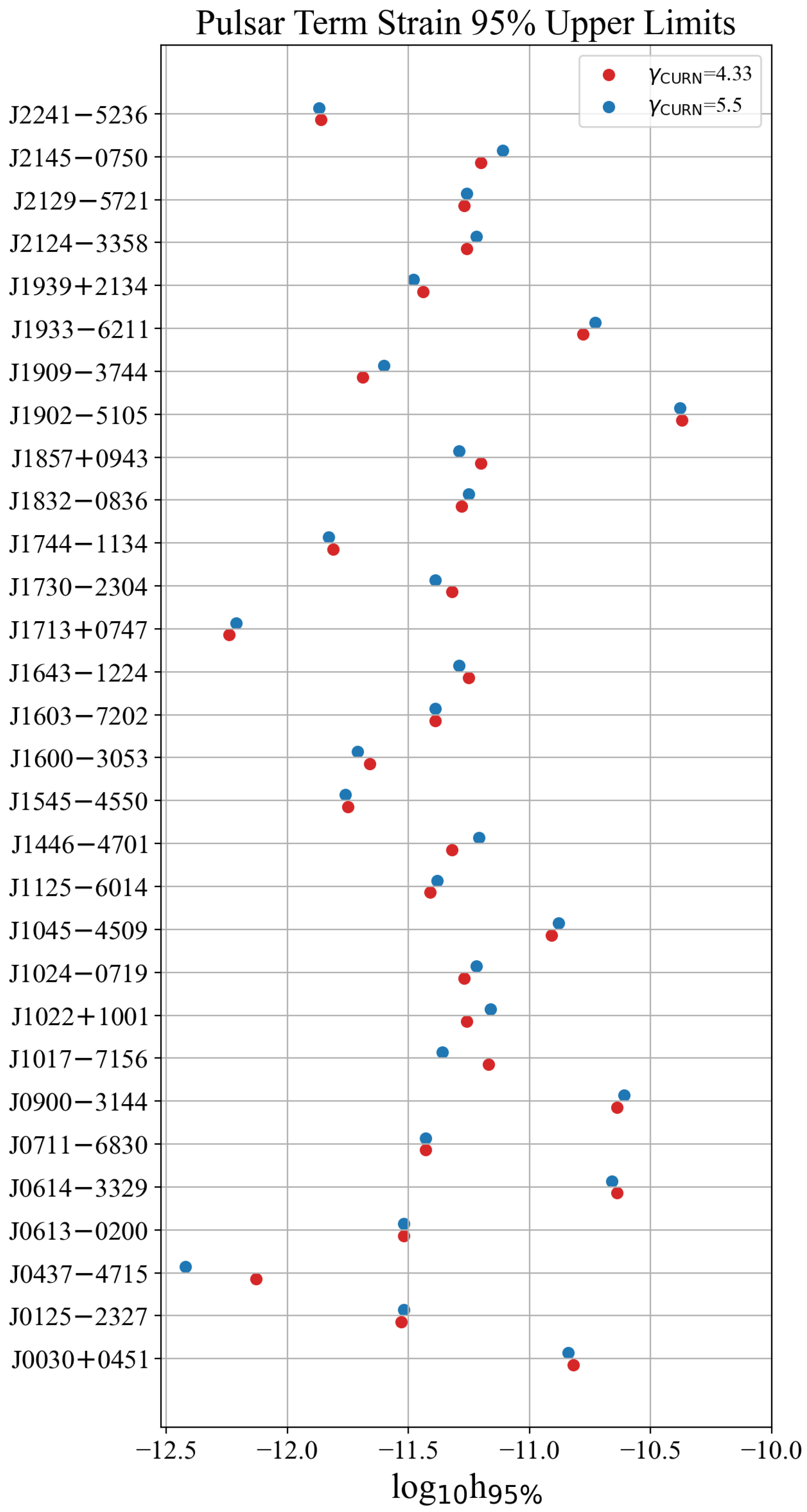
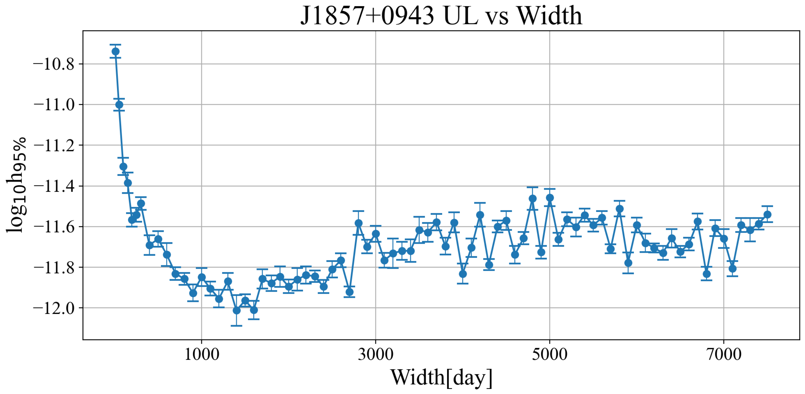
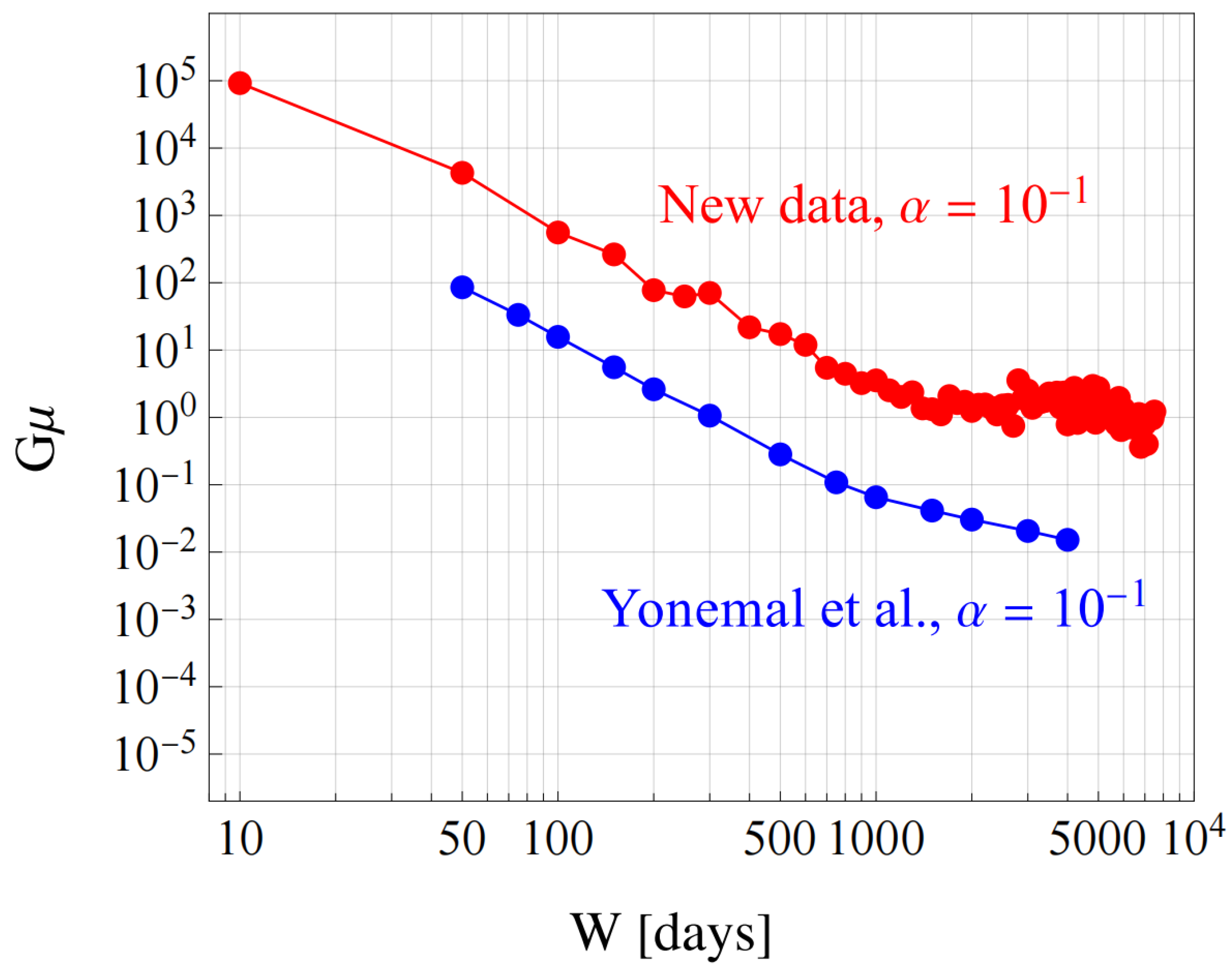
5.2. Pulsar-Term Upper Limits

It is almost impossible to make a confident detection with a single pulsar term search of GWCSs, but we could still use non-detection in the pulsar term search to set upper limits. We report upper limits on the amplitude of the GWCS strain. The pulsar-term upper limits on GWCSs are illustrated in Figure 3, which employs both fixed spectral indices ( γ CURN = 4.33 and 5.5 ). As the pulsar-term upper limits are calculated individually for each pulsar, any information about the signal’s sky location is effectively lost. This means that it becomes challenging to distinguish between a weak GWCS event and one that originates from a sky location where the antenna pattern is weak relative to the position of the pulsar.
The upper limit A fit is determined by setting the width at W = 100 days, and then we calculate the upper limit h for the pulsar term using Equation (10). It is evident that the pulsar-term upper limits are not significantly influenced by the selection of spectral index for the majority of pulsars.
The constraints on h can be expressed as a mathematical function that depends on the epoch, width, and sky position. Only the width has a physical significance, which is equivalent to the loop size of the cosmic string. In Figure 4, we obtained the upper limit h as a function of the width for PSR J1857 + 0943. The early- and late-time bursts lack credibility due to insufficient data available prior to or following the occurrence of these bursts, which hinders the ability to accurately determine their amplitude. As the width increases, the constraint on h becomes more stringent since the timing residuals caused by the GWCSs increase as the event duration increases. In Figure 4, the upper limit h is a function of the width. As width increases, the strain amplitude h decreases, then increases, and finally plateaus. The limitation is strongest when the width is about 1200 days and the upper limit is about 10 12 .
A term specific to each pulsar is introduced to impose a constraint on the upper time analysis for individual pulsars within the array. The upper bound h is a function of the burst epoch t 0 by fixing W = 100 days for PSR 1857 + 0943 in Figure 5. When epoch t 0 is the median value, the upper limit of the amplitude stabilizes, and the constraint on h is the weakest at the beginning and end. When epoch t 0 is about 59,000, the GWCS strain amplitude upper limit is possibly the strongest because of a new ultra-wideband receiver.
Here, we translate the upper bound on the peak amplitude shown in Figure 4 into a constraint on the cosmic string tension. The upper bounds on the time-domain amplitude with different widths shown in Figure 4 can be translated into the Fourier strain amplitude h ˜ lim . The expected number of gravitational wave bursts from cosmic string cusps reaching Earth today with amplitudes exceeding h ˜ lim is denoted as N GWCS . Given the absence of detected cosmic string GW bursts with amplitudes above h ˜ lim , a random Poisson process analysis at the 95% confidence level excludes scenarios where N GWCS > 2.996 . Using this constraint, we establish an upper limit on the cosmic string tension. Details of the translation can be found in [21].
Figure 6 presents the constraint on the cosmic string tension as a function of burst width W, derived from the single-pulsar dataset of PSR 1857 + 0943, alongside the results from [21]. The α in Figure 6 represents the size of the primordial string loop, and here, we compare the cosmic string tension limit specifically for α = 0.1. As shown in Figure 6, the upper bound becomes more constraining for larger W due to two factors. First, as shown in Figure 4, the upper bound improves for larger W. Second, larger loops produce stronger GW amplitudes but have lower number densities. While the former enhances detectability, the latter reduces it. Considering both effects, we find that the former effect dominates, and that larger loops, equivalently larger W, are easier to detect, leading to tighter constraints.
However, the upper limit from [21] is more than an order of magnitude tighter than our results. This discrepancy arises because we only used the dataset of a single pulsar (pulsar term), whereas Yonemaru et al. [21] utilized the full PPTA dataset (Earth term). Additionally, MCMC sampling is very computationally intensive and time-consuming. In future work, we plan to extend our analysis to include the Earth-term search.
So far, only Yonemaru et al. [21] and this work have studied individual GW bursts from cosmic string cusps using PTA. In addition, cosmic string parameters can also be constrained by the cosmic microwave background (CMB) [48] and the stochastic GW background. While the stochastic background provides a stronger constraint on string parameters, we emphasize that GW burst searches offer independent constraints. The future SKA telescope will observe a large number of millisecond pulsars with high timing precision. With the improved sensitivity of SKA, the prospects for detecting single GW bursts will be significantly enhanced. A stringent constraint on the cosmic string tension from SKA would be highly valuable for testing various models of cosmic superstrings, such as the KKLMMT model [49].

6. Conclusions

In this paper, we present the first Bayesian search for the GWCSs using PPTA-DR3; there is no significant evidence of GWCSs. Therefore, we place upper limits on the strain amplitude of pulsar-term GWCSs for the 30 ms pulsars. We find that incorporating a CURN with various spectral indices into the noise model has a negligible impact on the upper limits. And the upper limit range of the amplitude of the pulsar-term GWCSs is concentrated between 10 12 and 10 11 . By analyzing an individual pulsar PSR J1857 + 0943, we place upper limits on the amplitude of GWCS events as a function of width and event epoch. We obtain the upper limit on the cosmic string tension as a function of burst width and will present the results of all-sky Earth-term upper limits in future work. With its improved sensitivity, SKA will place significantly tighter constraints on cosmic string parameters, making it a valuable tool for testing cosmic string models. Moreover, such constraints will provide an independent probe for investigating the clustering of cosmic string loops in our Galaxy, which cannot be tested through CMB analysis or stochastic GW background.

Author Contributions

Software, Y.X. and Y.W.; investigation, J.W., S.K., Y.F., S.M., C.J.R., S.W. and D.Z.; data curation, Y.X. and Y.W.; writing—original draft preparation, Y.X.; writing—review and editing, J.W., W.Y. and A.K.; visualization, Y.X., S.K. and J.Z.; funding acquisition, J.W., W.Y., V.D.M. and X.Z. All authors have read and agreed to the published version of the manuscript.

Funding

This research was funded by the Major Science and Technology Program of Xinjiang Uygur Autonomous Region (No. 2022A03013-4), the Zhejiang Provincial Natural Science Foundation of China (No. LY23A030001), the Natural Science Foundation of Xinjiiang Uygur Autonomous Region (No. 2022D01D85), National Natural Science Foundation of China (No. 12041304); W.M.Y. is supported by the National Natural Science Foundation of China (NSFC) project (No. 12273100, 12041303), the West Light Foundation of Chinese Academy of Sciences (No. WLFC 2021-XBQNXZ-027), the National Key Program for Science and Technology Research and Development and the National SKA Program of China (No. 2022YFC2205201, 2020SKA0120200); V.D.M. is supported by the Australian Research Council (ARC) Centre of Excellence CE170100004 and CE230100016, and receives support from the Australian Government Research Training Program; X.J.Z. is supported by the National Natural Science Foundation of China (Grant No. 12203004) and by the Fundamental Research Funds for the Central Universities.

Data Availability Statement

Observational data used in this paper are quoted from the cited works. Additional data generated from computations can be made available upon reasonable request.

Acknowledgments

The Murriyang Parkes 64 m radio telescope, part of the Australia Telescope National Facility, is funded by the Australian Government and operated as a National Facility under CSIRO’s management. We acknowledge the Wiradjuri People as the Traditional Custodians of the land upon which the Observatory is located. We also pay respect to the Wurundjeri People of the Kulin Nation and the Wallumedegal People of the Darug Nation, the Traditional Owners of the land where this research was primarily carried out. Our heartfelt thanks go to the Parkes Observatory staff for their steadfast support over nearly twenty years. We are also thankful for the access provided by the CSIRO Information Management and Technology High-Performance Computing group to the Petrichor cluster and their technical assistance.

Conflicts of Interest

The authors declare no conflicts of interest.

Abbreviations

The following abbreviations are used in this manuscript:
PTAPulsar timing array
GWsGravitational waves
GWCSsGravitational-wave bursts from cosmic string cusps
CURNCommon spatially uncorrelated red noise

References

  1. Foster, R.S.; Backer, D.S. Constructing a Pulsar Timing Array. Astrophys. J. 1990, 361, 300. [Google Scholar] [CrossRef]
  2. Hellings, R.; Downs, G. Upper limits on the isotropic gravitational radiation background from pulsar timing analysis. Astrophys. J. 1983, 265, L39–L42. [Google Scholar] [CrossRef]
  3. Edwards, R.T.; Hobbs, G.; Manchester, R. TEMPO2, a new pulsar timing package–II. The timing model and precision estimates. Mon. Not. R. Astron. Soc. 2006, 372, 1549–1574. [Google Scholar] [CrossRef]
  4. Tiburzi, C.; Hobbs, G.; Kerr, M.; Coles, W.; Dai, S.; Manchester, R.; Possenti, A.; Shannon, R.; You, X. A study of spatial correlations in pulsar timing array data. Mon. Not. R. Astron. Soc. 2016, 455, 4339–4350. [Google Scholar] [CrossRef]
  5. Jenet, F.; Finn, L.; Lazio, J.; Lommen, A.; McLaughlin, M.; Stairs, I.; Stinebring, D.; Verbiest, J.; Archibald, A.; Arzoumanian, Z.; et al. The north american nanohertz observatory for gravitational waves. arXiv 2009, arXiv:0909.1058. [Google Scholar]
  6. Kramer, M.; Champion, D.J. The European pulsar timing array and the large European array for pulsars. Class. Quantum Gravity 2013, 30, 224009. [Google Scholar] [CrossRef]
  7. Manchester, R. The international pulsar timing array. Class. Quantum Gravity 2013, 30, 224010. [Google Scholar] [CrossRef]
  8. Nobleson, K.; Agarwal, N.; Girgaonkar, R.; Pandian, A.; Joshi, B.C.; Krishnakumar, M.; Susobhanan, A.; Desai, S.; Prabu, T.; Bathula, A.; et al. Low-frequency wideband timing of InPTA pulsars observed with the uGMRT. Mon. Not. R. Astron. Soc. 2022, 512, 1234–1243. [Google Scholar] [CrossRef]
  9. Verbiest, J.; Lentati, L.; Hobbs, G.; van Haasteren, R.; Demorest, P.B.; Janssen, G.; Wang, J.B.; Desvignes, G.; Caballero, R.; Keith, M.; et al. The international pulsar timing array: First data release. Mon. Not. R. Astron. Soc. 2016, 458, 1267–1288. [Google Scholar] [CrossRef]
  10. Xu, H.; Chen, S.; Guo, Y.; Jiang, J.; Wang, B.; Xu, J.; Xue, Z.; Caballero, R.N.; Yuan, J.; Xu, Y.; et al. Searching for the nano-Hertz stochastic gravitational wave background with the Chinese Pulsar Timing Array Data Release I. Res. Astron. Astrophys. 2023, 23, 075024. [Google Scholar] [CrossRef]
  11. Miles, M.T.; Shannon, R.M.; Bailes, M.; Reardon, D.J.; Keith, M.J.; Cameron, A.D.; Parthasarathy, A.; Shamohammadi, M.; Spiewak, R.; van Straten, W.; et al. The MeerKAT pulsar timing array: First data release. Mon. Not. R. Astron. Soc. 2023, 519, 3976–3991. [Google Scholar] [CrossRef]
  12. Burke-Spolaor, S.; Taylor, S.R.; Charisi, M.; Dolch, T.; Hazboun, J.S.; Holgado, A.M.; Kelley, L.Z.; Lazio, T.J.W.; Madison, D.R.; McMann, N.; et al. The astrophysics of nanohertz gravitational waves. Astron. Astrophys. Rev. 2019, 27, 1–78. [Google Scholar] [CrossRef]
  13. Agazie, G.; Anumarlapudi, A.; Archibald, A.M.; Arzoumanian, Z.; Baker, P.T.; Bécsy, B.; Blecha, L.; Brazier, A.; Brook, P.R.; Burke-Spolaor, S.; et al. The NANOGrav 15 yr data set: Evidence for a gravitational-wave background. Astrophys. J. Lett. 2023, 951, L8. [Google Scholar] [CrossRef]
  14. Reardon, D.J.; Zic, A.; Shannon, R.M.; Hobbs, G.B.; Bailes, M.; Di Marco, V.; Kapur, A.; Rogers, A.F.; Thrane, E.; Askew, J.; et al. Search for an isotropic gravitational-wave background with the Parkes Pulsar Timing Array. Astrophys. J. Lett. 2023, 951, L6. [Google Scholar] [CrossRef]
  15. Antoniadis, J.; Arumugam, P.; Arumugam, S.; Babak, S.; Bagchi, M.; Nielsen, A.S.B.; Bassa, C.; Bathula, A.; Berthereau, A.; Bonetti, M.; et al. The second data release from the European Pulsar Timing Array-III. Search for gravitational wave signals. Astron. Astrophys. 2023, 678, A50. [Google Scholar]
  16. Zhu, X.J.; Hobbs, G.; Wen, L.; Coles, W.A.; Wang, J.B.; Shannon, R.M.; Manchester, R.N.; Bailes, M.; Bhat, N.; Burke-Spolaor, S.; et al. An all-sky search for continuous gravitational waves in the Parkes Pulsar Timing Array data set. Mon. Not. R. Astron. Soc. 2014, 444, 3709–3720. [Google Scholar] [CrossRef]
  17. Wang, J.; Hobbs, G.; Coles, W.; Shannon, R.M.; Zhu, X.; Madison, D.; Kerr, M.; Ravi, V.; Keith, M.J.; Manchester, R.N.; et al. Searching for gravitational wave memory bursts with the Parkes Pulsar Timing Array. Mon. Not. R. Astron. Soc. 2015, 446, 1657–1671. [Google Scholar] [CrossRef]
  18. Agazie, G.; Arzoumanian, Z.; Baker, P.T.; Bécsy, B.; Blecha, L.; Blumer, H.; Brazier, A.; Brook, P.R.; Burke-Spolaor, S.; Burnette, R.; et al. The NANOGrav 12.5 yr Data Set: Search for Gravitational Wave Memory. Astrophys. J. 2024, 963, 61. [Google Scholar] [CrossRef]
  19. Porayko, N.K.; Zhu, X.; Levin, Y.; Hui, L.; Hobbs, G.; Grudskaya, A.; Postnov, K.; Bailes, M.; Bhat, N.R.; Coles, W.; et al. Parkes Pulsar Timing Array constraints on ultralight scalar-field dark matter. Phys. Rev. D 2018, 98, 102002. [Google Scholar] [CrossRef]
  20. Damour, T.; Vilenkin, A. Gravitational wave bursts from cosmic strings. Phys. Rev. Lett. 2000, 85, 3761. [Google Scholar] [CrossRef]
  21. Yonemaru, N.; Kuroyanagi, S.; Hobbs, G.; Takahashi, K.; Zhu, X.; Coles, W.; Dai, S.; Howard, E.; Manchester, R.; Reardon, D.; et al. Searching for gravitational-wave bursts from cosmic string cusps with the Parkes Pulsar Timing Array. Mon. Not. R. Astron. Soc. 2021, 501, 701–712. [Google Scholar] [CrossRef]
  22. Dvali, G.; Vilenkin, A. Formation and evolution of cosmic D strings. J. Cosmol. Astropart. Phys. 2004, 2004, 010. [Google Scholar] [CrossRef]
  23. Abbott, B.P.; Abbott, R.; Adhikari, R.; Ajith, P.; Allen, B.; Allen, G.; Amin, R.; Anderson, S.; Anderson, W.; Arain, M.; et al. First LIGO search for gravitational wave bursts from cosmic (super) strings. Phys. Rev. D—Part. Fields Gravit. Cosmol. 2009, 80, 062002. [Google Scholar] [CrossRef]
  24. Abbott, B.P.; Abbott, R.; Abbott, T.; Abernathy, M.; Acernese, F.; Ackley, K.; Adams, C.; Adams, T.; Addesso, P.; Adhikari, R.; et al. Search for transient gravitational waves in coincidence with short-duration radio transients during 2007–2013. Phys. Rev. D 2016, 93, 122008. [Google Scholar]
  25. Abbott, B.P.; Abbott, R.; Abbott, T.D.; Acernese, F.; Ackley, K.; Adams, C.; Adams, T.; Addesso, P.; Adhikari, R.X.; Adya, V.B.; et al. Constraints on cosmic strings using data from the first Advanced LIGO observing run. Phys. Rev. D 2018, 97, 102002. [Google Scholar] [CrossRef]
  26. Zic, A.; Reardon, D.J.; Kapur, A.; Hobbs, G.; Mandow, R.; Curyło, M.; Shannon, R.M.; Askew, J.; Bailes, M.; Bhat, N.R.; et al. The parkes pulsar timing array third data release. Publ. Astron. Soc. Aust. 2023, 40, e049. [Google Scholar] [CrossRef]
  27. Reardon, D.J.; Zic, A.; Shannon, R.M.; Di Marco, V.; Hobbs, G.B.; Kapur, A.; Lower, M.E.; Mandow, R.; Middleton, H.; Miles, M.T.; et al. The gravitational-wave background null hypothesis: Characterizing noise in millisecond pulsar arrival times with the Parkes Pulsar Timing Array. Astrophys. J. Lett. 2023, 951, L7. [Google Scholar] [CrossRef]
  28. Reardon, D.; Hobbs, G.; Coles, W.; Levin, Y.; Keith, M.; Bailes, M.; Bhat, N.; Burke-Spolaor, S.; Dai, S.; Kerr, M.; et al. Timing analysis for 20 millisecond pulsars in the Parkes Pulsar Timing Array. Mon. Not. R. Astron. Soc. 2016, 455, 1751–1769. [Google Scholar] [CrossRef]
  29. Reardon, D.J.; Shannon, R.M.; Cameron, A.D.; Goncharov, B.; Hobbs, G.; Middleton, H.; Shamohammadi, M.; Thyagarajan, N.; Bailes, M.; Bhat, N.; et al. The Parkes pulsar timing array second data release: Timing analysis. Mon. Not. R. Astron. Soc. 2021, 507, 2137–2153. [Google Scholar] [CrossRef]
  30. Curyło, M.; Pennucci, T.T.; Bailes, M.; Bhat, N.R.; Cameron, A.D.; Dai, S.; Hobbs, G.; Kapur, A.; Manchester, R.N.; Mandow, R.; et al. Wide-band timing of the Parkes Pulsar Timing Array UWL data. Astrophys. J. 2023, 944, 128. [Google Scholar] [CrossRef]
  31. Shannon, R.M.; Cordes, J.M. Assessing the role of spin noise in the precision timing of millisecond pulsars. Astrophys. J. 2010, 725, 1607. [Google Scholar] [CrossRef]
  32. Detweiler, S. Pulsar timing measurements and the search for gravitational waves. Astrophys. J. 1979, 234, 1100–1104. [Google Scholar] [CrossRef]
  33. Anholm, M.; Ballmer, S.; Creighton, J.D.; Price, L.R.; Siemens, X. Optimal strategies for gravitational wave stochastic background searches in pulsar timing data. Phys. Rev. D-Part. Fields Gravit. Cosmol. 2009, 79, 084030. [Google Scholar] [CrossRef]
  34. Blanco-Pillado, J.; Olum, K.D. Form of cosmic string cusps. Phys. Rev. D 1999, 59, 063508. [Google Scholar] [CrossRef]
  35. Phinney, E. A practical theorem on gravitational wave backgrounds. arXiv 2001, arXiv:astro-ph/0108028. [Google Scholar]
  36. Arzoumanian, Z.; Baker, P.T.; Blumer, H.; Bécsy, B.; Brazier, A.; Brook, P.R.; Burke-Spolaor, S.; Chatterjee, S.; Chen, S.; Cordes, J.M.; et al. The NANOGrav 12.5 yr data set: Search for an isotropic stochastic gravitational-wave background. Astrophys. J. Lett. 2020, 905, L34. [Google Scholar] [CrossRef]
  37. Sun, J.; Baker, P.T.; Johnson, A.D.; Madison, D.R.; Siemens, X. Implementation of an efficient bayesian search for gravitational-wave bursts with memory in pulsar timing array data. Astrophys. J. 2023, 951, 121. [Google Scholar] [CrossRef]
  38. Aggarwal, K.; Arzoumanian, Z.; Baker, P.; Brazier, A.; Brook, P.; Burke-Spolaor, S.; Chatterjee, S.; Cordes, J.; Cornish, N.; Crawford, F.; et al. The NANOGrav 11 yr data set: Limits on gravitational wave memory. Astrophys. J. 2020, 889, 38. [Google Scholar] [CrossRef]
  39. Lentati, L.; Alexander, P.; Hobson, M.P.; Taylor, S.; Gair, J.; Balan, S.T.; van Haasteren, R. Hyper-efficient model-independent Bayesian method for the analysis of pulsar timing data. Phys. Rev. D-Part. Fields Gravit. Cosmol. 2013, 87, 104021. [Google Scholar] [CrossRef]
  40. van Haasteren, R.; Vallisneri, M. New advances in the Gaussian-process approach to pulsar-timing data analysis. Phys. Rev. D 2014, 90, 104012. [Google Scholar] [CrossRef]
  41. van Haasteren, R.; Vallisneri, M. Low-rank approximations for large stationary covariance matrices, as used in the Bayesian and generalized-least-squares analysis of pulsar-timing data. Mon. Not. R. Astron. Soc. 2015, 446, 1170–1174. [Google Scholar] [CrossRef]
  42. Woodbury, M.A. Inverting Modified Matrices; Statistical Research Group, Memorandum Report No. 42; Princeton University: Princeton, NJ, USA, 1950. [Google Scholar]
  43. Dickey, J.M. The weighted likelihood ratio, linear hypotheses on normal location parameters. Ann. Math. Stat. 1971, 42, 204–223. [Google Scholar] [CrossRef]
  44. Ellis, J.A.; Vallisneri, M.; Taylor, S.R.; Baker, P.T. ENTERPRISE: Enhanced Numerical Toolbox Enabling a Robust PulsaR Inference SuitE, version 3.0.0; Zenodo: Geneva, Switzerland, 2020. [Google Scholar] [CrossRef]
  45. Taylor, S.R.; Baker, P.T.; Hazboun, J.S.; Simon, J.; Vigeland, S.J. enterprise_extensions; versio 2.4.3; GitHub, Inc.: San Francisc, CA, USA, 2021; Available online: https://github.com/nanograv/enterprise_extensions (accessed on 22 December 2024).
  46. Ellis, J.; Van Haasteren, R. Jellis18/Ptmcmcsampler: Official Release, version 1.0.0; Zenodo: Geneva, Switzerland, 2017; Available online: https://ui.adsabs.harvard.edu/abs/2017zndo...1037579E (accessed on 22 December 2024).
  47. Carlin, B.P.; Chib, S. Bayesian Model Choice Via Markov Chain Monte Carlo Methods. J. R. Stat. Soc. Ser. Methodol. 2018, 57, 473–484. [Google Scholar] [CrossRef]
  48. Planck, C.; Ade, P.A.R.; Aghanim, N.; Armitage-Caplan, C.; Arnaud, M.; Ashdown, M.; Atrio-Barandela, F.; Aumont, J.; Baccigalupi, C.; Banday, A.J.; et al. Planck 2013 results. XXV. Searches for cosmic strings and other topological defects. Astron. Astrophys. 2014, 571, A25. [Google Scholar] [CrossRef]
  49. Kachru, S.; Kallosh, R.; Linde, A.; Maldacena, J.; McAllister, L.; Trivedi, S.P. Towards inflation in string theory. J. Cosmol. Astropart. Phys. 2003, 2003, 013. [Google Scholar] [CrossRef]
Figure 1. The top panels display the waveforms of GWCSs. The simulated post-fit timing residuals, accompanied by 1 μ s of Gaussian white noise, are displayed in the bottom panels. The gravitational wave amplitude is A peak = 10 14 , and the peak occurs at MJD 55,000. These post-fit residuals are utilized to fit pulsar parameters like pulse period and spin-down rate, as shown in the bottom panel.
Universe 11 00081 g001
Figure 2. A corner plot displaying the marginalized 1D and 2D posterior distributions for four essential model parameters: burst strain amplitude log 10 A fit , burst epoch t 0 , width W, and CURN amplitude log 10 A CURN . In the presence of the GWCS model, the favorable localization of log 10 A CURN suggests that the CURN remains detectable. Moreover, the tail of log 10 A fit stretches to a very small amplitude, suggesting that the model still strongly supports A fit 0 .
Universe 11 00081 g002
Figure 3. A plot of the upper limits of GWCS strain amplitude in the pulsar-term. In order to obtain the upper limits, we fixed a duration of the burst W = 100 days and obtained the upper limits for the pulsar terms with fixed spectral indices γ CURN = 4.33 and 5.5, respectively. We observe minimal variation in the pulsar-term upper limits when different CURN spectral indices are fixed.
Universe 11 00081 g003
Figure 4. The relationship between the GWCS amplitude and burst width is constrained, assuming a fixed CURN spectral index of γ CURN = 4.33 .
Universe 11 00081 g004
Figure 5. The upper limit on the GWCS strain amplitude as a function of burst epoch t 0 is derived by fixing the burst width at W = 100 days and adopting a CURN power-law spectral index of γ CURN = 4.33 .
Universe 11 00081 g005
Figure 6. Constraint on G μ is derived for different widths, with the coupling constant α fixed at 0.1 [21].
Universe 11 00081 g006
Table 1. Prior distributions used in all analyses of this article, including red noise, CURN, and GWCSs.
ParameterPriorDescription
log10ArnLinearExp (−17, −11)Amplitude of intrinsic pulsar red noise
γ rn Uniform (0, 7)Spectral index of intrinsic pulsar red noise
log10ACURNLinearExp (−17, −11)Amplitude of GWB
γ CURN Uniform (0, 7)Spectral index of GWB
log10AGWCSLinearExp (−18, −11)Amplitude of GWCSs
WGWCSUniform (0, 5000)Width of GWCSs
tGWCSUniform (MJD 53,500, MJD 59,100)Epoch of GWCSs
ζ GWCS Uniform (0, π )Polarization of GWCSs
α GWCS Uniform (0, π )Polar angle of GWCS source
δ GWCS Uniform (0, 2 π )Azimuthal angle of GWCS source
Notes: There are a total of six global GWCS parameters. Imposing priors on the logarithm of the amplitude is mathematically equivalent to applying uniform priors directly on the amplitude itself. Red noise and CURN prior parameters satisfy the power-law distribution of Equation (12).
Disclaimer/Publisher’s Note: The statements, opinions and data contained in all publications are solely those of the individual author(s) and contributor(s) and not of MDPI and/or the editor(s). MDPI and/or the editor(s) disclaim responsibility for any injury to people or property resulting from any ideas, methods, instructions or products referred to in the content.

