Article

On Quark–Lepton Mixing and the Leptonic CP Violation

Dipartimento di Matematica e Fisica, Università di Roma Tre, INFN Sezione di Roma Tre, Via della Vasca Navale 84, 00146 Rome, Italy
*
Author to whom correspondence should be addressed.
Universe 2024, 10(9), 345; https://doi.org/10.3390/universe10090345
Submission received: 23 July 2024 / Revised: 12 August 2024 / Accepted: 14 August 2024 / Published: 28 August 2024
(This article belongs to the Special Issue CP Violation and Flavor Physics)

Abstract

:
In the absence of a Grand Unified Theory framework, connecting the values of the mixing parameters in the quark-and-lepton sector is a difficult task, unless one introduces ad hoc relations among the matrices that diagonalize such different kinds of fermions. In this paper, we discuss in detail the possibility that the PMNS matrix is given by the product U P M N S = V C K M T , where T comes from the diagonalization of a see-saw like mass matrix that can be of a Bimaximal (BM), Tri-Bimaximal (TBM) and Golden Ratio (GR) form, and identify the leading corrections to such patterns that allow for a good fit to the leptonic mixing matrix as well as to the CP phase. We also show that the modified versions of BM, TBM and GR can easily accommodate the solar and atmospheric mass differences.

1. Introduction

In the last several years, neutrino experiments confirmed that neutrinos oscillate and can measure with great precision the values of the mixing angles. Some neutrino oscillation properties are still unknown/not really clear (as, for example, whether CP violation exists in the lepton sector or whether the mass hierarchy is of normal or inverted type), but the emerging picture is quite intriguing. Differently from the mixing angles in the quark sector, described by an almost diagonal matrix V C K M , neutrino mixing is dictated by two large and one small angle, thus making the U P M N S a matrix with large entries, except for the (13) element. In spite of this huge discrepancy (that has been dubbed as the flavor problem), the current numerical values of fermion mixing seem to be inextricably wedged into well-defined relations [1], which, using the standard parametrization of mixing matrices, are summarized as follows:
θ 12 P M N S + θ 12 C K M π / 4 , θ 23 P M N S + θ 23 C K M π / 4 .
The previous structure, which is presumed to exist behind such empirical relations, is known as quark–lepton complementarity (QLC) and, while being appealing from a theoretical and phenomenological point of view, does not give any clue as to which kind of symmetry is possibly responsible for them.
The usual answer to this problem is grand unification (GUT), whereby quarks and leptons are unified into the same multiplets [2,3,4,5,6,7,8]; on the other hand, in non-GUT scenarios, one is somehow forced to input the CKM (PMNS) matrix into the relations that define the PMNS (CKM). Several authors have explored such a possibility [1,9,10,11,12,13,14,15] and discussed the observable consequences of scenarios leading to QLC [16,17,18,19,20], including the effect of the RGE running on the stability of Equation (1) [21,22,23,24]. An extension of Equation (1) to the sector (13) results in a complete failure, as the sum θ 13 P M N S + θ 13 C K M 10 ; thus, it is necessary to find a new connection between neutrinos and quarks that involves the reactor angle. The most promising suggestion is, once again, GUT-inspired end reads:
θ 13 P M N S = α θ 12 C K M ,
where α can be any 𝒪 (1) number [10,25,26,27,28]. One possibility to recover Equation (2) is to assume that the mixing matrices are related through
U P M N S V C K M T ,
where T is an appropriate unitary matrix that we parametrize as the product of three sub-rotations:
T U 23 U 13 U 12 .
In this paper, we want to elaborate more on Equation (3), finding the exact theoretical relation among U P M N S and V C K M allowed by specific ansatz on the diagonalization procedure of the fermion mass matrices. This involves the determination of the matrix T; by assuming an initial form for T of Bimaximal (BM), Tri-Bimaximal (TBM) [29] and Golden Ratio (GR) type [30], we compute in a systematic way all relevant corrections that allow us to reproduce the neutrino mixing angles as well as the Jarlskog invariant [31]. Instead of performing an overall fit involving general perturbations of BM, TBM and GR mixing, we preferred to introduce three different corrections, one for each U i j quoted in Equation (4), and study the prediction of mixing parameters determined by each of them. In this way, we are able to keep track of the relevant source of deviations from the initial form for T that allows for a good fit to the experimental data. We find that a complex parameter u is needed in the U 13 rotation to increase the amount of leptonic CP violation up to the current experimental values, while a simple real correction in the (12) plane is mandatory to account for the solar angle. Finally, deviation to maximality for the atmospheric angle can be accounted by a real shift ω in the (23)-sector. In addition to mixing parameters, the newly found corrections are also compatible with the solar and atmospheric mass differences to a high degree of precision.
The paper is organized as follows: in Section 2, we discuss all the above-mentioned corrections in detail, showing how to include them in a perturbative approach to the determination of the mixing parameters; in Section 3, we show how to reproduce the experimental mass differences within our framework for all perturbed mixing patterns; finally, Section 4 is devoted to our conclusions. We close the paper with Appendix A, where we report the expressions of the mixing parameters up to 𝒪 ( λ 3 ) .

2. Corrections to BM, TBM and GR

2.1. Notation

Let us first fix our notation; we are working in the left–right (LR) basis and, with no loss of generality, we assume diagonal heavy right-handed neutrinos M R = M R d i a g and diagonal charged leptons M = M d i a g . The diagonalization of the Dirac neutrino mass is achieved through W L m ν D U R = m ν D d i a g , so that the Hermitian matrix m ν D m ν D is such that W L m ν D m ν D W L = ( m ν D d i a g ) 2 , where the eigenvalues of ( m ν D d i a g ) 2 are real and non-negative, and the columns of W L are the eigenvectors of the m ν D m ν D matrix. Applying the see-saw formula in the LR basis, we obtain
m ν = m ν D ( M R d i a g ) 1 m ν D T = W L m ν D d i a g U R ( M R d i a g ) 1 U R m ν D d i a g W L T .
At this point, the matrix m 0 = m ν D d i a g U R ( M R d i a g ) 1 U R m ν D d i a g is a complex symmetric matrix and, thus, it can be diagonalized by an unitary matrix T such that
m 0 = T S T T ,
where S is a diagonal matrix with, in principle, complex entries. Thus, for the light neutrino mass, we have the following decomposition:
m ν = W L T S T T W L T .
To obtain the proper structure of U P M N S , we assume a neutrino change in the basis of the following type:
ν = U P M N S ν ,
where the mass eigenstates are those indicated with ν . At the Lagrangian level, the symmetric mass term, on the basis of interaction eigenstates, is as follows:
( ν T ) m ν ν = ν T U P M N S T m ν U P M N S ν ν T m ν d i a g ν
so that
m ν = U P M N S m ν d i a g U P M N S ,
and we can identify
U P M N S = W L T
and
m ν d i a g = S .
In the following, we will assume W L V C K M , whose structure in the Wolfenstein parameterization is reported below:
V C K M = 1 λ 2 / 2 λ A λ 3 ( i η + ρ ) λ 1 λ 2 / 2 A λ 2 A λ 3 ( 1 i η ρ ) A λ 2 1 .
The values of the V C K M parameters used in our simulations are provided in Table 1.
For the T matrix, instead, one can in principle assume exact Tri-Bimaximal mixing (TBM), Bimaximal mixing (BM) or Golden Ratio (GR) forms:
U B M = 1 2 1 2 0 1 2 1 2 1 2 1 2 1 2 1 2 , U T B M = 2 3 1 3 0 1 6 1 3 1 2 1 6 1 3 1 2 , U G R = c 12 s 12 0 s 12 2 c 12 2 1 2 s 12 2 c 12 2 1 2 ,
where c 12 = cos θ 12 ,   s 12 = sin θ 12 and tan θ 12 = 1 / ϕ , with ϕ = ( 1 + 5 ) / 2 . However, it turns out that the U P M N S implied by them is unsatisfactory in the predicted values of the mixing angles and Jarlskog invariant J CP , for which we use the following expression:
J C P = Im ( U P M N S ) 11 ( U P M N S ) 12 * ( U P M N S ) 21 * ( U P M N S ) 22 .
We have summarized the situation in Table 2 where, for each mixing pattern, we have reported the perturbative prediction on sin ( θ 13 ) , tan ( θ 12 ) , tan ( θ 23 ) (up to 𝒪 ( λ )) and J CP (up to 𝒪 ( λ 3 )). In the last column, we have computed the distance Δ between such predictions and the current experimental values for a Normal Ordering (NO) of the neutrino masses1 (Table 3). Such a distance is computed according the following formula:
Δ = Σ i = 1 3 P i B i σ i 2 ,
where P is a vector of parameters P = tan ( θ 12 ) , tan ( θ 13 ) , tan ( θ 23 ) , J CP as predicted by TBM, BM and GR (see Table 2); σ are the related 1 σ errors and B contains the best-fit values of Table 3, B = tan b f ( θ 12 ) , tan b f ( θ 13 ) , tan b f ( θ 23 ) , J CP b f . Δ allows us to estimate how far a given texture is from the current values of the mixing parameters.
While all patterns predict maximal (23) mixing and the same sin ( θ 13 ) , the differences come from J CP (strongly suppressed for all patterns) and from the solar sector; in particular, for the latter, the BM mixing results in a better agreement with the current experimental value than TBM and GR, as evident by the smaller Δ . The predictions in Table 2 are also reported in Figure 1, together with their 2 σ experimental spread (red rectangles)2.
From this, we learn that, after the shifts of 𝒪 ( λ ) provided by V C K M , negative corrections are needed for all patterns to jump into the 1 σ allowed range for all mixing angles. It is worth mentioning that, if 3 σ allowed for ranges for the atmospheric mixing angle and the Jarlskog invariant is taken into account, the BM scenario is compatible with experimental data. Indeed, both sin θ 23 1 and J CP 0 are not yet excluded by neutrino experiments [34].
In the next section, we will analyze, in a systematic way, which corrections of U i j in Equation (4) are the most appropriate to better fit the neutrino mixing parameters.

2.2. Corrections from the (13)-Sector to BM, TBM and GR

We start our analysis by studying in detail the correction to the standard patterns from the (13)-sector. The main idea is that, given the absence of any CP phase in (14), Equation (11) implies a very low CP violation in the lepton sector [36], of the order of 𝒪 ( λ 3 ) and proportional to η , as shown from the expressions of J CP in Table 3. Thus, to allow for a larger CP violation, which seems to be preferred by recent oscillation results, new sources of symmetry violation are needed. Assuming for T the decomposition as in Equation (4), larger CP violation can be generated by slightly shifting the (13)-rotation from the identity; to this aim, we introduce a complex parameter u [37] such that | u | 1 and we rescale it by one power of the Cabibbo angle λ . This also implies that the rescaled | u | 𝒪 (1). Thus, the (13)-rotation has the following structure:
U 13 = 1 λ 2 2 | u | 2 0 u λ 0 1 0 u * λ 0 1 λ 2 2 | u | 2 .
To completely construct the matrix T, we need to specify the rotations in the other two sectors, the ( 12 ) - and ( 23 ) -rotations. In order to contemplate the BM, TBM and GR mixing simultaneously, we leave unspecified the rotation in the ( 12 ) -sector and, since the sign of such a rotation is not fixed a priori, we leave it as free, encoding this uncertainty into the parameter σ that can assume values ± 1 . At this stage, the rotation in the ( 23 ) -sector is maximal (so, from our ansatz, we expect all deviations to θ 23 to come from V C K M , see below). Thus, we have
U 23 = 1 0 0 0 1 2 1 2 0 1 2 1 2 , U 12 = c ˜ 12 σ s ˜ 12 0 σ s ˜ 12 c ˜ 12 0 0 0 1 ,
where c ˜ 12 cos ( θ ˜ 12 ) and s ˜ 12 sin ( θ ˜ 12 ) are the cosinus and sinus functions of a rotation in the (12)-sector (not to be confused with the usual solar angle). This, in turn, implies the following structure of the T matrix:
T U 23 U 13 U 12 = c ˜ 12 1 λ 2 2 | u | 2 σ s ˜ 12 1 λ 2 2 | u | 2 u λ ( σ s ˜ 12 + c ˜ 12 u * λ ) / 2 ( c ˜ 12 σ s ˜ 12 u * λ ) / 2 1 λ 2 2 | u | 2 / 2 ( σ s ˜ 12 c ˜ 12 u * λ ) / 2 ( c ˜ 12 + σ s ˜ 12 u * λ ) / 2 1 λ 2 2 | u | 2 / 2 .
Notice that unitarity is fully respected up to 𝒪 ( λ 3 ) . With our parametrization, the relevant patterns are recovered once we fix u = 0 (for all of them) and s ˜ 12 = 1 / 3 , s ˜ 12 = 1 / 2 and s ˜ 12 2 = 2 / ( 5 + 5 ) for TBM, BM and GR, respectively (at this stage, the value of σ is irrelevant). For the Jarlskog invariant J C P , up to 𝒪 ( λ 3 ) , we obtain the expression as below:
J C P = λ 4 σ Im ( u ) sin ( 2 θ ˜ 12 ) + λ 2 2 2 Im ( u ) cos ( 2 θ ˜ 12 ) + λ 3 8 σ sin ( 2 θ ˜ 12 ) 2 A η + 2 Im ( u ) 2 + | u | 2 + 2 Re ( u ) .
Some comments are in order:
  • In the limit of exact TBM, BM and GR, the invariant J reduces to
    J CP TBM = A η λ 3 σ 6 , J CP BM = A η λ 3 σ 4 2 , J CP GR = A η λ 3 σ 2 10 ,
    which all lead to a suppressed CP violation in the lepton sector, in agreement with Table 2 for an appropriate choice of σ .
  • Retaining terms proportional to Re ( u ) (and setting Im ( u ) = 0 ) does not cure the previous problem since they appear only to 𝒪 ( λ 3 ) .
  • To reconcile our prediction with the experimental value, we need to allow for a deviation from exact TBM, BM and GR forms provided by Im ( u ) . The 𝒪 ( λ ) degeneracy between σ and Im ( u ) will allow the latter to assume both positive and negative values.
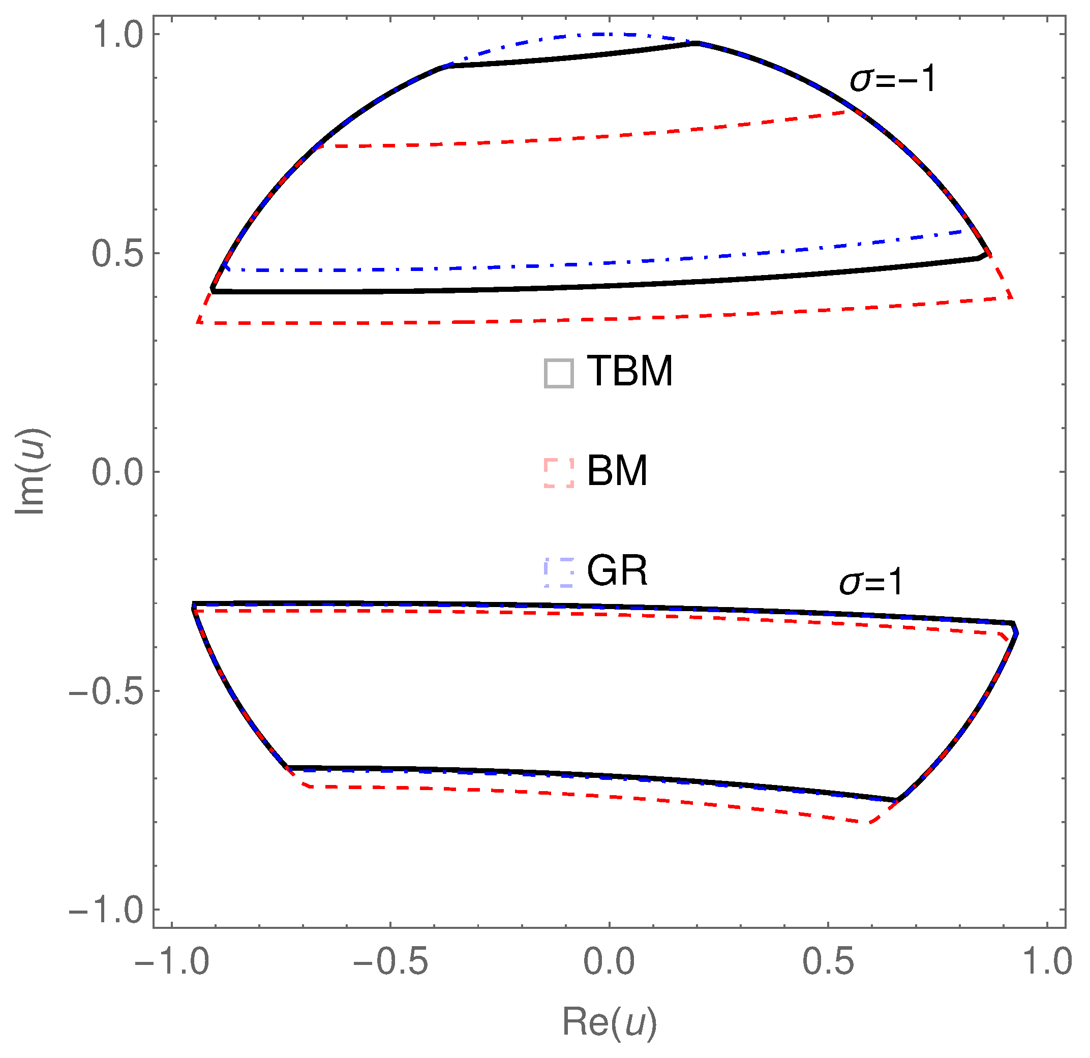
To find the set of values of Re ( u ) , Im ( u ) that allows us to reproduce the best-fit point of J CP ( J CP b f ), in Figure 2, we plot the ensemble of u values which makes the modified versions of TBM (black solid line), BM (red dashed line) and GR (blue dot-dashed line) compatible with J CP bf at 1 σ , subject to the constraint | u | < 1 . Given the similarities in the analytical structure of TBM, BM and GR, we see that the overlapping complex u-region is covered; in addition, as commented above, we also expect a less relevant dependence on Re ( u ) compared to Im ( u ) .
The main conclusion is that | Im ( u ) | 0.3 (and almost any Re ( u ) in the [ 1 , 1 ] range) is enough to obtain the correct amount of leptonic CP violation, for any choice of the starting matrix. The mild Re ( u ) , Im ( u ) correlation is mainly dictated by the constraint | u | < 1 .
Now, we target for the expressions of the mixing angles. For the reactor angle, we obtain a formula which is independent on the θ ˜ 12 parameter (and thus, on the sign of σ ) up to 𝒪 ( λ 3 ) terms (notice that 𝒪 ( λ 2 ) terms vanish):
sin ( θ 13 ) = 1 / 2 + | u | 2 + 2 Re ( u ) λ + 2 2 A ρ 4 A η Im u + ( 2 + 4 A ρ ) Re ( u ) | u | 2 ( 3 2 + 2 Re ( u ) ) 4 1 + 2 | u | 2 + 2 2 Re ( u ) λ 3 .
In the limit of exact TBM, BM and GR mixing ( u = 0 ), we recover the well-known relation sin ( θ 13 ) = λ 2 + 𝒪 ( λ 3 ) , which is still a good approximation (see also Table 2). Moreover, Equation (22) shows that, barring accidental cancellations, negative Re ( u ) values are needed to compensate for positive shifts driven by | u | (unless Im ( u ) is also small, in that case small positive values of Re ( u ) are also allowed).
Not too much must be said for the atmospheric angle; up to 𝒪 ( λ 3 ) , we obtain
tan ( θ 23 ) = 1 + λ 2 2 1 + 4 A 2 2 Re ( u ) .
The most interesting feature is the absence of any dependence on Im ( u ) ; thus, the small deviations from maximality are governed, besides the Cabibbo angle, by Re ( u ) only. We also have to mention that the current best-fit point is away from maximal mixing at the level of 3 σ (see Table 3). Thus, relatively large positive Re ( u ) are needed to shift tan ( θ 23 ) towards its 1 σ preferred value, which lies around tan ( θ 23 ) b f 0.9 . As in the previous case, no dependence on θ ˜ 12 appears so that exact TBM, BM and GR hypotheses give the same expression in Equation (23) with Re ( u ) = 0 .
Finally, for the solar angle, we obtain
tan ( θ 12 ) = tan ( θ ˜ 12 ) + λ 2 c ˜ 12 2 σ + λ 2 2 c ˜ 12 3 s ˜ 12 + + λ 3 4 c ˜ 12 4 σ 2 ( 1 2 A c ˜ 12 2 ρ ) + c ˜ 12 2 ( 2 | u | 2 + 2 Re ( u ) ) .
The most considerable feature is that the corrections implied by U 13 of Equation (17) are too small to be significant; thus, the expressions of θ 12 are very similar to those quoted in Table 2. In addition, once we specify the values of θ ˜ 12 for the relevant patterns, there are no free parameters up to 𝒪 ( λ 2 ) ; we can then derive the following sum-rules among physical angles that, for the sake of simplicity, we report here up to the first order in sin ( θ 13 ) :
tan ( θ 12 ) = 1 2 + 3 σ sin ( θ 13 ) / 2 for TBM 1 + 2 σ sin ( θ 13 ) for BM 2 5 / ( 5 + 5 ) + 10 σ sin ( θ 13 ) / ( 5 + 5 ) for GR .
The only possibility to (marginally) reconcile the previous sum rules with the experimental value happens for BM mixing with σ = 1 , which shows a deviation from tan ( θ 12 ) b f at around 3 % (compare with Figure 1); for the other mixing patterns, this difference amounts to values as large as ∼20% for GR and ∼30% for TBM. To better quantify the (dis-)agreements of the obtained U PMNS with the experimental data after including the corrections in Equation (17), we perform a simple χ 2 test, with the following function:
χ 2 = J CP J CP b f 2 σ J CP 2 + sin ( θ 13 ) sin ( θ 13 ) b f 2 σ sin ( θ 13 ) 2 + tan ( θ 23 ) tan ( θ 23 ) b f 2 σ tan ( θ 23 ) 2 + tan ( θ 12 ) tan ( θ 12 ) b f 2 σ tan ( θ 12 ) 2
For all patterns, the minimum of the χ 2 is very large, in the range (10–103) and it is dominated by the tan ( θ 12 ) term; in fact, if we exclude θ 12 from the χ 2 function, the fit improves considerably for all patterns, with χ m i n 2 𝒪 ( 20 ) (the best performance being the one obtained by BM mixing with σ = 1 ). The problem related to the deviation from the maximality of θ 23 is, instead, less relevant because of a larger relative 1 σ error compared to θ 12 . Finally, the corrections analyzed here help in improving the values of Δ , Δ = ( 2708 , 2492 , 2573 ) for TBM, BM and GR mixing, respectively. Obviously, assuming for the variable u a smaller value, that is shifting u λ N u , does not solve the problem for any integer N.

2.3. Perturbation on the (23)-Sector

One possibility to alleviate the problem in the (23)-sector is to slightly modify U 23 of Equation (4) by inserting a new real parameter ω according to3
U 23 = 1 0 0 0 1 2 λ ω 2 λ 2 ω 2 2 λ 3 ω 3 1 2 + ω λ 0 1 2 ω λ 1 2 λ ω 2 λ 2 ω 2 2 λ 3 ω 3 .
Notice that, to maintain the unitarity of U 23 , we displayed up to 𝒪 ( λ 3 ) terms. We repeat the same calculations as before and indicate with a prime the new expressions of the mixing parameters while leaving unprimed the results of the previous section. The relevant corrections driven by ω are as follows:
J CP = J CP λ 3 2 Im ( u ) ω cos 2 θ ˜ 12 + 2 σ ω 2 sin 2 θ ˜ 12 sin ( θ 13 ) = sin ( θ 13 ) + λ 2 ω 2 2 + 2 Re ( u ) 1 + 2 | u | 2 + 2 2 Re ( u ) tan ( θ 23 ) = tan ( θ 23 ) + 2 2 λ ω tan ( θ 12 ) = tan ( θ 12 ) λ 2 ω σ cos 2 θ ˜ 12 .
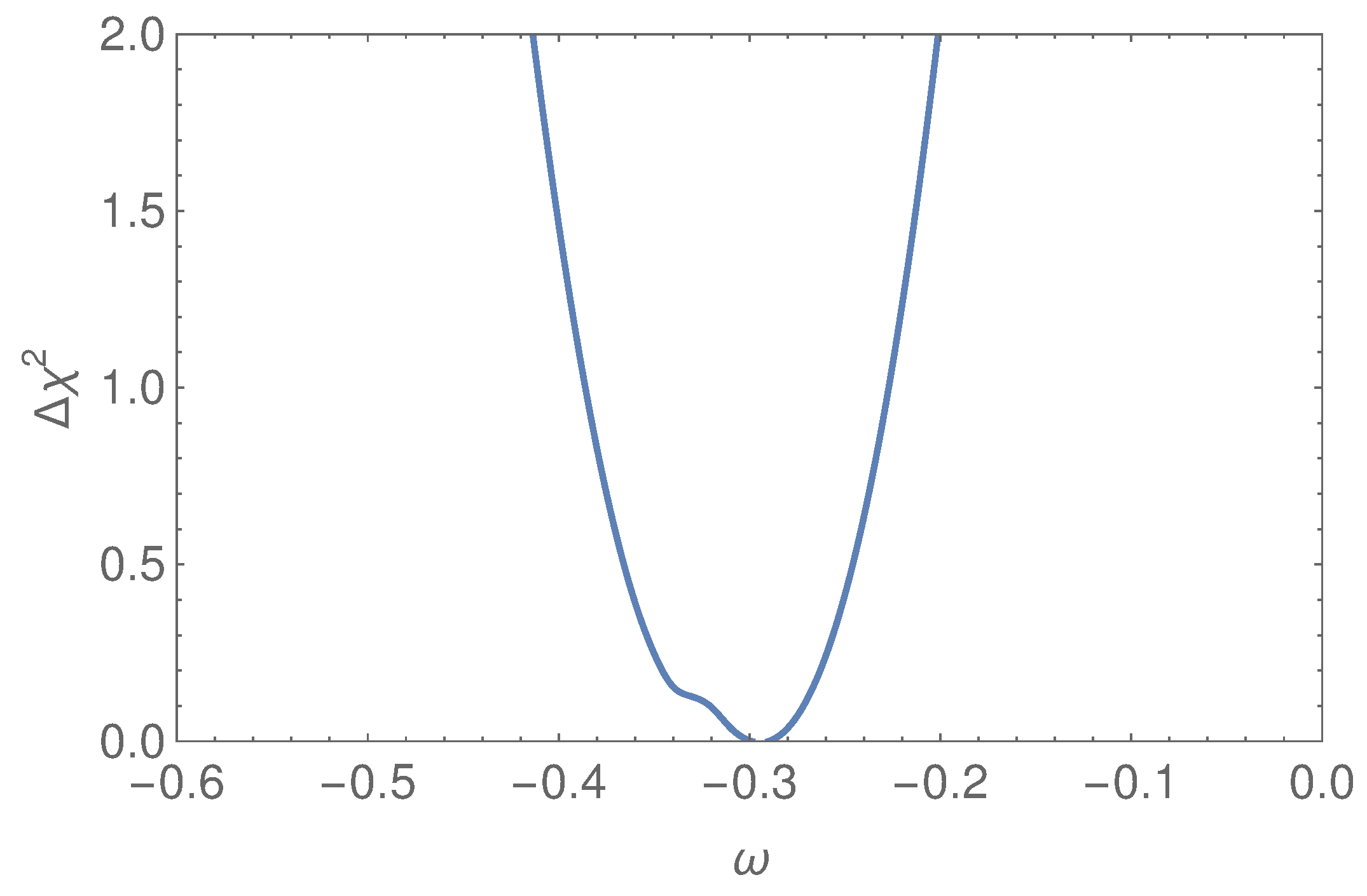
We see that J CP , θ 12 and θ 13 acquire small 𝒪 ( λ 2 3 ) corrections that do not improve the fit compared to the previous section. For the atmospheric angle, instead, an 𝒪 ( λ ) is relevant, especially for negative values of ω as, starting from maximality, we need a negative correction to jump into the experimental value4. Notice that this is true for any value of σ . However, even though the atmospheric angle turns out to be in the correct range, the fits to the expressions in Equation (28) are only slightly improved but still remain 𝒪 ( 100 ) because of the poor foreseen solar angle; as before, only the modified BM mixing case presents a good minimum of the χ 2 at χ m i n 2 = 3.47 . For the sake of illustration, the behavior of the Δ χ 2 = χ 2 χ m i n 2 as a function of ω is presented in Figure 3. For every ω , we have marginalized over Re ( u ) and Im ( u ) in the fit.

2.4. The Full Glory: Perturbation on the (12)-Sector

The results of the previous sections have shown that the predictions for J CP and sin ( θ 13 ) are good for all mixing once the u-corrections are included. The ω corrections are needed to reconcile the θ 23 deviations from maximal mixing (common to all patterns), while the solar angle remains sensitively away from its experimental value for TBM and GR mixing but sufficiently close to it for BM. Thus, in order to complete our program to match the data of Table 3, we need to add a (real) correction of 𝒪 ( λ ) to the (12)-sector that we dub with z. We parameterize it in the following way:
U 12 = K s ˜ 12 σ + z λ 0 s ˜ 12 σ z λ K 0 0 0 1 ,
where K = c ˜ 12 s ˜ 12 z σ / c ˜ 12 λ z 2 / ( 2 c ˜ 12 3 ) λ 2 s ˜ 12 z 3 σ / ( 2 c ˜ 12 5 ) λ 3 . The expression of the mixing parameters are modified accordingly; in particular, θ 13 and θ 23 are unaffected by z, so their expressions of Equation (28) are valid even in this case. The Jarlskog invariant obtains an 𝒪 ( λ 2 ) correction of the form
J CP = J CP + λ 2 2 cos ( 2 θ ˜ 12 ) Im ( u ) cos ( θ ˜ 12 ) z .
By construction, the most interesting case is related to θ 12 ; here, corrections of 𝒪 ( λ ) driven by z compete with that shown in Equation (24):
tan ( θ 12 ) = tan ( θ 12 ) + λ σ z cos 3 θ ˜ 12 .
Thus, we expect that a cancellation among the λ coefficients could bring the TBM and GR mixing in agreement with the data (for any σ ), while for BM, the contribution from z (and σ = 1 ) must be small in order to not destroy the agreement found above; conversely, we expect that σ = 1 will be acceptable for non-vanishing z corrections. To check whether this is the case, we minimized the χ 2 function of Equation (26) over the four independent parameters Re ( u ) , Im ( u ) , ω and z and reported their best-fit values in Table 4.
For all patterns, the minimum of the χ 2 is very close to zero, so we did not report it on the table. As expected, the magnitude and signs of the needed z s reflects our considerations below Equation (31). In addition, the very similar values for Re ( u ) and Im ( u ) can be understood from Figure 2, where the acceptable regions for such parameters are almost equivalent for each pattern. Finally, compared to the previous section, the value of ω is compatible with the BM case previously analyzed and, as expected, tends to assume a very similar strength for all other patterns and signs of σ ( 𝒪 ( λ ) corrections are universal). The 90% and 99% confidence levels of the χ 2 function in the ( ω , z ) -plane for TBM (left panel), BM (middle panel) and GR (right panel) are reported in Figure 4; in each plot, we included both ± 1 possibilities for σ and marginalized over the ( Re ( u ) , Im ( u ) ) ) pair.

3. On the Neutrino Masses

The next step is to ensure that our procedure is able to reproduce the solar and atmospheric mass differences. Equation (5) offers the structure of the neutrino mixing matrix in terms of a right rotation U R (four real parameters), three right-handed neutrino masses and three Dirac neutrino masses, for a total of ten unknown parameters; of those, four have been used to constrain the matrix T in Equation (6), and the remaining six parameters are left to describe neutrino masses. To determine them, one can try to figure out the structure of the diagonal matrix S by inverting Equation (6), so that
S = T m ν D d i a g U R ( M R d i a g ) 1 U R m ν D d i a g T .
Notice that the matrix S m ν d i a g does not depend on the quark mixing. One possibility to determine the unknown parameters is to rephrase Equation (32) to the more useful form:
S T m 0 T = 0 .
Its left-hand side is a symmetric matrix made complex by the entries of m ν d i a g and by the T matrix, needed to successfully reproduce the leptonic CP violation. Thus, Equation (33) is equivalent to 12 conditions, which have to be simultaneously valid. However, we can easily verify that the imaginary parts of the elements of T are always smaller than the real part (at the level of 20% or smaller) with a notable exception of element (13), for which the imaginary part is either larger (in the only case when T is the corrected BM mixing with σ = 1 ) or just half of the real part. With the aim of catching the relevant physics, not obfuscated by useless details (phases are of the uttermost importance for CP violation, not for neutrino masses), we prefer to deal with real S and T matrices; this allows us to reduce the number of constraints to only six5. Even in this case, the large number of free parameters makes the expressions of neutrino masses quite cumbersome. Thus, we only give a numerical solution to Equation (33). For the S matrix, we take the following expression, valid for the Normal Ordering (NO) case:
S = diag ( m 1 , m 1 2 + Δ m s o l 2 , m 1 2 + Δ m a t m 2 ) ,
where m 1 is the absolute neutrino mass scale that, for the sake of simplicity, we assume vanishing. We then construct the adimensional function:
F ( m ν D , M R , θ R ) = j < i = 1 3 S i j ( T T m 0 T ) i j 2 Δ m sol 2 ,
and look for minima as close as possible to zero. Here, the vectors have the following entries with obvious meaning:
m ν D = m ν D 1 , m ν D 2 , m ν D 3 M R = M R 1 , M R 2 , M R 3 θ R = θ R 12 , θ R 13 , θ R 23 .
We consider ourselves satisfied when F ( m ν D , M R , θ R ) < 1 , meaning that all the differences between the corresponding matrix elements of S and T T m 0 T are smaller than the smallest measured mass scale Δ m sol 2 . The minimization procedure has been carried out by means of the software MultiNest v 3.10, which is based on nested sampling normally used for calculation of the Bayesian evidence [40,41,42]. The choice of priors in this context is relevant. To prove that a solution to the system (33) exists, we set
1 m ν D 1 / G e V < 10 , 10 m ν D 2 / G e V < 100 , 100 m ν D 3 / G e V < 500 , 10 13 M R 1 / G e V < 10 14 , 10 14 M R 2 / G e V < 10 15 , 10 15 M R 3 / G e V < 10 16 , m ν D 1 / G e V < 10 , θ R [ 0 , 2 π ) . 100 m ν D 3 / G e V < 500
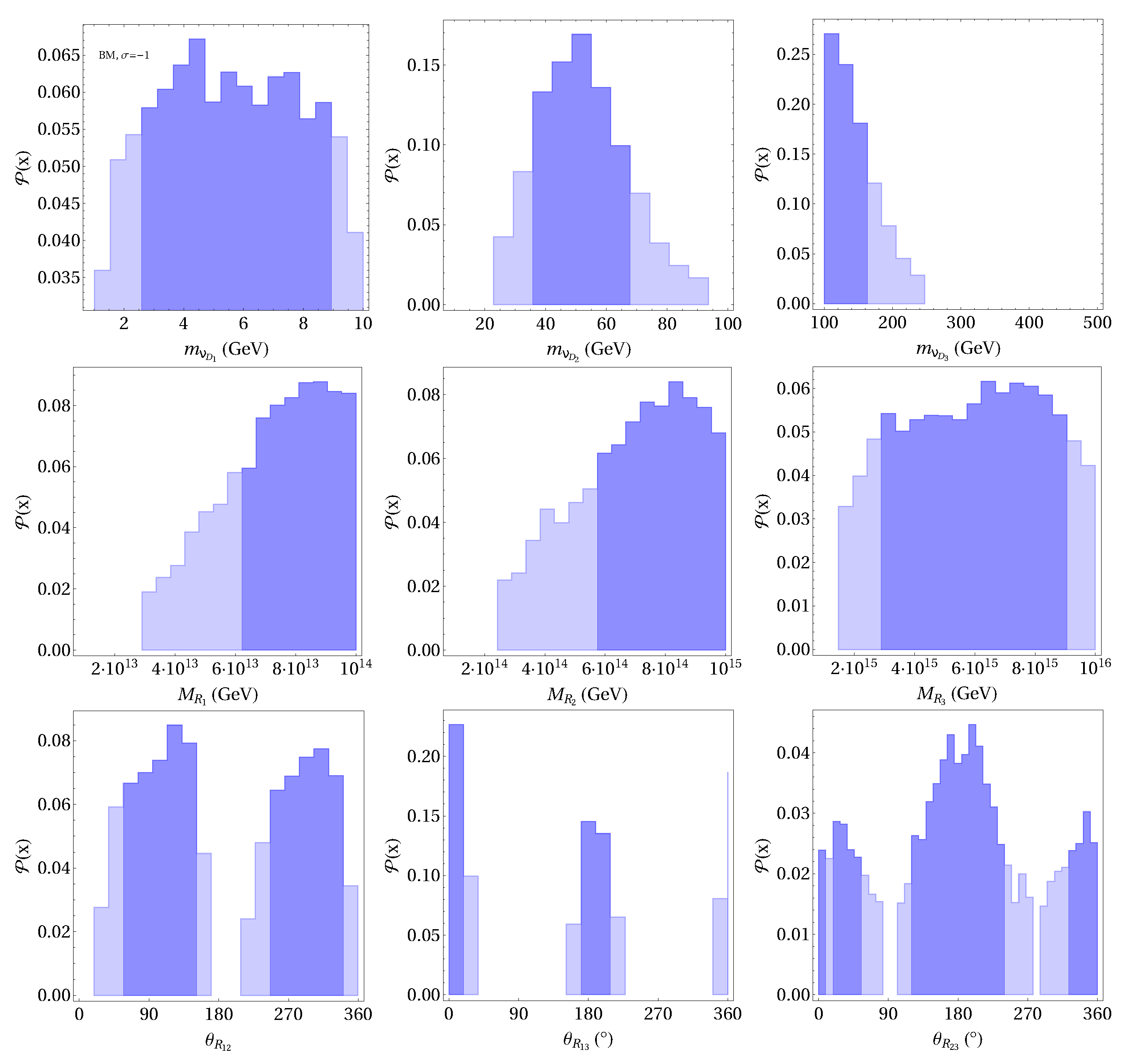
Notice that, with the neutrino masses given by complicated expressions of parameters, the positions m ν D 1 < m ν D 2 < m ν D 3 and M R 1 < M R 2 < M R 3 do not correspond a priori to a definite mass hierarchy, as it would be the case for a standard see-saw mechanism, where, for example, m i m ν D i 2 / M R i for NO. We have analyzed the six different cases corresponding to modified BM, TBM and GR and the two values of σ = ± 1 ; for each texture, we reported in Table 5 the minimum of F ( m ν D , M R , θ R ) and the values of the vectors m ν D , M R and θ R in which the minimum is assumed. We also report in Figure 5 an example of posterior distributions for the BM case, σ = 1 (all cases are very similar to each other).
Let us further analyze in detail the results of our minimizing procedure. First of all, none of the analyzed patterns can be tagged as a preferred one, as the minima of the F function are very close to each other. This is in agreement with what we found for the mixing angles where, after including all relevant corrections, no preferred choice emerged. The vector m ν D is characterized by the fact that the first and third elements prefer values at their upper and lower limits, respectively, while m ν D 2 is generally confined in the central region (with an exception for the case TBM, σ = + 1 , which, instead, prefers larger values). As for the Majorana masses, we observe similarities in all elements among the different patterns: M R 1 and M R 3 tend to stay close to their allowed lower and upper bounds, respectively, while M R 2 is mostly concentrated in the middle region around [40–90] · 10 13 GeV. It is interesting to observe that the posterior distributions (middle panels of Figure 5) are almost flat for M R 3 but peaked at large allowed values for M R 1 and M R 2 . While for the latter case this seems consistent with the values at the minimum of F, for the former, this behavior does not completely match what reported in Table 5. We interpret this as that M R 1 gives a smaller contribution to F as the other Majorana masses. This also happens for the first Dirac neutrino mass m ν D 1 , whose best-fit value is close to its upper limit while the posterior distribution is essentially flat. Finally, a look at Figure 5 reveals that the posterior distributions for the mixing angles are multi-modal; in particular, a clear bi-modal distribution is seen for θ R 12 , around | sin ( θ R 12 ) | 1 / 2 , and for θ R 13 around | sin ( θ R 13 ) | 0 ; this is also visible in Table 5. A less clear bi-modal behavior is also present for θ R 23 , but the spreads around the maximum posterior probability are not negligible. Assuming the fixed values sin ( θ R 12 ) = 1 / 2 and sin ( θ R 13 ) = 0 , the right-handed rotation implied by our fit is as follows:
U R = 3 / 2 1 / 2 0 c 23 / 2 3 c 23 / 2 s 23 s 23 / 2 3 s 23 / 2 c 23 .

4. Conclusions

In this paper, we have investigated in detail the hypothesis that the PMNS mixing matrix is given by the relation U P M N S = V C K M T , where T is a unitary matrix. By considering the decomposition T U 23 U 13 U 12 , we have shown that a T matrix coinciding with TBM, BM and GR mixing fails, among others, to reproduce the experimental preferred value of the Jarlskog invariant, which is related to the third power of the Cabibbo angle. To solve these issues, we have analyzed 𝒪 ( λ ) corrections to the U i j matrices, showing that a complex parameter u is needed in the (13) rotation to reconcile our ansatz with the experimental amount of leptonic CP violation. While a correction ω in the (23)-sector is needed for a substantial deviation of the atmospheric angle from maximality, it only marginally improves the global fit to the experimental values of the mixing angles because of a wrong estimate of θ 12 in all cases but BM. Thus, a shift in the (12) plane is mandatory to account for the solar angle and, consequently, to obtain an excellent fit for all mixing parameters and for any initial choice of T. The ansatz illustrated here is also appropriate to reproduce the value of solar and atmospheric mass differences. Indeed, equipped with the best-fit values of the Re ( u ) , Im ( u ) , ω and z parameters, we have shown that a description of neutrino masses via the see-saw mechanism is possible. Because of the cumbersome analytical expressions of Δ m s o l , a t m 2 , we relied on a numerical scan of the vector components of m ν D , M R and θ R of Equation (36) and found that, with our choice of priors, a complete description of neutrino masses and mixing under the assumption U P M N S = V C K M T is possible.
The analysis shown here can be further extended to contemplate different starting ansatzs whose structures are different from those analyzed here; an example in this direction is offered by the trimaximal mixing [43], which differs from the BM structure in predicting sin ( θ 13 ) = 1 / 3 .

Author Contributions

Conceptualization, A.G., S.M. and D.M.; Methodology, A.G., S.M. and D.M.; Software, A.G., S.M. and D.M.; Validation, A.G., S.M. and D.M.; Formal Analysis, A.G., S.M. and D.M.; Investigation, A.G., S.M. and D.M.; Resources, A.G., S.M. and D.M.; Data Curation, A.G., S.M. and D.M.; Writing—Original Draft Preparation, A.G., S.M. and D.M.; Writing—Review & Editing, A.G., S.M. and D.M.; Visualization, A.G., S.M. and D.M.; Supervision, A.G., S.M. and D.M.; Project Administration, A.G., S.M. and D.M.; Funding Acquisition, A.G., S.M. and D.M. All authors have read and agreed to the published version of the manuscript.

Funding

This research received no external funding.

Data Availability Statement

The data presented in this study are openly available in https://inspirehep.net/literature/2803966, https://arxiv.org/abs/2407.02487 (accessed on 11 August 2024).

Acknowledgments

We thank João Penedo and Matteo Parriciatu for useful comments and suggestions on our manuscript.

Conflicts of Interest

Authors declare no conflict of interest.

Appendix A. Full 𝒪 (λ3) Formulae

For the sake of completeness, we report here the full 𝒪 ( λ 3 ) expressions of the mixing parameters obtained from our ansatz U P M N S = V C K M T .
J = λ 4 σ Im ( u ) sin ( 2 θ ˜ 12 ) + λ 2 Im ( u ) cos 2 ( θ ˜ 12 ) 4 cos ( θ ˜ 12 ) 2 cos ( θ ˜ 12 ) + 2 z + λ 3 8 σ sin ( 2 θ ˜ 12 ) 2 A η + 2 Im ( u ) 2 + | u | 2 + 2 Re ( u ) + λ 3 2 Im ( u ) ω cos 2 θ ˜ 12 + 2 σ ω 2 sin 2 θ ˜ 12 + λ 3 z σ 8 2 sin ( θ ˜ 12 ) Im ( u ) + 2 z Im ( u ) sin ( θ ˜ 12 ) cos ( θ ˜ 12 ) 3 3 cos 2 ( θ ˜ 12 ) + sin 2 ( θ ˜ 12 )
sin ( θ 13 ) = 1 / 2 + | u | 2 + 2 Re ( u ) λ + + λ 2 ω 2 2 + 2 Re ( u ) 1 + 2 | u | 2 + 2 2 Re ( u ) + + λ 3 2 2 A ρ 4 A η Im u + ( 2 + 4 A ρ ) Re ( u ) | u | 2 ( 3 2 + 2 Re ( u ) ) 4 1 + 2 | u | 2 + 2 2 Re ( u ) + + λ 3 ω 2 2 Im 2 ( u ) 2 Re ( u ) u ) Re ( u ) + 2 + 2 Im 2 ( u ) + 1 3 / 2
tan ( θ 23 ) = 1 + 2 2 λ ω + λ 2 2 1 + 4 A 2 2 Re ( u ) + + λ 3 ω 4 2 A 2 Re ( u ) + 12 2 ω 2 2 + 2 ( ) u ) ) 4 1 + 2 | u | 2 + 2 2
tan ( θ 12 ) = tan ( θ ˜ 12 ) + λ σ 2 c ˜ 12 + 2 z 2 c ˜ 12 3 + λ 2 2 c ˜ 12 3 s ˜ 12 λ 2 ω σ c ˜ 12 2 + λ 2 z 2 s ˜ 12 c ˜ 12 4 + 3 λ 2 z 2 s ˜ 12 2 c ˜ 12 5 + + λ 3 4 c ˜ 12 4 σ 2 ( 1 2 A c ˜ 12 2 ρ ) + c ˜ 12 2 ( 2 | u | 2 + 2 Re ( u ) ) + + λ 3 2 c ˜ 12 7 2 2 c ˜ 12 4 ω ( c ˜ 12 σ ω + s ˜ 12 ) + c ˜ 12 2 z c ˜ 12 2 σ 2 ω sin ( 2 θ ˜ 12 ) + 3 σ s ˜ 12 2 + c ˜ 12 σ z 2 ( 5 3 cos ( 2 θ ˜ 12 ) ) 2 + σ z 3 ( 3 2 cos ( 2 θ ˜ 12 ) )

Notes

1
For our purposes, it is enough to consider the normal hierarchy only, as the only significant difference with respect to the inverted ordering case is a slight preference for the opposite θ 23 octant.
2
We do not report the spread of J CP as, for any pattern, its absolute value is around two orders of magnitude smaller than the experimental best-fit.
3
Since the complex variable u was already enough to guarantee the correct amount of leptonic CP violation, we prefer to reduce the number of free parameters by choosing a real correction ω .
4
The three main neutrino global fits [33,38,39] do not agree on the preferred θ 23 octant, even though the 3 σ ranges are all compatible. In our analysis, a higher octant value for θ 23 can be easily obtained with a positive ω value.
5
If, instead, we prefer to deal with complex matrices, phases must thus be added to U R to help in vanishing all imaginary parts of Equation (33).

References

  1. Minakata, H.; Smirnov, A.Y. Neutrino mixing and quark-lepton complementarity. Phys. Rev. D 2004, 70, 073009. [Google Scholar] [CrossRef]
  2. Georgi, H.; Jarlskog, C. A New Lepton-Quark Mass Relation in a Unified Theory. Phys. Lett. B 1979, 86, 297–300. [Google Scholar] [CrossRef]
  3. Raidal, M. Relation Between the Neutrino and Quark Mixing Angles and Grand Unification. Phys. Rev. Lett. 2004, 93, 161801. [Google Scholar] [CrossRef] [PubMed]
  4. Frampton, P.H.; Mohapatra, R.N. Possible Gauge Theoretic Origin for Quark-Lepton Complementarity. J. High Energy Phys. 2005, 2005, 025. [Google Scholar] [CrossRef]
  5. Antusch, S.; King, S.; Mohapatra, R. Quark–lepton complementarity in unified theories. Phys. Lett. B 2005, 618, 150–161. [Google Scholar] [CrossRef]
  6. Xing, Z.Z. Nontrivial correlation between the CKM and MNS matrices. Phys. Lett. B 2005, 618, 141–149. [Google Scholar] [CrossRef]
  7. Datta, A.; Everett, L.; Ramond, P. Cabibbo haze in lepton mixing. Phys. Lett. B 2005, 620, 42–51. [Google Scholar] [CrossRef]
  8. Patel, K.M. An SO(10)XS4 Model of Quark-Lepton Complementarity. Phys. Lett. B 2011, 695, 225–230. [Google Scholar] [CrossRef]
  9. Picariello, M.; Chauhan, B.C.; Pulido, J.; Torrente-Lujan, E. Predictions from non-trivial quark-lepton complementarity. Int. J. Mod. Phys. A 2007, 22, 5860–5874. [Google Scholar] [CrossRef]
  10. Chauhan, B.; Picariello, M.; Pulido, J.; Torrente-Lujan, E. Quark–lepton complementarity with lepton and quark mixing data predict θ 13 PMNS = ( 9 2 + 1 ) ° . Eur. Phys. J. C 2007, 50, 573–578. [Google Scholar] [CrossRef]
  11. Harada, J. Neutrino mixing and CP violation from Dirac-Majorana bimaximal mixture and quark-lepton unification. Europhys. Lett. (EPL) 2006, 75, 248–253. [Google Scholar] [CrossRef]
  12. Zhukovsky, K.; Davydova, A.A. CP violation and quark-lepton complementarity of the neutrino mixing matrix. Eur. Phys. J. C 2019, 79, 385. [Google Scholar] [CrossRef]
  13. Zhang, Y.; Zhang, X.; Ma, B.Q. Quark-lepton complementarity and self-complementarity in different schemes. Phys. Rev. D 2012, 86, 093019. [Google Scholar] [CrossRef]
  14. Zhang, X.; Zheng, Y.j.; Ma, B.Q. Quark-lepton complementarity revisited. Phys. Rev. D 2012, 85, 097301. [Google Scholar] [CrossRef]
  15. Barranco, J.; Gonzalez Canales, F.; Mondragon, A. Universal Mass Texture, CP violation and Quark-Lepton Complementarity. Phys. Rev. D 2010, 82, 073010. [Google Scholar] [CrossRef]
  16. Cheung, K.; Kang, S.K.; Kim, C.S.; Lee, J. Lepton flavor violation as a probe of quark-lepton unification. Phys. Rev. D 2005, 72, 036003. [Google Scholar] [CrossRef]
  17. Hochmuth, K.A.; Rodejohann, W. Low and high energy phenomenology of quark-lepton complementarity scenarios. Phys. Rev. D 2007, 75, 073001. [Google Scholar] [CrossRef]
  18. Plentinger, F.; Seidl, G.; Winter, W. The Seesaw mechanism in quark-lepton complementarity. Phys. Rev. D 2007, 76, 113003. [Google Scholar] [CrossRef]
  19. Kang, S.K. Revisiting the Quark-Lepton Complementarity and Triminimal Parametrization of Neutrino Mixing Matrix. Phys. Rev. D 2011, 83, 097301. [Google Scholar] [CrossRef]
  20. Ke, H.W.; Liu, T.; Li, X.Q. Determination of the mixing between active neutrinos and sterile neutrino through the quark-lepton complementarity and self-complementarity. Phys. Rev. D 2014, 90, 053009. [Google Scholar] [CrossRef]
  21. Ferrandis, J.; Pakvasa, S. Quark-lepton complenmentarity relation and neutrino mass hierarchy. Phys. Rev. D 2005, 71, 033004. [Google Scholar] [CrossRef]
  22. Kang, S.K.; Kim, C.; Lee, J. Importance of threshold corrections in quark–lepton complementarity. Phys. Lett. B 2005, 619, 129–135. [Google Scholar] [CrossRef]
  23. Schmidt, M.A.; Smirnov, A.Y. Quark Lepton Complementarity and Renormalization Group Effects. Phys. Rev. D 2006, 74, 113003. [Google Scholar] [CrossRef]
  24. Dighe, A.; Goswami, S.; Roy, P. Quark-lepton complementarity with quasidegenerate Majorana neutrinos. Phys. Rev. D 2006, 73, 071301. [Google Scholar] [CrossRef]
  25. Ferrandis, J.; Pakvasa, S. A Prediction for |U(e3)| from patterns in the charged lepton spectra. Phys. Lett. B 2004, 603, 184–188. [Google Scholar] [CrossRef]
  26. Meloni, D. Bimaximal mixing and large theta13 in a SUSY SU(5) model based on S4. J. High Energy Phys. 2011, 2011, 10. [Google Scholar] [CrossRef]
  27. Harada, J. Non-maximal θ23, large θ13 and tri-bimaximal θ12 via quark-lepton complementarity at next-to-leading order. Europhys. Lett. 2013, 103, 21001. [Google Scholar] [CrossRef]
  28. Sharma, G.; Chauhan, B.C. Quark-lepton complementarity predictions for θ 23 pmns and CP violation. J. High Energy Phys. 2016, 2016, 75. [Google Scholar] [CrossRef]
  29. Harrison, P.F.; Perkins, D.H.; Scott, W.G. Tri-bimaximal mixing and the neutrino oscillation data. Phys. Lett. B 2002, 530, 167. [Google Scholar] [CrossRef]
  30. Feruglio, F.; Paris, A. The golden ratio prediction for the solar angle from a natural model with A 5 flavour symmetry. J. High Energy Phys. 2011, 2011, 101. [Google Scholar] [CrossRef]
  31. Jarlskog, C. Commutator of the Quark Mass Matrices in the Standard Electroweak Model and a Measure of Maximal CP Nonconservation. Phys. Rev. Lett. 1985, 55, 1039–1042. [Google Scholar] [CrossRef] [PubMed]
  32. UTfit Collaboration; Bona, M.; Ciuchini, M.; Franco, E.; Lubicz, V.; Martinelli, G.; Parodi, F.; Pierini, M.; Roudeau, P.; Schiavi, C.; et al. The unitarity triangle fit in the standard model and hadronic parameters from lattice QCD: A reappraisal after the measurements of Δms and BR(Bτυτ). J. High Energy Phys. 2006, 2006, 081. [Google Scholar]
  33. Esteban, I.; Gonzalez-Garcia, M.C.; Maltoni, M.; Schwetz, T.; Zhou, A. The fate of hints: Updated global analysis of three-flavor neutrino oscillations. J. High Energy Phys. 2020, 2020, 178. [Google Scholar] [CrossRef]
  34. NuFIT 5.3. 2024. Available online: http://www.nu-fit.org/sites/default/files/v53.fig-chisq-dma.pdf (accessed on 11 August 2024).
  35. Abe, K. et al. [Super-Kamiokande Collaboration] Atmospheric neutrino oscillation analysis with external constraints in Super-Kamiokande I-IV. Phys. Rev. D 2018, 97, 072001. [Google Scholar] [CrossRef]
  36. Farzan, Y.; Smirnov, A.Y. Leptonic CP violation: Zero, maximal or between the two extremes. J. High Energy Phys. 2007, 2007, 59. [Google Scholar] [CrossRef]
  37. Altarelli, G.; Feruglio, F. Models of neutrino masses and mixings. New J. Phys. 2004, 6, 106. [Google Scholar] [CrossRef]
  38. de Salas, P.F.; Forero, D.V.; Gariazzo, S.; Martínez-Miravé, P.; Mena, O.; Ternes, C.A.; Tórtola, M.; Valle, J.W.F. 2020 global reassessment of the neutrino oscillation picture. J. High Energy Phys. 2021, 2021, 71. [Google Scholar] [CrossRef]
  39. Capozzi, F.; Di Valentino, E.; Lisi, E.; Marrone, A.; Melchiorri, A.; Palazzo, A. Unfinished fabric of the three neutrino paradigm. Phys. Rev. D 2021, 104, 083031. [Google Scholar] [CrossRef]
  40. Feroz, F.; Hobson, M.P. Multimodal nested sampling: An efficient and robust alternative to MCMC methods for astronomical data analysis. Mon. Not. R. Astron. Soc. 2008, 384, 449. [Google Scholar] [CrossRef]
  41. Feroz, F.; Hobson, M.P.; Bridges, M. MultiNest: An efficient and robust Bayesian inference tool for cosmology and particle physics. Mon. Not. R. Astron. Soc. 2009, 398, 1601–1614. [Google Scholar] [CrossRef]
  42. Feroz, F.; Hobson, M.P.; Cameron, E.; Pettitt, A.N. Importance Nested Sampling and the MultiNest Algorithm. Open J. Astrophys. 2019, 2, 10. [Google Scholar] [CrossRef]
  43. Harrison, P.F.; Perkins, D.H.; Scott, W.G. A Redetermination of the neutrino mass squared difference in tri-maximal mixing with terrestrial matter effects. Phys. Lett. B 1999, 458, 79–92. [Google Scholar] [CrossRef]
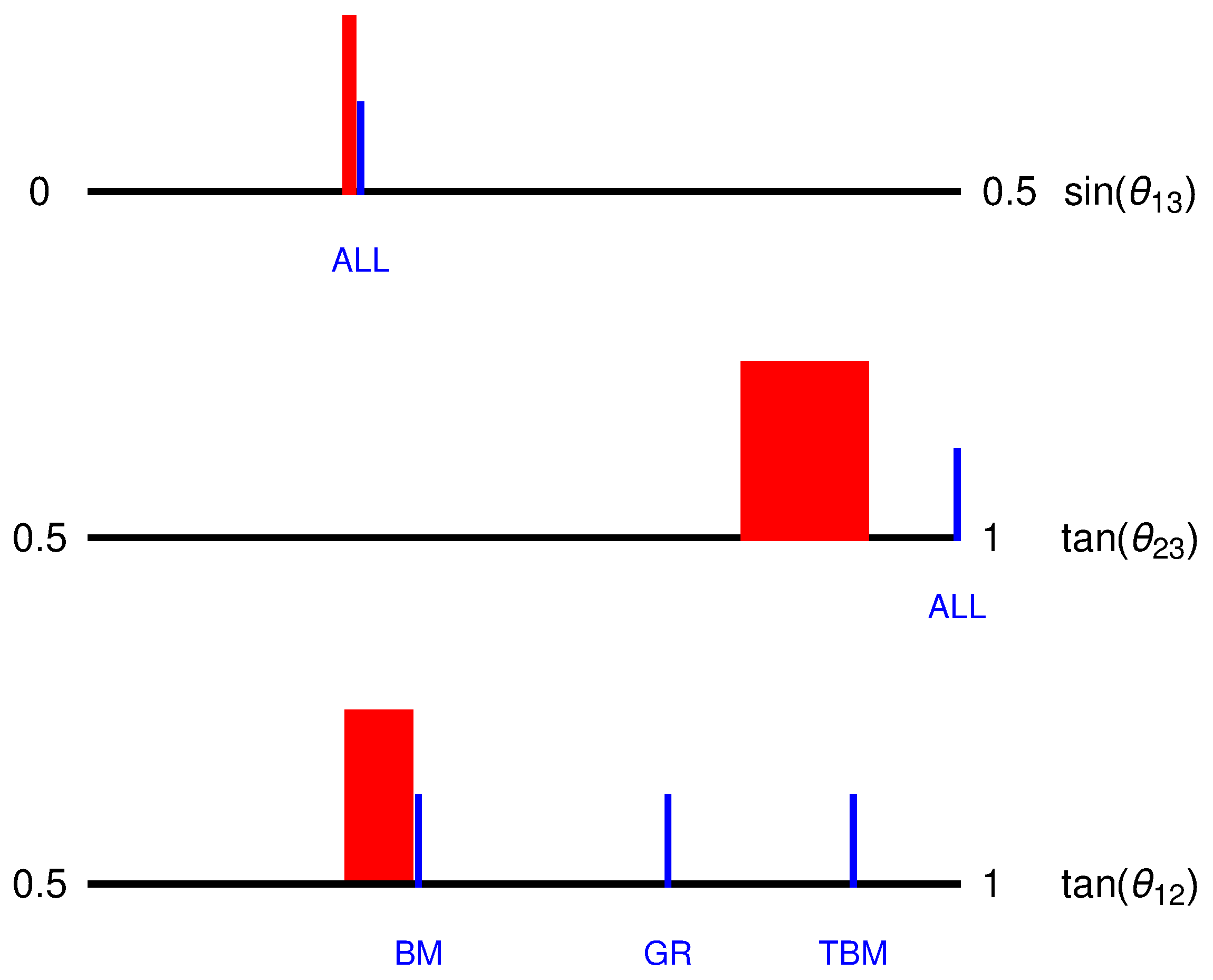
Figure 1. Current 2 σ experimental spread on tan ( θ 12 ) , tan ( θ 23 ) and sin ( θ 13 ) (red rectangles) and the predictions derived from U P M N S = V C K M T , where T can be TBM, BM and GR mixing patterns. Errors have been derived from Table 3.
Universe 10 00345 g001
Figure 2. Ensemble of u values which make the modified versions of TBM (black solid line), BM (red dashed line) and GR (blue dot-dashed line) compatible with J CP b f at 1 σ . The upper (lower) plots show the solutions obtained with σ = 1 ( σ = + 1 ).
Universe 10 00345 g002
Figure 3. Δ χ 2 = χ 2 χ m i n 2 behaviour as a function of ω for the modified BM mixing. In the fit procedure, we have marginalized over the ( Re ( u ) , Im ( u ) ) ) pair.
Universe 10 00345 g003
Figure 4. The 90% and 99% χ 2 confidence levels in the ( ω , z ) -plane for TBM (left panel), BM (middle panel) and GR (right panel). In each plot, we have reported both ± 1 possibilities for σ and marginalized over the ( Re ( u ) , Im ( u ) ) ) pair.
Universe 10 00345 g004
Figure 5. Posterior distributions for the elements of the vectors m ν D (first line) M R ; (middle line) and θ R (lower line) for the BM case, σ = 1 . Darker and lighter blue refer to 68% and 95% credible intervals, respectively.
Universe 10 00345 g005
Table 1. Best-fit value and 1 σ range of the V C K M parameters, from [32].
ParameterBest-Fit Value and 1 σ Range
λ 0.2251 ± 0.0008
A 0.828 ± 0.01
η 0.355 ± 0.009
ρ 0.164 ± 0.009
Table 2. Perturbative predictions on sin ( θ 13 ) , tan ( θ 12 ) , tan ( θ 23 ) (up to 𝒪 ( λ ) ) and J CP (up to 𝒪 ( λ 3 ) ) as obtained from the ansatz U P M N S = V C K M T , where T can be TBM, BM and GR mixing patterns. In the last column, we report the values of the variable Δ defined in Equation (16).
T sin ( θ 13 ) tan ( θ 12 ) tan ( θ 23 ) J CP Δ
U T B M λ 2 1 2 + 3 λ 2 2 1 1 6 A η λ 3 2715
U B M λ 2 1 2 λ 1 1 4 2 A η λ 3 2500
U G R λ 2 2 5 5 + 5 + 5 2 5 + 5 λ 1 1 2 10 A η λ 3 2580
Table 3. Neutrino observables and their 1 σ ranges as derived from NuFIT 5.3 [33,34], using the dataset with SK atmospheric data [35]. For the extraction of the best-fit value and 1 σ uncertainty of the Jarlskog invariant, we refer to its one-dimensional χ 2 projection from NuFIT 5.3.
ParameterBest-Fit Value and 1 σ Range
r Δ m sol 2 / | Δ m atm 2 | 0.0295 ± 0.0008
tan ( θ 12 ) 0.666 ± 0.019
sin ( θ 13 ) 0.149 ± 0.002
tan ( θ 23 ) 0.912 ± 0.035
J CP 0.027 ± 0.010
Table 4. Values of the parameters Re ( u ) , Im ( u ) , ω and z that minimize the χ 2 function of Equation (26), computed for σ = 1 and, in parenthesis, for σ = 1 . For all patterns, χ m i n 2 0 .
PatternRe ( u ) Im ( u ) ω z
TBM−0.27 (−0.27)0.57 (−0.55)−0.27 (−0.27)−0.50 (−0.77)
BM−0.27 (−0.29)0.57 (−0.56)−0.27 (−0.27)0.08 (−1.17)
GR−0.27 (−0.27)0.57 (−0.54)−0.27 (−0.27)−0.73 (−0.55)
Table 5. Results of the minimization procedure of the function F ( m ν D , M R , θ R ) in Equation (35). F m i n stands for the minimum value of such a function; the meaning of the three vectors m ν D , M R and θ R has been given in Equation (36).
F min m ν D (GeV) M R ( 10 13 GeV) θ R ( ° )
BM σ = + 1 0.42(9.35, 55.35, 117.70)(4.0, 70.10, 297.51)(145.80, 195.44, 162.01)
σ = 1 0.44(9.98, 36.84, 111.52)(3.59, 67.78, 708.16)(122.88, 12.88, 112.59)
TBM σ = + 1 0.31(9.38, 58.54, 130.56)(3.41, 93.21, 794.35)(331.00, 347.73, 317.70)
σ = 1 0.34(9.66, 34.52, 159.29)(2.09, 55.69, 485.30)(321.58, 354.03, 221.83)
GR σ = + 1 0.19(9.83, 80.88, 201.77)(3.55, 86.014, 728.73)(341.65, 171.70, 188.76)
σ = 1 0.45(9.26, 42.48, 156.88)(2.97, 38.95, 268.45)(145.00, 8.15, 341.63)
Disclaimer/Publisher’s Note: The statements, opinions and data contained in all publications are solely those of the individual author(s) and contributor(s) and not of MDPI and/or the editor(s). MDPI and/or the editor(s) disclaim responsibility for any injury to people or property resulting from any ideas, methods, instructions or products referred to in the content.