Using the Difference of the Inclinations of a Pair of Counter-Orbiting Satellites to Measure the Lense–Thirring Effect

Abstract

Let two test particles A and B, revolving about a spinning primary along ideally identical orbits in opposite directions, be considered. From the general expressions of the precessions of the orbital inclination induced by the post-Newtonian gravitomagnetic and Newtonian quadrupolar fields of the central object, it turns out that the Lense–Thirring inclination rates of A and B are equal and opposite, while the Newtonian ones oblateness are identical, due to the primary’s oblateness. Thus, the differences in the inclination shifts of the two orbiters would allow, in principle, for the classical effects to be cancelled out by enhancing the general relativistic ones. The conditions affecting the orbital configurations that must be satisfied for this to occur and possible observable consequences regarding the Earth are investigated. In particular, a scenario involving two spacecraft in polar orbits, branded POLAr RElativity Satellites (POLARES) and reminiscent of an earlier proposal by Van Patten and Everitt in the mid-1970s, is considered. A comparison with the ongoing experiment with the LAser GEOdynamics Satellite (LAGEOS) and LAser RElativity Satellite (LARES) 2 is made.

1. Introduction

For the first post-Newtonian (1pN) order, the General Theory of Relativity (GTR) predicts, among other things, that the orbital motion of a test particle freely orbiting a massive primary undergoes certain long-term, cumulative perturbations due to the gravitomagnetic field of the central object caused by its spin angular momentum. This is called the Lense–Thirring (LT) effect [1,2], although recent historical studies [3,4,5] have pointed out that it would be more correct to rename it the Einstein–Thirring–Lense effect. Essentially, it consists of variations in the orientation of both the orbital plane and in the orbit within the orbital plane itself, which manifest themselves cumulatively revolution after revolution. The shape and the size of the path are left unaffected, along with the time of passage at the pericentre. The LT effect is quite small in ordinary weak-field and slow-motion scenarios like in the surroundings of, say, the Earth or the Sun. Suffice it to say that the perihelion of Mercury, whose orbital period amounts to about 88 days, is shifted by the solar angular momentum by just 2 milliarcseconds per century (mas cty⁻¹). Moreover, the orbital plane of the LAser GEOdynamics Satellite (LAGEOS) [6], revolving about the Earth in less than 4 h, precesses at a rate as little as a few tens of milliarcseconds per year (mas yr⁻¹) due to the terrestrial gravitomagnetic field. On the other hand, such a general relativistic feature of motion should play a decisive role in the intricate dynamics of accreting matter close to Kerr black holes [7]. For example, it should drive the relativistic jets emanating from the surroundings of the supermassive black holes lurking in the active nuclei of radio galaxies [8,9]. Furthermore, after an accretion disk is formed around a supermassive black hole, initially with a strong misalignment with respect to the spin of the latter, as a consequence of a tidal disruption event of a nearby passing star, the LT effect causes the former to precess at early times before it finally aligns with the hole’s equatorial plane, ending the precession [10,11,12]. Finally, it is believed to cause quasi-periodic oscillations in the X-ray flux of accreting compact objects [13,14]. In such extreme natural laboratories, the expected magnitude of the aforementioned LT-driven effects is large, and thus does not pose a challenge to their detection. Rather, it is the interpretation of these phenomena that is difficult because of a lot competing effects whose physical mechanisms are not yet understood with enough accuracy [14]. As a consequence, it is of the utmost importance to have accurate and reliable tests of the LT effect performed in better-known environments in order to extrapolate its validity to the aforementioned strong field scenarios as well.

A wealth of gravitomagnetic effects other than the LT one exist for all scales [15,16,17,18,19,20]. Among them, the Pugh–Schiff [21,22] precession of the spin axes of four gyroscopes carried onboard a drag-free spacecraft orbiting the spinning Earth was successfully measured with a $19\%$ accuracy [23,24] by the dedicated Gravity Probe B (GP-B) mission [25,26]. To date, it still remains the only undisputed test of a gravitomagnetic effect in the existing peer-reviewed literature.

Returning to the LT effect, tests of it performed in astronomical scenarios in the solar system are quite rare. At present, there are reports in the literature of experiments made with Mercury in the Sun’s field [27,28,29] and with the Juno probe [30] around Jupiter [31,32]. Although none of them are in disagreement with the predictions of GTR, the reported uncertainties and the correlations with other estimated parameters are large enough to make the obtained results inconclusive.

As far as the terrestrial field is concerned, attempts have been underway for almost 30 years [33] to measure the LT orbital precessions using some geodetic satellites [34] tracked with the Satellite Laser Ranging (SLR) technique [35]; for reviews, see, e.g., [36,37,38] and references therein. Although the pericenter is also impacted by the gravitomagnetic field, for 20 years now the focus has been on the nodes of some satellites of the LAGEOS family [37,39,40]. Such a choice is due to the fact that the node of a satellite is much less severely disturbed than the perigee by the competing non-gravitational accelerations [41,42,43,44,45]. In 1976, Van Patten and Everitt [46,47] proposed looking at the sum of the nodes of a pair of low-altitude, drag-free spacecraft moving in opposite directions along ideally identical circular orbits passing through the Earth’s poles. Indeed, while the LT precessions add up, the nominally much larger competing Newtonian node shifts due to the Earth’s quadrupole mass moment, which would act as a major source of systematic bias, cancelling out, in principle, such an orbital configuration. An essentially equivalent version of such an idea, which its promoters intended to allow for a $\simeq 1\%$ measurement of the LT effect, was put forth 10 years later by Ciufolini [48], who proposed the use of a pair of passive SLR satellites following ideally identical non-polar orbits whose inclinations to the Earth’s equator are displaced by 180°. Indeed, such a scenario is conceptually equivalent to the one by Van Patten and Everitt, apart from the technical details pertaining the tracking method and the mechanism of compensation of the non-gravitational perturbations, since the classical node precessions also cancel out in this case, while the LT ones add up. Ciufolini [48]’s idea came to fruition in the last years with the launch of the LAser RElativity Satellite (LARES) 2 [49] in July 2022, joining LAGEOS, which had already been in orbit for almost 50 years. Ciufolini and coworkers [49] claimed that it would be possible to perform an LT test with such satellites that was accurate to $\simeq 0.2\%$. Unfortunately, their actual orbital configurations are just different enough to not allow the cancellation of the classical precessions to a good enough level [50].

Here, the proposal of using a pair of counter-revolving satellites in polar orbits, collectively dubbed POLAr RElativity Satellites (POLARES), is reexamined by showing that it would ideally be possible to use not only the sum of their nodes but also the differences in their inclinations to extract the LT effect, reducing the biasing impact of the Earth’s oblateness to an acceptable level. In principle, should the orbits be sufficiently elliptical, the difference of the perigees could also be adopted [51]. However, this would likely force the use of expensive drag-free technologies to counterbalance the non-gravitational perturbations that the perigees of geodetic satellites are particularly sensitive to.

The following physical and orbital parameters will be used in the rest of the paper. Among the constants of nature, G is the Newtonian constant of gravitation and c is the speed of light in a vacuum. As far as the key physical parameters of the Earth are concerned, $\mathsf{\mu }:=GM$ is the standard gravitational parameter given by the product of G times the mass M, $\mathit{J}=J\widehat{\mathit{k}}$ is the spin angular momentum, $\widehat{\mathit{k}}$ is the spin axis, R is the mean equatorial radius, $J_2$ is the first even zonal harmonic coefficient of degree ℓ = 2 and order $m=0$ of the multipolar expansion of the geopotential accounting for deviations from spherical symmetry, and ${\rho }_{\mathrm{atm}}$ is the atmospheric density at a height. The relevant orbital parameters characterizing the satellite’s motion with reference to some Earth-centered inertial (ECI) reference frames are the semimajor axis a, the eccentricity e, the semilatus rectum $p:=a\left(1-e\right)$, the inclination of the orbital plane I, and the longitude of the ascending node $\Omega$. Furthermore, $n_{\mathrm{K}}:=\sqrt{\mathsf{\mu }/a^3}$ is the Keplerian mean motion.

This paper is organized as follows. In Section 2, the general expressions for the classical and relativistic rates of change of the inclination and the nodes, averaged over one orbital revolution and valid for an arbitrary orientation of the primary’s spin axis, are reviewed. Their consequences for counter-revolving satellites in polar orbits are discussed, with particular emphasis on the difference of the inclinations. The impact of the orbital injection errors on the difference of the inclinations and the sum of then nodes is the subject of Section 3. A comparison with LAGEOS and LARES 2 is made in Section 4. Section 5 summarizes the findings and offers conclusions.

2. The General Expressions for the LT and ${\mathit{J}}_{\mathbf{2}}$ Precessions of the Orbital Plane and Their Consequences

The spin axis of a celestial body in the solar system is usually parameterized as

$$\widehat{\mathit{k}}=\left\{cos\alpha cos\delta ,sin\alpha cos\delta ,sin\delta \right\}$$

(1)

in terms of the right ascension (R.A.) $\alpha$ and declination (decl.) $\delta$ of its north pole of rotation with reference to the Earth’s Mean Equator and Mean Equinox (MEME) at 12:00 Terrestrial Time on 1 January 2000 (J2000.0). It should be noted that, in general, $\alpha ,\delta$ are time-dependent because of possible gravitational pulls exerted by other more or less distant bodies; in the case of Earth, they induce, e.g., lunisolar precession and nutation [52].

In view of the following developments, it is useful to introduce the unit vectors $\widehat{\mathit{l}},\widehat{\mathit{m}},\widehat{\mathit{h}}$ defined as

$$\begin{array}{cc}\hfill \widehat{\mathit{l}}& =\left\{cos\Omega ,sin\Omega ,0\right\},\hfill \end{array}$$

(2)

$$\begin{array}{cc}\hfill \widehat{\mathit{m}}& =\left\{-cosIsin\Omega ,cosIcos\Omega ,sinI\right\},\hfill \end{array}$$

(3)

$$\begin{array}{cc}\hfill \widehat{\mathit{h}}& =\left\{sinIsin\Omega ,-sinIcos\Omega ,cosI\right\}\hfill \end{array}$$

(4)

in such a way that $\widehat{\mathit{l}}\times \widehat{\mathit{m}}=\widehat{\mathit{h}}$ holds. The unit vector $\widehat{\mathit{l}}$ is directed along the line of nodes towards the ascending node, while $\widehat{\mathit{h}}$ is aligned with the satellite’s orbital angular momentum.

The LT and Newtonian precessions of the inclination I and node $\Omega$, valid for an arbitrary orientation of the primary’s spin axis $\widehat{\mathit{k}}$ with respect to the inertial system adopted, are

$$\begin{array}{cc}\hfill {\dot{I}}^{\mathrm{LT}}& ={\displaystyle \frac{2GJ}{c^2{a}^3{\left(1-e^2\right)}^{3/2}}}\widehat{\mathit{k}}·\widehat{\mathit{l}}={\displaystyle \frac{2GJcos\delta cos\left(\alpha -\Omega \right)}{c^2{a}^3{\left(1-e^2\right)}^{3/2}}},\hfill \end{array}$$

(5)

$$\begin{array}{cc}\hfill {\dot{I}}^{J_2}& =-{\displaystyle \frac{3}{2}}{n}_{\mathrm{K}}{J}_2{\left({\displaystyle \frac{R}{p}}\right)}^2\left(\widehat{\mathit{k}}·\widehat{\mathit{l}}\right)\left(\widehat{\mathit{k}}·\widehat{\mathit{h}}\right)={\displaystyle \frac{3}{2}}{n}_{\mathrm{K}}{J}_2{\left({\displaystyle \frac{R}{p}}\right)}^{2}cos\delta cos\left(\alpha -\Omega \right)\left[-cosIsin\delta +sinIcos\delta sin\left(\alpha -\Omega \right)\right],\hfill \end{array}$$

(6)

$$\begin{array}{cc}\hfill {\dot{\Omega }}^{\mathrm{LT}}& ={\displaystyle \frac{2GJcscI}{c^2{a}^3{\left(1-e^2\right)}^{3/2}}}\widehat{\mathit{k}}·\widehat{\mathit{m}}={\displaystyle \frac{2GJ\left[sin\delta +cos\delta cotIsin\left(\alpha -\Omega \right)\right]}{c^2{a}^3{\left(1-e^2\right)}^{3/2}}},\hfill \\ \hfill {\dot{\Omega }}^{J_2}& =-{\displaystyle \frac{3}{2}}{n}_{\mathrm{K}}{J}_2{\left({\displaystyle \frac{R}{p}}\right)}^{2}cscI\left(\widehat{\mathit{k}}·\widehat{\mathit{m}}\right)\left(\widehat{\mathit{k}}·\widehat{\mathit{h}}\right)=\hfill \end{array}$$

(7)

$$\begin{array}{cc}& ={\displaystyle \frac{3}{2}}{n}_{\mathrm{K}}{J}_2{\left({\displaystyle \frac{R}{p}}\right)}^{2}sinI\left[-cotIsin\delta +cos\delta sin\left(\alpha -\Omega \right)\right]\left[sin\delta +cotIcos\delta sin\left(\alpha -\Omega \right)\right].\hfill \end{array}$$

(8)

Interestingly, the LT shift of the inclination given by Equation (5) does not depend on the inclination itself.

From Equations (5) and (6), it turns out that, if the primary’s spin axis is aligned with the reference z axis, corresponding to

$$\delta =90°,$$

(9)

both the LT and the classical rates of change of I vanish, contrary to the node shifts which reduce to the well-known secular precessions

$$\begin{array}{cc}\hfill {\dot{\Omega }}^{\mathrm{LT}}& ={\displaystyle \frac{2GJ}{c^2{a}^3{\left(1-e^2\right)}^{3/2}}},\hfill \end{array}$$

(10)

$$\begin{array}{cc}\hfill {\dot{\Omega }}^{J_2}& =-{\displaystyle \frac{3}{2}}{n}_{\mathrm{K}}{J}_2{\left({\displaystyle \frac{R}{p}}\right)}^{2}cosI.\hfill \end{array}$$

(11)

widely used in the literature, as per Equations (7) and (8). The entire body of published works on the SLR-based LT tests, including [48], rely upon Equations (10) and (11), while the inclination has never been considered so far in this context.

If $\widehat{\mathit{k}}$ is generally not aligned with the reference z axis, the situation is as follows. If A and B denote two satellites moving along orbits with ideally identical shapes and sizes, the conditions to be met for them to move along opposite directions are

$$\begin{array}{cc}\hfill I_{\mathrm{B}}& =180°-I_{\mathrm{A}},\hfill \end{array}$$

(12)

$$\begin{array}{cc}\hfill {\Omega }_{\mathrm{B}}& ={\Omega }_{\mathrm{A}}+180°.\hfill \end{array}$$

(13)

Indeed, from Equation (4) and Equations (12) and (13), it turns out that

$${\widehat{\mathit{h}}}_{\mathrm{B}}=-{\widehat{\mathit{h}}}_{\mathrm{A}}.$$

(14)

Moreover, the following is also true:

$$\begin{array}{cc}\hfill {\widehat{\mathit{l}}}_{\mathrm{B}}& =-{\widehat{\mathit{l}}}_{\mathrm{A}},\hfill \end{array}$$

(15)

$$\begin{array}{cc}\hfill {\widehat{\mathit{m}}}_{\mathrm{B}}& ={\widehat{\mathit{m}}}_{\mathrm{A}},\hfill \end{array}$$

(16)

so that

$${\widehat{\mathit{l}}}_{\mathrm{B}}\times {\widehat{\mathit{m}}}_{\mathrm{B}}={\widehat{\mathit{m}}}_{\mathrm{A}}\times {\widehat{\mathit{l}}}_{\mathrm{A}}=-{\widehat{\mathit{h}}}_{\mathrm{A}}={\widehat{\mathit{h}}}_{\mathrm{B}}.$$

(17)

From Equations (5) and (6) and Equations (14)–(16), it follows that, for a given orientation of $\widehat{\mathit{k}}$, the LT inclination rates are equal and opposite, while the classical ones are identical. Thus, in principle, one can look at the differences in the inclination rates of two counter-orbiting satellites

$${\dot{I}}^{\mathrm{A}}-{\dot{I}}^{\mathrm{B}}$$

(18)

since the LT effect would be enhanced, while the competing classical shifts would exactly cancel out.

Instead, the opposite holds for the node shifts: the LT rates are identical, while the $J_2$-driven ones are opposite. Incidentally, this proves that, independent of the actual value of the inclination of the orbital planes and of the orientation of the primary’s spin axis (the actual value of I did not enter the above reasonings), the counter-orbiting scenario is conceptually equivalent to the LAGEOS–LARES 2 one provided by Ciufolini [48], relying upon Equations (10) and (11), in the sense that for a pair of counter-revolving satellites, the sums of the LT node rates also add up, while the Newtonian ones cancel out. However, it should be stressed that the orbital geometry proposed by Ciufolini [48] is not supplemented by any condition on the satellites’ nodes. Thus, for a general orientation of $\widehat{\mathit{k}}$, the sole condition on the inclination given by Equation (12) does not allow the classical node precessions to be cancelled out by summing them, not even in the ideal case of identical semimajor axes and eccentricities. Indeed, by imposing only Equation (12), one can find

$$\left(\widehat{\mathit{k}}·{\widehat{\mathit{m}}}_{\mathrm{A}}\right)\left(\widehat{\mathit{k}}·{\widehat{\mathit{h}}}_{\mathrm{A}}\right)+\left(\widehat{\mathit{k}}·{\widehat{\mathit{m}}}_{\mathrm{B}}\right)\left(\widehat{\mathit{k}}·{\widehat{\mathit{h}}}_{\mathrm{B}}\right)=cos\delta \left[sin\left(\alpha -{\Omega }_{\mathrm{A}}\right)+sin\left(\alpha -{\Omega }_{\mathrm{B}}\right)\right]\left[cos2I_{\mathrm{A}}sin\delta +cos\delta cos\left(\alpha -{\displaystyle \frac{\Sigma \Omega }{2}}\right)sin2I_{\mathrm{A}}sin{\displaystyle \frac{\Delta \Omega }{2}}\right],$$

where

$$\begin{array}{cc}\hfill \Sigma \Omega & :={\Omega }_{\mathrm{A}}+{\Omega }_{\mathrm{B}},\hfill \end{array}$$

(19)

$$\begin{array}{cc}\hfill \Delta \Omega & :={\Omega }_{\mathrm{A}}-{\Omega }_{\mathrm{B}}.\hfill \end{array}$$

(20)

If condition

$$\begin{array}{cc}\hfill I& =90°,\hfill \end{array}$$

(21)

$$\begin{array}{cc}\hfill \Omega & =\alpha ,\hfill \end{array}$$

(22)

implying that the orbit is polar since Equations (21) and (22) yield

$$\widehat{\mathit{k}}·\widehat{\mathit{h}}=0,$$

(23)

which is also imposed, and then the LT inclination rate of Equation (5), which is independent of I, does not vanish, while the classical one does, as per Equation (6).

Thus, if Equation (9) does not hold, a pair of counter-orbiting satellites moving along identical polar orbits would allow, in principle, for the LT effect to also be measured using the differences in their inclinations as well as the sum of their nodes.

Does all this have any practical relevance in the case of a possible mission around the Earth? The answer is positive for the following reasons. The ECI, which is routinely used in satellite data reductions, is the Geocentric Celestial Reference System (GCRS) [53]. It is essentially characterized by the MEME, and also dubbed as the J2000 system. More precisely, the orientation of GCRS coincides by default with that of the International Celestial Reference System (ICRS), as per Recommendation 2 of the IAU 2006 Resolution B.2 of the International Astronomical Union (IAU) [53]. In turn, the fundamental plane of ICRS is almost coincident with the Earth’s mean equator at J2000.0, up to a constant offset known as frame bias, which is as little as a few tens milliarcseconds [54]. Thus, the reference z axis of the ECI adopted is substantially aligned with the Earth’s spin axis at J2000.0. The data analyses of any future satellite-based mission aimed at measuring the LT effect will necessarily be carried out over a time span during which the terrestrial spin axis will not coincide with the J2000 one due to, e.g., the lunisolar precession. Thus, the general expressions of Equations (5)–(8) are to be used, implying, among other things, that the LT effect on the inclination can also be looked at; according to Equation (5), the further from the year 2000 the mission launches or data analysis begins, the greater the LT effect on inclination. In addition, the same considerations should also be extended to the current LAGEOS–LARES 2 experiment, since the latter was launched about two years after J2000.0 and their data analyses will continue for several years.

3. The Impact of the Unavoidable Departures of the Actual Orbits from the Ideal Ones

The final orbital configurations of the satellites once launched would differ from their idealized counterparts because of the unavoidable orbit injection errors. The scope of this Section is to investigate their impact on the level of cancellation of the classical perturbations due to the Earth’s oblateness, which can be actually achieved by taking the difference of the inclinations (Section 3.1) and the sum of the nodes (Section 3.2) of the two POLARES.

To this aim, the equations for the rates of change of I and $\Omega$, averaged over one orbital revolution, were simultaneously integrated with respect to time over a time span 10 years long by inserting Equations (5)–(8) into their right-hand-sides in order to obtain time-dependent shifts $\Delta I\left(t\right),\Delta \Omega \left(t\right)$ for both satellites. Furthermore, the secular trend and the annual harmonic variations in $J_2$, as modeled in the Earth’s gravity model ITSG-Grace2018, retrievable at http://doi.org/10.5880/ICGEM.2018.003, were also taken into account. Finally, the precessional motion of the Earth’s spin axis was included according to ([55] pp. 176–177), as well. The start date was assumed to be, say, 35 years after J2000.0, corresponding to a hypothetical launch in the next ten years. In each integration, the initial values of the semimajor axes, the eccentricities, the nodes and the inclinations were modified from time to time by small quantities compared to their ideal counterparts in order to simulate orbit injection errors.

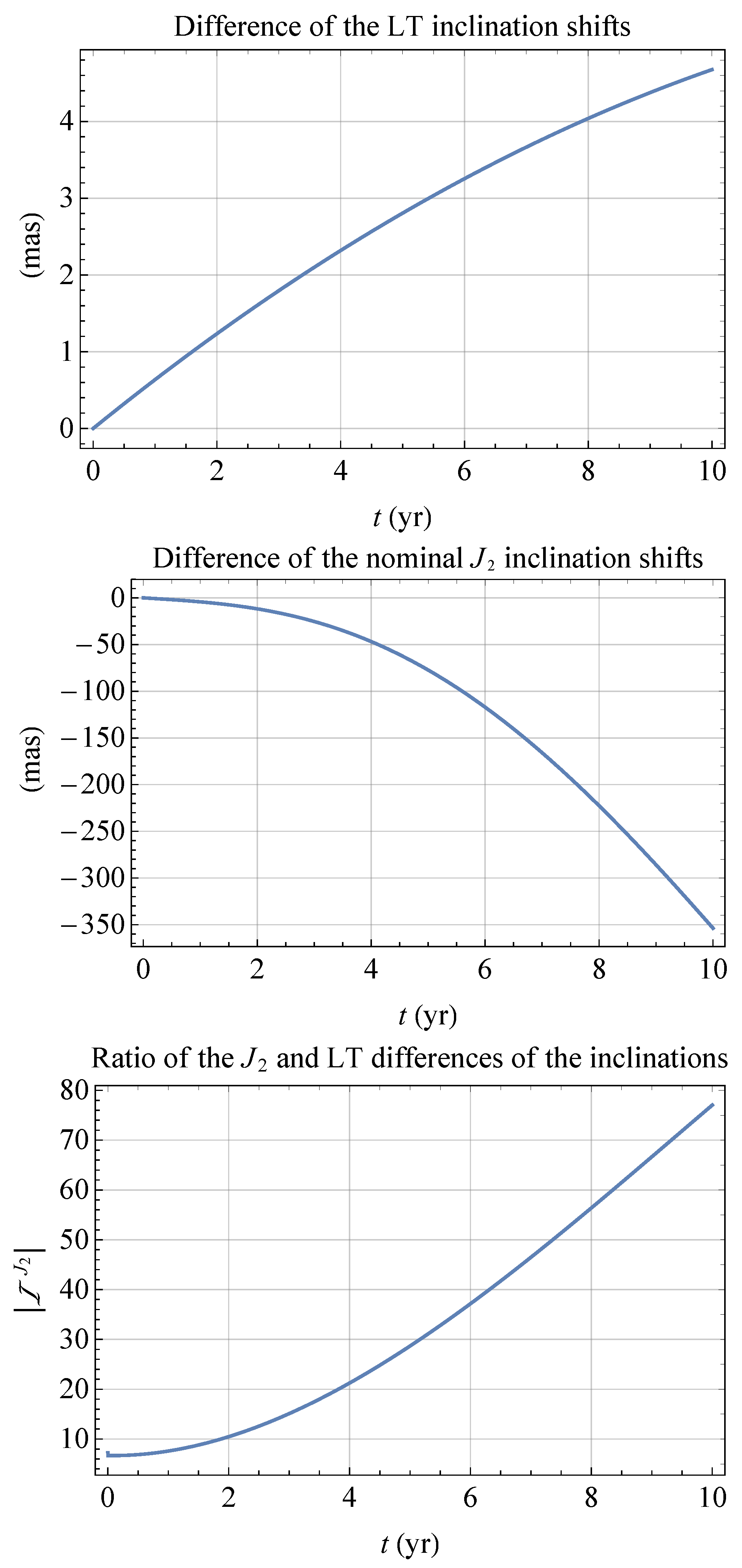
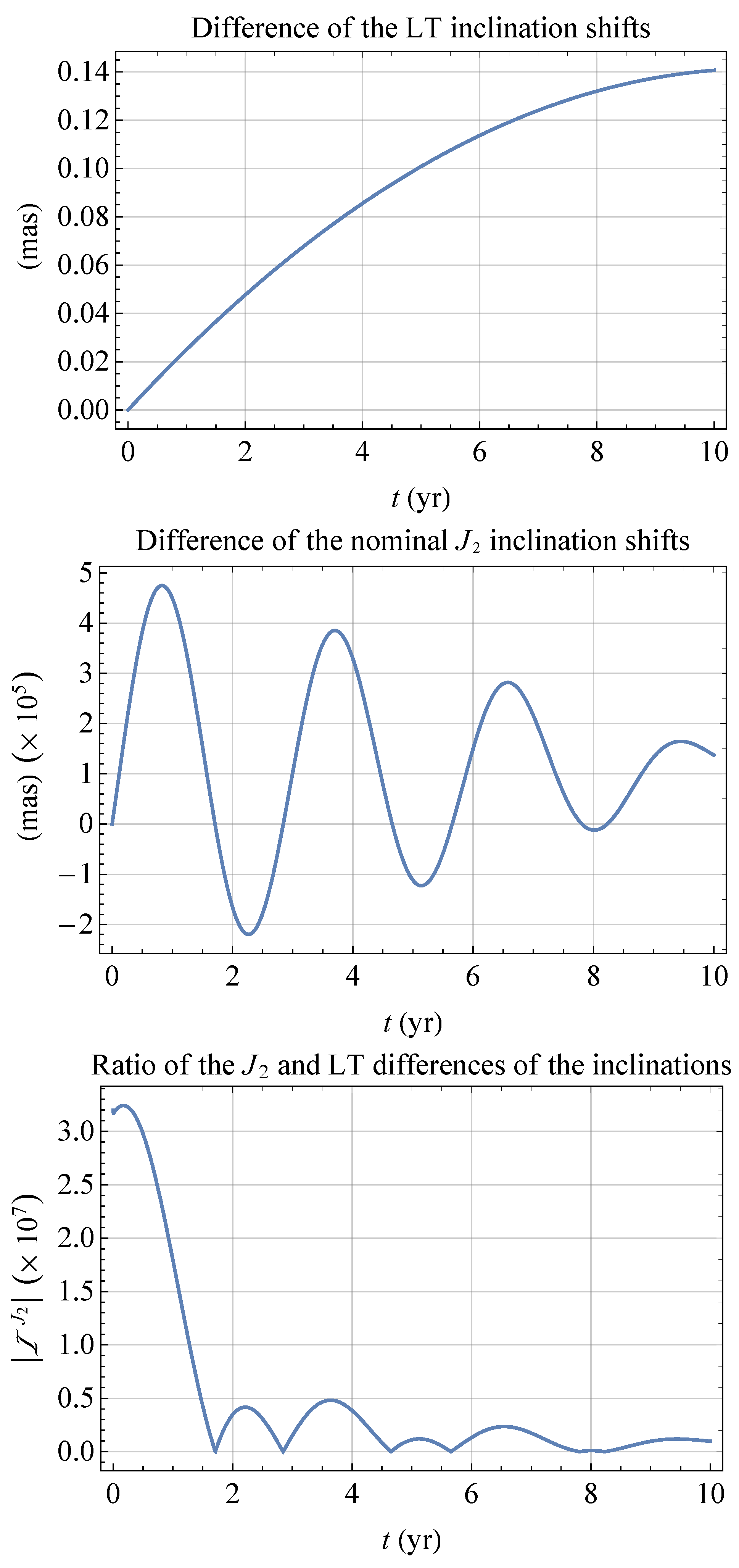
3.1. The Difference in the Inclinations

Figure 1 shows the plots of the differences in the nominal integrated shifts of the inclinations induced by the LT effect and the Earth’s oblateness, obtained for an orbital height of 2000 km for both spacecraft up to 4 km and almost-circular orbits whose eccentricities differed by $0.00376$. Equations (12) and (13) and Equations (21) and (22) were used for the initial values $I_0,{\Omega }_0$ of the inclinations and the nodes up to offsets of 10 mas in $I_0$ and 10 arcseconds in ${\Omega }_0$. Furthermore, the plot of the absolute value of

$${\mathcal{I}}^{J_2}\left(t\right):={\displaystyle \frac{\Delta I_{\mathrm{A}}^{J_2}\left(t\right)-\Delta I_{\mathrm{B}}^{J_2}\left(t\right)}{\Delta I_{\mathrm{A}}^{\mathrm{LT}}\left(t\right)-\Delta I_{\mathrm{B}}^{\mathrm{LT}}\left(t\right)}}$$

(24)

is also depicted. The ratio ${\mathcal{I}}^{J_2}$ is a measure of the nominal systematic bias induced by the Earth’s quadrupole mass moment on the expected LT signal; the larger it is, the greater the indirect impact of the errors of the various parameters ($G,J_2,R,\mathsf{\mu },J,a_{\mathrm{A},\mathrm{B}},e_{\mathrm{A},\mathrm{B}},I_{\mathrm{A},\mathrm{B}},{\Omega }_{\mathrm{A},\mathrm{B}},\dots$) entering it.

It turns out that the expected LT signal is at the mas level. However, the $J_2$ one is just up to about 80 times larger. Such a feature is important since it allows the mismodeling in Equation (24) induced by the several sources of errors affecting it to be made negligible. By varying the offsets in the orbital elements, it can be found that differences in the values of the semimajor axes and the eccentricities as large as those of the existing LAGEOS and LARES 2 [49] are well tolerated. Discrepancies in the initial values of the nodes from their ideal values of Equations (13) and (22) up to $\delta {\Omega }_0\simeq 0.1°$ would not yield a dramatic increase of ${\mathcal{I}}^{J_2}$. As far as the inclinations are concerned, departures from the ideal values of Equation (12) and Equation (21) up to $\delta I\simeq 100\mathrm{mas}$ would not change the pattern of Figure 1.

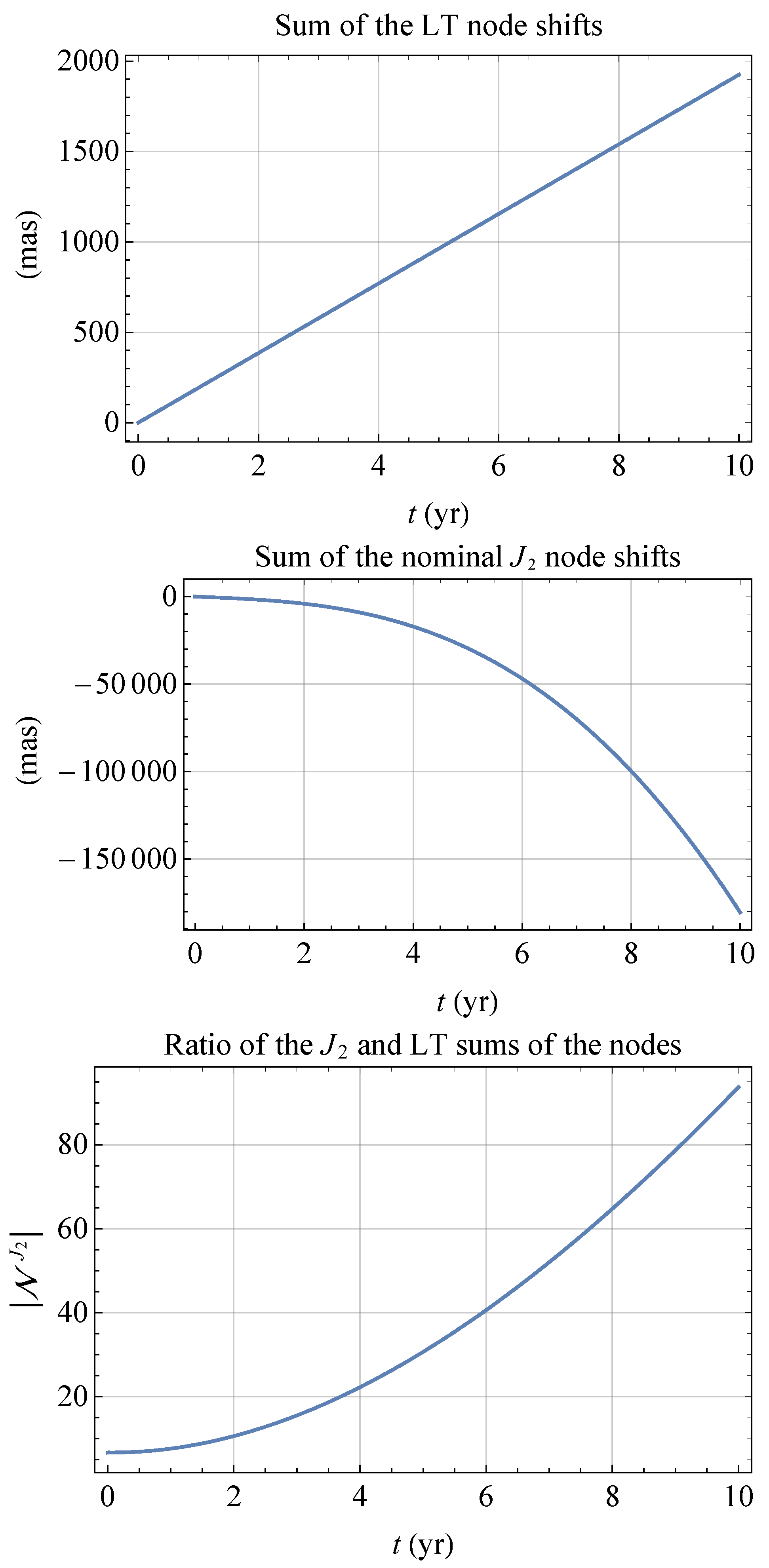
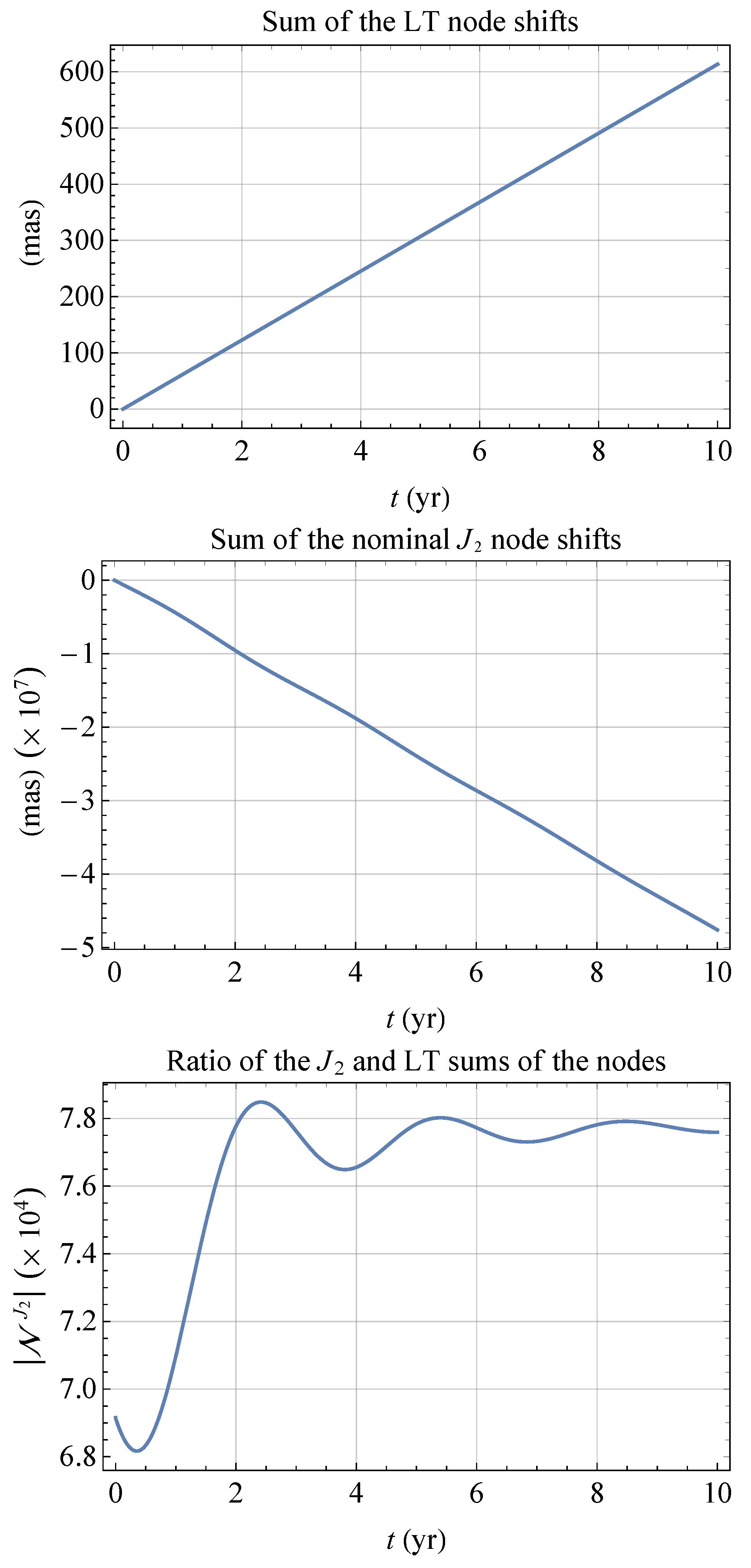
3.2. The Sum of the Nodes

By defining

$${\mathcal{N}}^{J_2}\left(t\right):={\displaystyle \frac{\Delta {\Omega }_{\mathrm{A}}^{J_2}\left(t\right)+\Delta {\Omega }_{\mathrm{B}}^{J_2}\left(t\right)}{\Delta {\Omega }_{\mathrm{A}}^{\mathrm{LT}}\left(t\right)+\Delta {\Omega }_{\mathrm{B}}^{\mathrm{LT}}\left(t\right)}},$$

(25)

it is possible to also repeat the previous analysis for the sum of the nodes of POLARES. The results are shown in Figure 2.

The combined LT signature reaches the arcsec level over 10 years, while the nominal bias due to $J_2$ is up to $\simeq 90$ times larger than the former over the same time span.

4. The LAGEOS–LARES 2 Case

Recently, Ciufolini and coworkers [56] claimed that LAGEOS and LARES 2 will allow them to perform a test of the LT effect accurate to $\simeq 0.2\%$ by monitoring the sum of their nodes, in accordance with the earlier proposal put forth by Ciufolini in [48].

In fact, all of the analyses by Ciufolini and coworkers over the years have always been based on Equations (9)–(11), which were not satisfied since the very epoch of the LARES 2 launch occurred about 22 years after J2000.0. On the other hand, even if Equations (10) and (11) could be applied to the LAGEOS–LARES 2 experiment, the present author showed in [50] that the ambitious goal by Ciufolini and coworkers [56] could not be met because of the consequences of the imperfect cancellation of the summed $J_2$-driven node precessions. By repeating the same analysis as in Section 3, one obtains Figure 3 and Figure 4, which clearly exemplify how it is not possible to achieve the accuracy goal stated in [56], not even when looking at the difference of the inclinations.

5. Summary and Conclusions

It has been shown that, for a general orientation of the primary’s spin axis with respect to the inertial reference frame adopted, the Lense–Thirring rates of change of the orbital inclinations of two satellites moving along ideally identical orbits in opposite directions are equal and opposite, while those induced by the primary’s oblateness have the same sign. However, the opposite happens for the nodes: the relativistic rates are the same, while the classical ones differ by a minus sign. Thus, the difference of the inclinations and the sum of the nodes of two counter-revolving spacecraft allow, in principle, for the aliasing Newtonian shifts to be cancelled out due to the quadrupole mass moment of the central body and for the gravitomagnetic ones to be enhanced.

The earlier proposal by Van Patten and Everitt—here branded POLARES—of using a pair of drag-free spacecrafts moving in opposite directions along identical circular orbits passing through the Earth’s poles is reexamined in view of the aforementioned results. Indeed, they would be applicable to a hypothesized new mission since at the time of its launch (still to come), the terrestrial spin axis would be displaced with respect to its orientation at the epoch J2000.0, which is generally assumed as the reference z axis of the geocentric inertial reference system usually adopted in actual satellites’ data reductions.

For an orbital altitude of, say, 2000 km, the combined relativistic inclination and node shifts of POLARES would amount to a few milliarcseconds and a couple of arcseconds, respectively, after 10 years from the launch. By assuming not-too-stringent orbital injection errors, the nominal ratios of the signatures due to the Earth’s first even zonal harmonic to the Lense–Thirring ones in both the difference of the inclinations and the sum of the nodes can be kept at a level sufficiently low to allow the indirect consequences on them of errors on the various physical and orbital parameters to be considered negligible.

This is not the case of the ongoing LAGEOS–LARES 2 experiment, both for the sum of the nodes and the difference of the inclinations, because of the imperfect cancellation of the classical orbital shifts for both the orbital elements.

Should the POLARES concept be implemented with passive, geodetic satellites of LAGEOS-type, a detailed investigation of several non-gravitational accelerations affecting them would be needed; this is outside the scope of the present paper.

References

1. Lense, J.; Thirring, H. Über den Einfluß der Eigenrotation der Zentralkörper auf die Bewegung der Planeten und Monde nach der Einsteinschen Gravitationstheorie. Phys. Z 1918, 19, 156–163. [Google Scholar]
2. Mashhoon, B.; Hehl, F.W.; Theiss, D.S. On the gravitational effects of rotating masses: The Thirring–Lense papers. Gen. Relativ. Gravit. 1984, 16, 711–750. [Google Scholar] [CrossRef]
3. Pfister, H. On the history of the so–called Lense–Thirring effect. Gen. Relativ. Gravit. 2007, 39, 1735–1748. [Google Scholar] [CrossRef]
4. Pfister, H. The History of the So–Called Lense–Thirring Effect. In the Eleventh Marcel Grossmann Meeting on Recent Developments in Theoretical and Experimental General Relativity, Gravitation and Relativistic Field Theories; Kleinert, H., Jantzen, R.T., Ruffini, R., Eds.; World Scientific: Singapore, 2008; pp. 2456–2458. [Google Scholar] [CrossRef]
5. Pfister, H. Gravitomagnetism: From Einstein’s 1912 Paper to the Satellites LAGEOS and Gravity Probe B. In Relativity and Gravitation; Bičák, J., Ledvinka, T., Eds.; Springer Proceedings in Physics; Springer: Cham, Switzerland, 2014; Volume 157, pp. 191–197. [Google Scholar] [CrossRef]
6. Cohen, S.C.; Smith, D.E. LAGEOS Scientific results: Introduction. J. Geophys. Res. 1985, 90, 9217–9220. [Google Scholar] [CrossRef]
7. Bardeen, J.M.; Petterson, J.A. The Lense–Thirring Effect and Accretion Disks around Kerr Black Holes. Astrophys. J. Lett. 1975, 195, L65. [Google Scholar] [CrossRef]
8. Rees, M.J. Relativistic jets and beams in radio galaxies. Nature 1978, 275, 516–517. [Google Scholar] [CrossRef]
9. Rees, M.J. Black Hole Models for Active Galactic Nuclei. Annu. Rev. Astron. Astr. 1984, 22, 471–506. [Google Scholar] [CrossRef]
10. Stone, N.; Loeb, A. Observing Lense-Thirring Precession in Tidal Disruption Flares. Phys. Rev. Lett. 2012, 108, 061302. [Google Scholar] [CrossRef]
11. Franchini, A.; Lodato, G.; Facchini, S. Lense–Thirring precession around supermassive black holes during tidal disruption events. Mon. Not. Roy. Astron. Soc. 2016, 455, 1946–1956. [Google Scholar] [CrossRef]
12. Pasham, D.R.; Zajaček, M.; Nixon, C.J.; Coughlin, E.R.; Śniegowska, M.; Janiuk, A.; Czerny, B.; Wevers, T.; Guolo, M.; Ajay, Y.; et al. Lense-Thirring precession after a supermassive black hole disrupts a star. Nature 2024, 630, 325–328. [Google Scholar] [CrossRef]
13. Stella, L.; Vietri, M. Lense–Thirring Precession and Quasi–periodic Oscillations in Low-Mass X-Ray Binaries. Astrophys. J. Lett. 1998, 492, L59–L62. [Google Scholar] [CrossRef]
14. Stella, L.; Possenti, A. Lense–Thirring Precession in the Astrophysical Context. Space Sci. Rev. 2009, 148, 105–121. [Google Scholar] [CrossRef]
15. Braginsky, V.B.; Caves, C.M.; Thorne, K.S. Laboratory experiments to test relativistic gravity. Phys. Rev. D 1977, 15, 2047–2068. [Google Scholar] [CrossRef]
16. Dymnikova, I.G. REVIEWS OF TOPICAL PROBLEMS: Motion of particles and photons in the gravitational field of a rotating body (In memory of Vladimir Afanas’evich Ruban). Sov. Phys. Usp. 1986, 29, 215–237. [Google Scholar] [CrossRef]
17. Tartaglia, A. Angular–momentum effects in weak gravitational fields. Europhys. Lett. 2002, 60, 167–173. [Google Scholar] [CrossRef]
18. Ruggiero, M.L.; Tartaglia, A. Gravitomagnetic effects. Nuovo Cim. B 2002, 117, 743. [Google Scholar] [CrossRef]
19. Schäfer, G. Gravitomagnetic Effects. Gen. Relativ. Gravit. 2004, 36, 2223–2235. [Google Scholar] [CrossRef]
20. Schäfer, G. Gravitomagnetism in Physics and Astrophysics. Space Sci. Rev. 2009, 148, 37–52. [Google Scholar] [CrossRef]
21. Pugh, G.E. (Ed.) Proposal for a Satellite Test of the Coriolis Prediction of General Relativity. In Nonlinear Gravitodynamics: The Lense-Thirring Effect; Research memorandum; Weapons Systems Evaluation Group, The Pentagon: Washington, DC, USA, 1959; Reprinted in Ruffini, R.J.; Sigismondi, C. (Eds.) Nonlinear Gravitodynamics: The Lense-Thirring Effect; World Scientific: Singapore, 2003; pp. 414–426. [Google Scholar]
22. Schiff, L. Possible new experimental test of general relativity theory. Phys. Rev. Lett. 1960, 4, 215–217. [Google Scholar] [CrossRef]
23. Everitt, C.W.F.; Debra, D.B.; Parkinson, B.W.; Turneaure, J.P.; Conklin, J.W.; Heifetz, M.I.; Keiser, G.M.; Silbergleit, A.S.; Holmes, T.; Kolodziejczak, J.; et al. Gravity Probe B: Final Results of a Space Experiment to Test General Relativity. Phys. Rev. Lett. 2011, 106, 221101. [Google Scholar] [CrossRef]
24. Everitt, C.W.F.; Muhlfelder, B.; Debra, D.B.; Parkinson, B.W.; Turneaure, J.P.; Silbergleit, A.S.; Acworth, E.B.; Adams, M.; Adler, R.; Bencze, W.J.; et al. The Gravity Probe B test of general relativity. Class. Quantum Gravit. 2015, 32, 224001. [Google Scholar] [CrossRef]
25. Everitt, C.W.F. The Gyroscope experiment—I: General description and analysis of gyroscope performance. In Proceedings of the International School of Physics “Enrico Fermi”. Course LVI. Experimental Gravitation; Bertotti, B., Ed.; Academic Press: Cambridge, MA, USA, 1974; pp. 331–360. [Google Scholar]
26. Everitt, C.W.F.; Buchman, S.; Debra, D.B.; Keiser, G.M.; Lockhart, J.M.; Muhlfelder, B.; Parkinson, B.W.; Turneaure, J.P.; Gravity Probe B team. Gravity Probe B: Countdown to Launch. In Gyros, Clocks, Interferometers…: Testing Relativistic Gravity in Space; Lämmerzahl, C., Everitt, C.W.F., Hehl, F.W., Eds.; Lecture Notes in Physics; Springer: Berlin/Heidelberg, Germany, 2001; Volume 562, pp. 52–82. [Google Scholar] [CrossRef]
27. Park, R.S.; Folkner, W.M.; Konopliv, A.S. Estimation of Solar Angular Momentum from Lense–Thirring Precession of Mercury. Iau Gen. Assem. 2015, 22, 2227771. [Google Scholar]
28. Pavlov, D.; Dolgakov, I. General relativity tests by the dynamics of the Solar system. In Journées 2023 “Systèmes de Rférénce Spatio-Temporels"; Bizouard, C., Fienga, A., Paganelli, F., Eds.; Observatoire de la Côte d’Azur, 2024; pp. 156–160. [Google Scholar]
29. Pavlov, D.; Dolgakov, I. Studying the Properties of Spacetime with an Improved Dynamical Model of the Inner Solar System. Universe 2024, 10, 413. [Google Scholar] [CrossRef]
30. Bolton, S.J.; Lunine, J.; Stevenson, D.; Connerney, J.E.P.; Levin, S.; Owen, T.C.; Bagenal, F.; Gautier, D.; Ingersoll, A.P.; Orton, G.S.; et al. The Juno Mission. Space Sci. Rev. 2017, 213, 5–37. [Google Scholar] [CrossRef]
31. Finocchiaro, S.; Iess, L.; Folkner, W.M.; Asmar, S. The Determination of Jupiter’s Angular Momentum from the Lense-Thirring Precession of the Juno Spacecraft. In Proceedings of the AGU Fall Meeting Abstracts, San Francisco, CA, USA, 5–9 December 2011; Volume 2011, p. P41B-1620. [Google Scholar]
32. Durante, D.; Cappuccio, P.; di Stefano, I.; Zannoni, M.; Casajus, L.G.; Lari, G.; Falletta, M.; Buccino, D.R.; Iess, L.; Park, R.S.; et al. Testing General Relativity with Juno at Jupiter. Astrophys. J. 2024, 971, 145. [Google Scholar] [CrossRef]
33. Ciufolini, I.; Lucchesi, D.M.; Vespe, F.; Mandiello, A. Measurement of dragging of inertial frames and gravitomagnetic field using laser–ranged satellites. Nuovo Cim. A 1996, 109A, 575–590. [Google Scholar] [CrossRef]
34. Pearlman, M.; Arnold, D.; Davis, M.; Barlier, F.; Biancale, R.; Vasiliev, V.; Ciufolini, I.; Paolozzi, A.; Pavlis, E.C.; Sośnica, K.; et al. Laser geodetic satellites: A high-accuracy scientific tool. J. Geod. 2019, 93, 2181–2194. [Google Scholar] [CrossRef]
35. Coulot, D.; Deleflie, F.; Bonnefond, P.; Exertier, P.; Laurain, O.; de Saint-Jean, B. Satellite Laser Ranging. In Encyclopedia of Solid Earth Geophysics; Gupta, H.K., Ed.; Encyclopedia of Earth Sciences Series; Springer: Berlin/Heidelberg, Germany, 2011; pp. 1049–1055. [Google Scholar] [CrossRef]
36. Iorio, L.; Lichtenegger, H.I.M.; Ruggiero, M.L.; Corda, C. Phenomenology of the Lense–Thirring effect in the solar system. Astrophys. Space Sci. 2011, 331, 351–395. [Google Scholar] [CrossRef]
37. Ciufolini, I.; Paolozzi, A.; Koenig, R.; Pavlis, E.C.; Ries, J.; Matzner, R.; Gurzadyan, V.; Penrose, R.; Sindoni, G.; Paris, C. Fundamental Physics and General Relativity with the LARES and LAGEOS satellites. Nucl. Phys. B Proc. Suppl. 2013, 243, 180–193. [Google Scholar] [CrossRef]
38. Renzetti, G. History of the attempts to measure orbital frame–dragging with artificial satellites. Centr. Eur. J. Phys. 2013, 11, 531–544. [Google Scholar] [CrossRef]
39. Lucchesi, D.M.; Anselmo, L.; Bassan, M.; Magnafico, C.; Pardini, C.; Peron, R.; Pucacco, G.; Visco, M. General Relativity Measurements in the Field of Earth with Laser–Ranged Satellites: State of the Art and Perspectives. Universe 2019, 5, 141. [Google Scholar] [CrossRef]
40. Lucchesi, D.M.; Visco, M.; Peron, R.; Bassan, M.; Pucacco, G.; Pardini, C.; Anselmo, L.; Magnafico, C. A 1% Measurement of the Gravitomagnetic Field of the Earth with Laser–Tracked Satellites. Universe 2020, 6, 139. [Google Scholar] [CrossRef]
41. Milani, A.; Nobili, A.; Farinella, P. Non–Gravitational Perturbations and Satellite Geodesy; Adam Hilge: London, UK, 1987. [Google Scholar]
42. Lucchesi, D.M. Reassessment of the error modelling of non–gravitational perturbations on LAGEOS II and their impact in the Lense–Thirring determination. Part I. Planet. Space Sci. 2001, 49, 447–463. [Google Scholar] [CrossRef]
43. Lucchesi, D.M. Reassessment of the error modelling of non–gravitational perturbations on LAGEOS II and their impact in the Lense–Thirring derivation–Part II. Planet. Space Sci. 2002, 50, 1067–1100. [Google Scholar] [CrossRef]
44. Lucchesi, D.M. LAGEOS Satellites Germanium Cube–Corner-Retroreflectors and the Asymmetric Reflectivity Effect. Celest. Mech. Dyn. Astr. 2004, 88, 269–291. [Google Scholar] [CrossRef]
45. Lucchesi, D.M.; Ciufolini, I.; Andrés, J.I.; Pavlis, E.C.; Peron, R.; Noomen, R.; Currie, D.G. LAGEOS II perigee rate and eccentricity vector excitations residuals and the Yarkovsky–Schach effect. Planet. Space Sci. 2004, 52, 699–710. [Google Scholar] [CrossRef]
46. Van Patten, R.A.; Everitt, C.W.F. A Possible Experiment with Two Counter-Orbiting Drag-Free Satellites to Obtain a New Test of Einstein’s General Theory of Relativity and Improved Measurements in Geodesy. Celest. Mech. Dyn. Astr. 1976, 13, 429–447. [Google Scholar] [CrossRef]
47. Van Patten, R.A.; Everitt, C.W.F. Possible experiment with two counter-orbiting drag-free satellites to obtain a new test of Einstein’s general theory of relativity and improved measurements in geodesy. Phys. Rev. Lett. 1976, 36, 629–632. [Google Scholar] [CrossRef]
48. Ciufolini, I. Measurement of the Lense-Thirring drag on high-altitude, laser-ranged artificial satellites. Phys. Rev. Lett. 1986, 56, 278–281. [Google Scholar] [CrossRef]
49. Ciufolini, I.; Paolozzi, A.; Pavlis, E.C.; Ries, J.C.; Matzner, R.; Paris, C.; Ortore, E.; Gurzadyan, V.; Penrose, R. The LARES 2 satellite, general relativity and fundamental physics. Eur. Phys. J. C 2023, 83, 87. [Google Scholar] [CrossRef]
50. Iorio, L. Limitations in Testing the Lense–Thirring Effect with LAGEOS and the Newly Launched Geodetic Satellite LARES 2. Universe 2023, 9, 211. [Google Scholar] [CrossRef]
51. Iorio, L. A new proposal for measuring the Lense-Thirring effect with a pair of supplementary satellites in the gravitational field of the Earth. Phys. Lett. A 2003, 308, 81–84. [Google Scholar] [CrossRef]
52. Souchay, J.; Capitaine, N. Precession and Nutation of the Earth. In Tides in Astronomy and Astrophysics; Souchay, J., Mathis, S., Tokieda, T., Eds.; Lecture Notes in Physics; Springer: Berlin/Heidelberg, Germany, 2013; Volume 861, pp. 115–166. [Google Scholar] [CrossRef]
53. Petit, G.; Luzum, B. (Eds.) IERS Conventions (2010); IERS Technical Note; Verlag des Bundesamts für Kartographie und Geodäsie: Frankfurt am Main, Germany, 2010; Volume 36. [Google Scholar]
54. Capitaine, N.; Wallace, P.T. High precision methods for locating the celestial intermediate pole and origin. Astron. Astrophys. 2006, 450, 855–872. [Google Scholar] [CrossRef]
55. Montenbruck, O.; Gill, E. Satellite Orbits; Spinger: Berlin/Heidelberg, Germany, 2000. [Google Scholar] [CrossRef]
56. Ciufolini, I.; Paris, C.; Pavlis, E.C.; Ries, J.C.; Matzner, R.; Deka, D.; Ortore, E.; Kuzmicz-Cieslak, M.; Gurzadyan, V.; Penrose, R.; et al. On the high accuracy to test dragging of inertial frames with the LARES 2 space experiment. Eur. Phys. J. C 2024, 84, 998. [Google Scholar] [CrossRef]
Figure 1. Differences in the nominal LT (upper panel) and J 2 (middle panel) shifts of the inclinations, in mas, of a pair of counter-orbiting satellites numerically integrated over 10 years. The temporal variations of both k ^ ([55] pp. 176–177) and J 2 , modeled according to ITSG-Grace2018, were included as well. An initial epoch 35 years after J2000.0 was assumed. An orbital height of 2000 km was adopted for both satellites up to an offset of 10 km. The initial values of the inclinations differ from Equations (12) and (13) and Equations (21) and (22) by 10 mas. The lower panel shows the plot of the absolute value of Equation (24).
Universe 10 00447 g001
Figure 2. Sums of the nominal LT (upper panel) and J 2 (middle panel) shifts of the nodes, in mas, of a pair of counter-orbiting satellites numerically integrated over 10 years. The temporal variations of both k ^ ([55] pp. 176–177) and J 2 , modeled according to ITSG-Grace2018, were included as well. An initial epoch 35 years after J2000.0 was assumed. An orbital height of 2000 km was adopted for both satellites up to an offset of 10 km. The initial values of the inclinations differ from Equations (12) and (13) and Equations (21) and (22) by 10 mas. The lower panel shows the plot of the absolute value of Equation (25).
Universe 10 00447 g002
Figure 3. Differences in the nominal LT (upper panel) and J 2 (middle panel) shifts of the inclinations, in mas, of LAGEOS and LARES 2 numerically integrated over 10 years. The temporal variations of both k ^ ([55] pp. 176–177) and J 2 , modeled according to ITSG-Grace2018, were included as well. The launch date of LARES 2 was assumed as the initial epoch. The initial values of the satellites’ semimajor axis, eccentricity and inclination were retrieved from ([49] Table 1), while those of the nodes were calculated with the WEB resource https://www.n2yo.com/ (accessed on 1 November 2024). The lower panel shows the plot of the absolute value of Equation (24).
Universe 10 00447 g003
Figure 4. Sums of the nominal LT (upper panel) and J 2 (middle panel) shifts of the nodes, in mas, of LAGEOS and LARES 2 numerically integrated over 10 years. The temporal variations of both k ^ ([55] pp. 176–177) and J 2 , modeled according to ITSG-Grace2018, were included as well. The launch date of LARES 2 was assumed as the initial epoch. The initial values of the satellites’ semimajor axis, eccentricity and inclination were retrieved from ([49] Table 1), while those of the nodes were calculated with the WEB resource https://www.n2yo.com/ (accessed on 1 November 2024). The lower panel shows the plot of the absolute value of Equation (25).
Universe 10 00447 g004
Disclaimer/Publisher’s Note: The statements, opinions and data contained in all publications are solely those of the individual author(s) and contributor(s) and not of MDPI and/or the editor(s). MDPI and/or the editor(s) disclaim responsibility for any injury to people or property resulting from any ideas, methods, instructions or products referred to in the content.