CESE Schemes for Solar Wind Plasma MHD Dynamics

Abstract

Magnetohydrodynamic (MHD) numerical simulation has emerged as a pivotal tool in space physics research, witnessing significant advancements. This methodology offers invaluable insights into diverse space physical phenomena based on solving the fundamental MHD equations. Various numerical methods are utilized to approximate the MHD equations. Among these, the space–time conservation element and solution element (CESE) method stands out as an effective computational approach. Unlike traditional numerical schemes, the CESE method significantly enhances accuracy, even at the same base point. The concurrent discretization of space and time for conserved variables inherently achieves higher-order accuracy in both dimensions, without the need for intricate higher-order time discretization processes, which are often challenging in other methods. Additionally, this scheme can be readily extended to multidimensional cases, without relying on operator splitting or direction alternation. This paper primarily delves into the remarkable progress of CESE MHD models and their applications in studying solar wind, solar eruption activities, and the Earth’s magnetosphere. We aim to illuminate potential avenues for future solar–interplanetary CESE MHD models and their applications. Furthermore, we hope that the discussions presented in this review will spark new research endeavors in this dynamic field.

1. Introduction

MHD numerical simulation plays a crucial role in space physics research and has experienced rapid development. It offers a valuable tool for investigating various space physics phenomena by solving the governing equations of MHD, enabling the tracing of event evolution and the exploration of underlying physical mechanisms. By quantifying the content described by theoretical physical models and providing spatial and temporal distributions of physical quantities, MHD simulation allows for the tracing and prediction of the development and changes in these quantities. This makes it particularly suitable for studying the evolution of space physical phenomena in the Sun–Earth space domain. MHD numerical simulation acts as a bridge between satellite observations and theoretical analysis. Satellite observations are utilized to define the internal boundary conditions for MHD numerical simulation, and various numerical methods (such as the finite difference, finite volume, finite element, and time–space conservation element and solution element methods) are employed to approximate the control equations of MHD, facilitating the tracing of the temporal and spatial evolution of each variable. CESE is an effective computational method of conservation equations. It was firstly proposed by Chang [1] from the NASA Lewis Research Center in 1995. This method is fundamentally different from the traditional method: The cornerstone principle of the CESE method revolves around the integrated treatment of space and time as a single entity in the computation of flux balance, distinguishing it fundamentally from conventional numerical methodologies. Furthermore, a second distinctive feature lies in the CESE approach, wherein spatial derivatives are regarded as variables to be solved, marking a departure from other numerical methods in this regard. Feng [2] pointed out that the physical parameters are defined to have smooth profiles inside an SE, while between SEs or in CEs, they may be discontinuous. This is the typical reason why the CESE method can capture sharp discontinuity within a few grid points. It can greatly improve the accuracy of the scheme under the same base point. The simultaneous discretization of space and time for each conserved variable can naturally reach a higher order in time and space at the same time, and there is no need for a separate complicated processing of the higher-order discretization of time, which is difficult to achieve in other methods. Another advantage of the CESE method is that the structure is relatively simple: in addition to the simple Taylor expansion, no other numerical methods are used, especially the need to use other feature analysis numerical methods (such as the Riemann solver) to capture shock waves and suppress oscillations. Moreover, the scheme can be directly generalized to multidimensional cases without operator splitting or direction alternation. In short, the CESE method has clear physical meaning, high resolution, simple format structure, and a very broad application prospect. In a series of papers [1,3,4,5,6,7], Chang and his collaborators have achieved notable success in formulating and extensively applying the CESE method to the realm of hydrodynamics (HD). This innovative technique has proven to be highly effective in solving both linear and nonlinear convection–diffusion equations across various spatial dimensions, spanning from one to three dimensions. The CESE method has garnered widespread adoption in investigating diverse flow phenomena, including those involving moving and stationary shocks, acoustic waves, intricate vertical flows, detonations, and complex interactions among shock waves, acoustic phenomena, and vortices, as well as dam-break flows. For a comprehensive overview of the evolution and advancements of the CESE method, readers are encouraged to refer to the seminal work by Wang [8]. Feng et al. [9] and Hu and Feng [10] firstly extended the original second-order CESE method to 2.5-dimensional resistive MHD equations in Cartesian coordinates and applied to model the magnetic reconnection study. Further, it is widely used in MHD numerical simulations and well applied to study the evolution and development of the solar corona and heliosphere. This method was well-tested as a robust and versatile scheme for solving a wide range of MHD problems from data-driven simulation of active region evolutions [11] to the global solar wind modeling [12] as well as the global magnetosphere models [8]. This method has undergone rigorous testing, proving itself to be a robust and adaptable framework for tackling a diverse array of MHD challenges, ranging from data-driven simulations of active region evolution, as demonstrated in [11], to the comprehensive modeling of the global solar wind, as exemplified in [12], encompassing even the intricate global magnetosphere models, as outlined in [8]. In this review, we mainly focus on describing the current significant progress of CESE MHD models and their applications in the study of the solar wind, solar eruption activities, and the Earth’s magnetosphere response to the solar wind. We try to shed light on future avenues of solar–interplanetary CESE MHD models and their applications. We also hope that the discussions in this review will be of some help to inspire new research outcomes in this field.

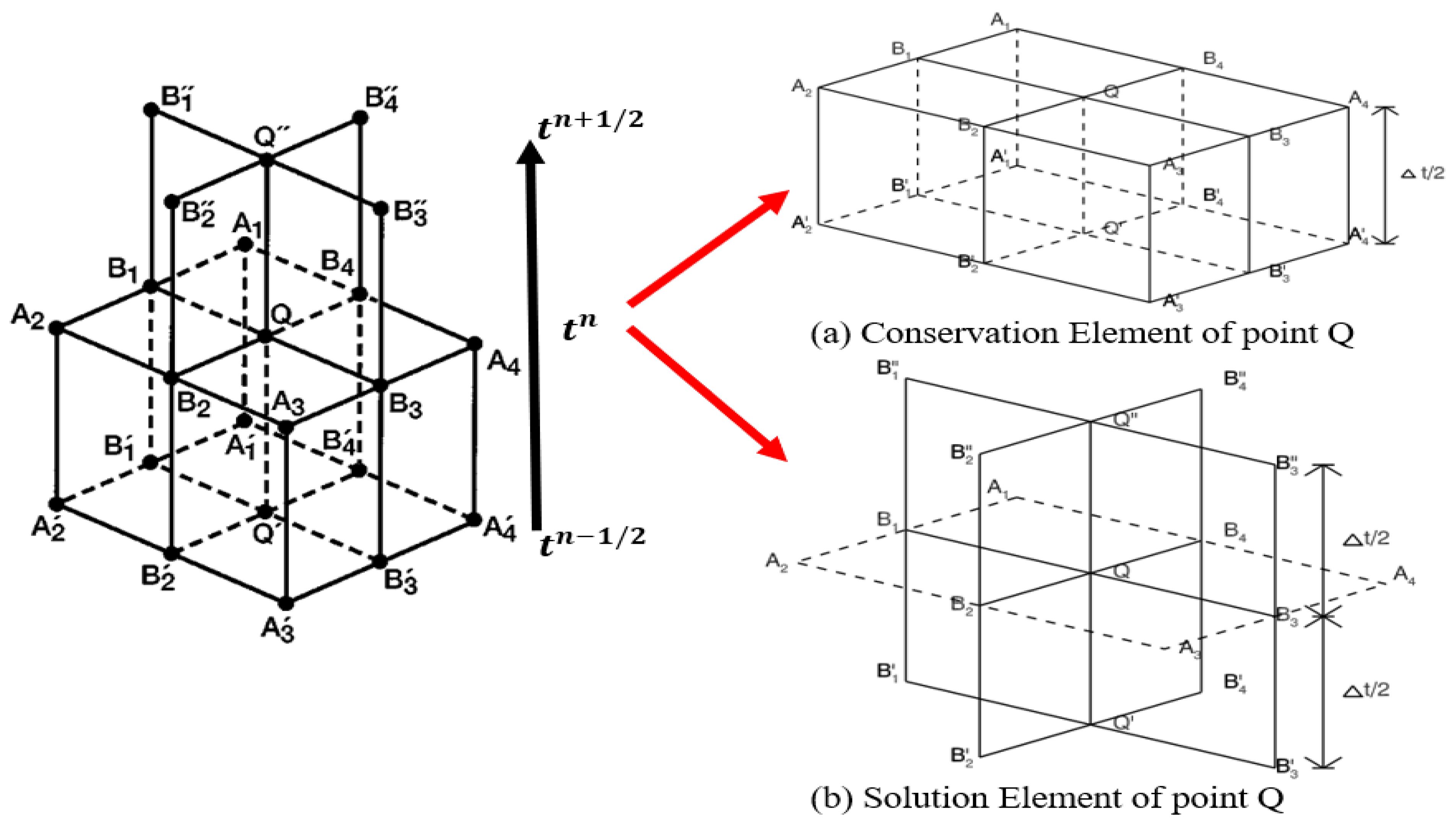
2. Brief Introduction to CESE Method

The CESE method is a cutting-edge numerical technique for solving conservation equations. It represents a paradigm shift in the traditional approaches to conservation modeling by treating time and space as equal partners. This method utilizes conservation-type integral equations and defines conservation elements and solution elements to ensure that the local and global conservation laws are strictly adhered to. A key advantage of the CESE method is its ability to simultaneously determine the physical quantities and their spatial derivatives at grid points. This approach significantly reduces numerical errors compared with traditional difference schemes, resulting in higher computational accuracy. Moreover, the CESE method is particularly suited for capturing discontinuous flow fields, exhibiting high resolution and satisfactory results. The simplicity of the CESE method is another notable feature. It relies primarily on Taylor expansions and does not require complex numerical approximation techniques or characteristic decomposition methods. This makes it easier to implement and extend to multidimensional problems without resorting to operator splitting or directional alternating techniques. In summary, the CESE method is a powerful tool for simulating complex conservation phenomena. Its unique approach of unifying time and space, along with its high accuracy, resolution, and simplicity, makes it an attractive choice for a wide range of applications in fluid dynamics, magnetohydrodynamics, and other fields. The reader is presupposed to possess a foundational understanding of the fundamental concepts of CESE numerical methods pertaining to partial differential equations in a general context. For those seeking to bolster their essential background in this area, we encourage the consultation of pertinent references (e.g., [2,13,14]), which provide a comprehensive overview of the underlying principles and applications of these methods.

Let us take solving two-dimensional (2D) nonlinear equations as an example to introduce the implementation process of the CESE method. The 2D nonlinear equations in conservative form are as follows:

$${\displaystyle \frac{\partial U}{\partial t}}+{\displaystyle \frac{\partial F\left(U\right)}{\partial x}}+{\displaystyle \frac{\partial G\left(U\right)}{\partial y}}=0$$

(1)

where $U=(u_1,u_2,\cdots ,u_m)$ is the state vector of the conservative variables. $F\left(U\right)=(f_1,f_2,\cdots ,f_m)$ and $G\left(U\right)=(g_1,g_2,\cdots ,g_m)$ denote the flux vector in the x- and y-directions, respectively. The most significant feature of the CESE scheme is to unify time and space into a conservation relation. In the generalized 3D Euclidean space $E_{2+1}(x,y,t)$, which combines the spatial coordinates with time, Equation (1) can be rewritten as

$$\nabla ·{\mathbf{h}}_m=0,$$

(2)

where ${\mathbf{h}}_m=(u_m,f_m,g_m)$ is the space–time flux vector.

By applying Gauss’s divergence theorem to Equation (2) in the 3D space–time domain $E_{2+1}(x,y,t)$, one can obtain

$$\underset{S\left(V\right)}{\oint }{\mathbf{h}}_m·d\mathbf{s}=0,$$

(3)

where $S\left(V\right)$ is the boundary of any closed space–time region V in $E_{2+1}(x,y,t)$. ${\mathbf{h}}_m·d\mathbf{s}$ denotes the total space–time flux leaving the surface element $d\mathbf{s}$. $Q^{*}$ denotes the solution point, and its conservation elements (CEs) is represented by the hexahedron $A_1{B}_1{A}_2{B}_2{A}_3{B}_3{A}_4{B}_4{A}_1^{\prime }{B}_1{A}_2^{\prime }{B}_2^{\prime }{A}_3^{\prime }{B}_3^{\prime }{A}_4^{\prime }{B}_4^{\prime }$, as shown in Figure 1a. The SE of point Q is the union of the three plane segments $B_1{B}_3{B}_1{B}_3,$ $B_2{B}_4{B}_2{B}_4$, and $A_1{B}_1{A}_2{B}_2{A}_3{B}_3{A}_4{B}_4$, as shown in Figure 1b. In addition to the method shown in Figure 1, there are also various other ways to construct CEs and SEs, as long as all the constructed CEs can cover the entire space–time domain and that their SEs cover the boundaries of all the CEs but never overlap with each other. Because the conservation law, i.e., Equation (3), is suitable for an arbitrary closed space–time domain, generally, it is the best choice to build CEs that can facilitate the derivation of the discrete form of Equation (3). In SEs, since the values of variables and fluxes are continuous, the value at any point in an SE can be approximated from the value of known points through Taylor expansion, and the order of Taylor expansion determines the order of the scheme. After the integration over all the boundary surfaces of CEs, we obtain the updated variables $U_{updated}$ as follows:

$$U_{updated}={\displaystyle \frac{(I_{bottom}-I_{side}-I_{top}^{*})}{S}},$$

(4)

where $I_{bottom}$ and $I_{side}$ represent the space–time flux integration on the bottom and side surface of the CEs, respectively. $I_{top}^{*}$ is the higher-order part of flux integration on the top surface where the solution point is located, and S is the area of the top surface. The detailed derivation process of Equation (4) can be found in Yang et al. [15]. $I_{bottom}$, $I_{side}$, and $I_{top}^{*}$ are all functions of the conservative variables $u_m$, flux $f_m$, $g_m$, and their derivatives with respect to $x,y,$ and t. The derivatives of flux $f_m$ and $g_m$ can be obtained from the derivatives of conservative variables according to the chain rule, such as ${\displaystyle \frac{f_m}{\phi }}={\displaystyle \sum _i^m}{\displaystyle \frac{f_m}{u_i}}{\displaystyle \frac{u_i}{\phi }},\phi =x,y,t$. The derivatives with respect to t of conservative variables $u_{mt}$ can be obtained through the derivatives of flux $f_m$ and $g_m$ according to the conservation law expressed by Equation (3), namely, $u_{mt}=-f_{mx}-g_{my}$. Therefore, in the end, to update the conservative variables of Equation (4), one only needs to obtain the derivatives of conservative variables with respect to spatial coordinate variables for all orders. For example, for the 2D second-order scheme, one needs to update the values of $u_m,u_{mx},$ and $u_{my}$.

3. Development of CESE-MHD Models and Their Applications

Chang and his team have triumphantly devised the CESE method and have successfully implemented it across a broad spectrum of applications in hydrodynamics (HD), proficiently addressing both linear and nonlinear convection–diffusion equations and nonlinear convection–diffusion equations across various spatial dimensions, spanning from one to three dimensions. The CESE method has been used to study flows with moving and steady shock, acoustic waves, complex vertical flows, detonations, and intricate interactions among shock waves, acoustics, and vortices, as well as dam-break flows. Feng and his team popularized and applied it to the MHD and the simulation of the solar–terrestrial space environment in the past decade or so and made a series of achievements in the improvement and application of this method. The following is a summary of these achievements from three perspectives: CESE-MHD models and their applications in the study of the solar wind, solar eruption activities, and the Earth’s magnetosphere.

3.1. CESE-MHD Models Applied to Background Solar Wind

It is well known that the solar wind ambient is important in the study of coronal and interplanetary space. The numerical models of solar wind mainly include two types. (1) Empirically and numerically based models: This type of model considers different solar wind solution in the coronal and the heliospheric region separately. (2) Complete MHD numerical models: This type of model only utilizes single solar wind numerical solutions through the coronal and the heliospheric region. CORona-HELiosphere is a coupled suite of models for quantitatively modeling the solar corona and solar wind in 3D space, and it is developed by the Center for Integrated Space Weather Modeling (CISM) [17]. The Wang–Sheeley–Arge (WSA)/ENLIL [18] in the CISM is the most successful space weather model that belongs to the first style. The WSA model is employed to determine solar coronal parameters and to provide inner boundary conditions for heliospheric MHD models according to an empirical relationship. The magnetohydrodynamics around a sphere (MAS) [19,20] model in the CISM, Block-Adaptive-Tree-Solarwind-Roe-Upwind-Scheme (BATS-R-US) code in the SWMF (Space Weather Modeling Framework) [21], and the solar–interplanetary conservative element solution element MHD (SIP-CESE MHD) model in the SWIM (Space Weather Integrated Model) are the most commonly used models that belong to the second style. These are the most advanced three-dimensional (3D) time-dependent numerical simulation models of solar wind. Wu and Dryer [22] presented a comparative study of these three models. In this review, we mainly introduce the development of the SIP-CESE MHD model. Modeling the solar wind by using the CESE method is not a straightforward process, necessitating the reformulation of the grid mesh to ensure its suitability for accurate solar wind simulation. Feng et al. [23] and Hu et al. [24] devised the 3D Solar–Interplanetary space–time Conservation Element and Solution Element (SIP-CESE) MHD model, tailored for solar wind modeling on triangular prism grids within a spherical geometry. Firstly, 3D pentahedral cells are established, with each cell being a triangular prism composed of two triangular bases and three rectangular sides, on which to approximate the solar wind MHD solution. Figure 2a illustrates the intricate grid structure at the spherical inner boundary. Subsequently, the spherical surface is expanded at varying radial distances by introducing a radial variation formula, where $r\left(1\right)=1R_s,r\left(i\right)=r(i-1)+step\times r(i-1)withstep={\displaystyle \frac{\pi }{60}}$. This approach divides the 3D spatial computational domain into non-overlapping convex pentahedrons, where any two adjacent pentahedrons share a common surface. Each pentahedral cell comprises a triangular prism, structured by two triangular bases and three rectangular sides. Figure 2b showcases a segment of these pentahedrons and the methodology for constructing the 3D grid structure by extending the positions of the spherically arranged grids outward from the inner boundary. The SIP-CESE MHD model established on triangular prism grids has been applied in simulating the 2D coronal dynamical structure with multi-pole magnetic fields and the 3D coronal dynamical structure and for investigating the evolution of the large-scale coronal magnetic structure during solar cycle 23.

These examples show that the SIP-CESE MHD model possesses the ability to model the Sun–Earth environment. For solar wind research, the 3D SIP-CESE-MHD model [23,24,25,26,27] is the basic model. Later, enhanced with the incorporation of new numerical features, this model has undergone significant improvement. These new numerical features mainly include grid systems, the Courant Number Insensitive (CNIS) method [28,29], the multigrid projection method with magnetic field divergence cleaning procedure, the multi-time-stepping method [30,31], and volumetric heating [32,33]. For grid systems, Feng et al. [34] devised a composite mesh comprising six identical component meshes, strategically designed to overlap partially on their boundaries as they collectively cover a spherical surface. This innovative grid system adeptly circumvents issues of mesh convergence and singularities that typically plague pole regions. Furthermore, the grid system facilitates seamless parallelization not only along the ($\theta ,\varphi$) directions but also in the radial dimension, enhancing computational efficiency. To mitigate high numerical dissipation in regions characterized by small CFL numbers, the CNIS method was introduced, ensuring that the accuracy of the solution remains intact. The projection method is chosen to fix the magnetic field divergence error caused by the numerical scheme, since it does not depend on specific differences and can achieve a better result compared with other methods [35,36]. The approximate projection operator [37] with the full multigrid (F-cycle) method [38] described below is employed to solve the Poisson equation. The F-cycle iteration can maintain the $\nabla ·\mathrm{B}$ error at an acceptable level of ${10}^{-6}$, and it has a proper time–cost performance of about $40\%$ CPU time in the time step. In time integration, the multi-time-stepping method is used by dividing the solar–terrestrial space into six sub-domains. This method enhances the convergence stability and speeds up the calculation by easing CFL number disparity. For the acceleration of solar wind, volumetric heating source terms are considered by using a 3D distribution profile based on the expansion factor $f_s$ and the angular distance ${\theta }_b$. The heating intensity diminishes in regions where the magnetic field experiences over-radial expansion ($f_s>1.0$), whereas it intensifies at locations where the magnetic field undergoes under-radial expansion ($f_s<1.0$). Employing the angular distance parameter ${\theta }_b$ offers a precise means of differentiating between high-speed and low-speed solar winds. Specifically, high-speed solar winds originating from the center of coronal holes exhibit a substantial ${\theta }_b$, whereas low-speed winds emanating from the boundaries of these holes are characterized by a smaller ${\theta }_b$. After the above series of improvements, the SIP-CESE MHD model can realistically generate structured solar wind. In Figure 3 and Figure 4, there is overall strong concordance between the simulations and observations, with the simulation accurately replicating the observed high-speed wind segments exceeding >500 km s⁻¹, along with their intricate structural variations. The good agreement between numerical results and observations at 1 AU demonstrate the efficiency, accuracy, and ability to reasonably produce structured solar wind of the model. To solve the problem of the disparate temporal and spatial scales of multiple physical process in different domains, the SIP-CESE MHD model is embedded into a package, PARAMESH 3.3, which offers the scalable, massively parallel, block-based adaptive-mesh refinement (AMR) technique, which allows for the solution of such disparate spatial and temporal scales throughout the computational domain with even fewer cells but can generate the necessary resolution. It is also called the AMR-CESE-MHD model. Two AMR realization strategies are implemented: one is to employ a solution-adaptive technique directly for the CESE solver in the six-component grid system extracted from Feng et al. [39], while the other is adapted from Feng et al. [32] and Jiang et al. [40] and implemented for the CESE solver of associated PDEs in the reference space of curvilinear coordinates transformed from the original governing PDEs in the physical space. To validate the application of adaptive mesh refinement in six-component grid systems for the 3D SIP-CESE MHD model, the simulation results for steady solar corona and interplanetary space were compared with the observation from multiple spacecraft. The study intervals were chosen to be CR 1967, CR 2009, CR 2060, and CR 2094, which represent the characteristics of the solar maximum, declining, minimum, and rising phases in solar cycles (SCs) 23 and 24. The validation results were extracted from Feng et al. [12]. Smarter AMR algorithms allow models to focus the computational effort in regions where the highest spatial resolution is required. This capability enables the model of ambient solar wind to generate a more detailed, fine structure in the lower corona and interplanetary space with reduced computational resources and therefore improves the computational efficiency of the model. Besides AMR, there exist other advanced computational techniques that can be used by the solar wind model. The numerical simulations have reproduced a lot of features near the Sun during the corresponding solar activity phases. Many observed interplanetary structures have also been reproduced by simulations (shown in Figure 5). As Figure 6 shows, at 1 AU, the modeled steady solutions capture the observed changing trends of the solar wind parameters for all the four CRs, except that some peaks of solar wind speed decline more slowly and arrive no more than 3 days earlier than observed. In addition, the IMF polarities and their changes are captured by the simulated results with fairly good accuracy. The models above all use one instantaneous-cadence observation as input. However, solar wind, rather than of steady state, and is constantly time-varying. A data-driven approach to modeling solar wind dynamics, leveraging the AMR-CESE-MHD model, is introduced. This methodology incorporates continuously evolving solar observations as inputs, enabling the model to generate realistic solar wind backgrounds. Additionally, the integration of projected normal characteristic (PNC) boundary conditions at the solar surface significantly enhances the model’s accuracy by minimizing physical inconsistencies and mitigating unphysical oscillations near the sub-Alfvénic boundary. By fusing the PNC method with the data-driven framework, we aim to dynamically capture the temporal variations in both the corona and solar wind structures, which are intimately tied to fluctuations in the photospheric magnetic field. To further enhance the realism of the global photospheric magnetic field representation, we employ a high-cadence synoptic map that seamlessly incorporates the latest available observations, as exemplified in previous works (e.g., [18,41]). This approach ensures that the model is fueled by the most up-to-date data, fostering a more precise portrayal of solar wind behavior and its underlying mechanisms. Synoptic maps are crafted by utilizing magnetograms of varying temporal resolutions sourced from diverse observatories. For instance, the Wilcox Solar Observatory (WSO) employs daily magnetograms in the construction of synoptic maps [18]. Alternatively, the Michelson Doppler Imager (MDI) aboard the Solar and Heliospheric Observatory (SOHO) spacecraft leverages 96-min-cadence magnetograms to generate its synoptic maps [42]. Further, the Global Oscillation Network Group (GONG) utilizes one-minute magnetograms from its six observational sites (https://gong.nso.edu/data/dmacmagmap/) (accessed on 25 November 2024) to produce synoptic maps. Additionally, the Helioseismic and Magnetic Imager (HMI) on the Solar Dynamics Observatory (SDO) relies on 720 s line-of-sight magnetograms for synoptic map creation [41]. Despite the inherent sensitivity of model simulation results to the synoptic maps used, there remains no definitive conclusion on which data source consistently yields superior outcomes [43,44,45]. Feng and his collaborators innovatively harnessed synoptic maps of varied origins, cadences, and processing methodologies to propel their corona and solar wind model. Figure 7 vividly compares the white-light polarized-brightness (pB) images derived from their data-driven MHD model with those observed by LASCO/SOHO on three select dates, showcasing generally strong concordance. Similarly, Figure 8 displays the open-field distributions from the model alongside EIT observations at 195 Å on the specified dates, again revealing reasonably good agreement, albeit with minor discrepancies in the form of undersized dark regions near the solar equator on 16 July, which are not as accurately reproduced in the simulated image. The adoption of daily updated magnetograms has a significant effect on the organization of the magnetic field. For solar wind research, apart from the SIP-CESE-MHD model and various models derived from and improved upon it, there is also the CESE-HLL (Harten–Lax–Leer) model proposed by Feng et al. [46]. The CESE-HLL model is a kind of hybrid MHD model combining grid systems and solvers. The computational domain Sun–Earth space is decomposed into the near-Sun and off-Sun domains, which are constructed with a Yin–Yang overset grid system and a Cartesian AMR grid system, respectively, and coupled with a domain connection interface in the overlapping region between the near-Sun and off-Sun domains. The space–time conservation element and solution element method is used in the near-Sun domain, while the HLL method is employed in the off-Sun domain. A numerical study of the solar wind structure for Carrington Rotation 2069 shows that the newly developed hybrid MHD solar wind model successfully produces many realistic features of the background solar wind, in both the solar corona and interplanetary space, in comparison with multiple solar–interplanetary observations. Later, Li and Feng [47] and Li et al. [48] firstly modified the CESE-HLL 3D MHD solar wind model to be able to work in a corona–heliosphere-integrated approach, namely, enable both the near-Sun domain and the off-Sun domain to work independently. After this modification, the near-Sun domain acts as coronal model, and the off-Sun domain acts as heliospheric model. Further, the time-dependent PNC boundary condition at the solar surface is used in the coronal model to enable magnetic field data-driven simulation. Then, this improved model is used to simulate the evolution of solar wind from the solar surface to the Earth’s orbit during the year 2008. The simulated results are analyzed and quantitatively evaluated by comparing the simulated results with solar–interplanetary observations. These simulation results not only provide information about the continuous evolution of the corona but also give insights into the connection between the in situ features and the global structures.

3.2. CESE-MHD Models Applied to Solar Eruptive Activities

Coronal mass ejections (CMEs), a kind of violent solar eruptive activity, can exert a significant impact on space weather. When CMEs travel to the Earth, they interact with the geomagnetic fields, so they may cause geomagnetic storms, which would affect communication and navigation systems, power stations, and high-voltage power grids on the ground. Solar flares correspond to drastic magnetic energy releasing processes occurring in the low solar corona. They last from minutes to hours and are often seen as bright ribbons in the chromosphere and hot loops in the corona. Given these violent flares, along with the accompanying coronal mass ejections (CMEs [49,50]), efficient and accurate forecast is essential to reducing or averting the havoc in human activities brought on by catastrophic space weather [51]. Thus, solving MHD equations numerically can help trace the real evolution of each physical quantity in interplanetary space. Specifically, 3D global MHD simulation driven by observation data can offer a realer impact of the interplanetary space background on the CME propagation process. In this way, MHD models can predict the transit time of CMEs from the Sun to the Earth more accurately. Further, MHD models can also offer various parameters of CMEs when the latter reach the Earth. Additionally, the re-eruption structures of CMEs and their initiations, as well as their eruptions, have been numerically investigated. The utilization of numerical 3D MHD simulation has emerged as a pivotal tool in modeling space weather phenomena. Furthermore, these 3D MHD simulation outcomes significantly enhance our comprehension of space weather physics by facilitating a deeper understanding of propagation characteristics. This profound insight is indispensable to achieving more precise and reliable space weather forecasts. Observational data-driven or data-constrained MHD modeling [11,12,32,33,52,53] could be considered a milestone [54]. All three major models (CORHEL, SWMF, and SIP-CESE) have codes specifically tailored for CMEs. In CORHEL’s series of models, the most commonly used approach is to combine WSA-Enlil and the Cone model to simulate CME-related solar wind perturbations and make comparisons with observations [55,56,57,58,59]. In CORHEL, WSA [18,60,61] is a semi-empirical near-Sun module to determine solar coronal parameters and to provide inner boundary conditions for heliospheric MHD models; the WSA model is based upon a modified PFSS model [62] of the steady-state corona. WSA’s coronal component can readily determine the 3D structure of the magnetic field, while its solar wind component can provide the speed and the interplanetary magnetic field. The Enlil model is the heliospheric MHD model developed by Odstrcil [63]. The Cone model developed by Zhao et al. [64] provides a way to determine the real angular width, central position angle, and the radial speed and acceleration for halo CMEs. Thus, it can better align with actual CME observations. Figure 9 shows the velocity structure of three CMEs in the outburst at the time the largest CME was predicted to reach the Earth, at about 1500 UTC on 17 February. The image on the left depicts the velocity structure on the ecliptic plane, looking down from above the solar north pole. The Earth is the green circle to the right, and the positions of the two Solar Terrestrial Relations Observatory (STEREO) spacecraft (A, red circle; B, blue circle) are also shown; velocity is gauged by the color scale at the top. The image on the right shows a north–south cut along the Sun–Earth line. This model prediction proved to be a little early, with the main CME actually arriving at around 0100 UTC on 18 February. By using the SWMF model, a series of research works [65,66,67,68,69] were conducted on the formation and propagation of CMEs and their interaction with the surrounding solar wind environment, successfully reproducing the morphology and evolutionary characteristics of CMEs. The CMEs in these cases were modeled by the Titov and Dmoulin [70] flux rope or the analytical Gibson–Low (GL) [71] flux rope and its improved version, called Eruptive Event Generator Gibson–Low (EEGGL), which was developed to automatically determine the GL flux rope parameters from the observations. Figure 10 depicts the 3D CME for both the 1T and 2T models. The iso-surfaces illustrate a radial velocity of 1000 km s⁻¹. The color scale on these iso-surfaces represents temperature in the 1T model and proton temperature in the 2T model. The field lines are shaded according to density, enabling a rough visualization of the CME material’s propagation and shock positions. The gray scale on the solar surface indicates the magnetic field strength. Notably, in the 2T model, protons undergo dissipative heating due to the shock, reaching temperatures of 90 MK within 5 min. Furthermore, after 10 min, the morphology of the CME diverges significantly between the 1T and 2T models. In the 2T model, the expansion appears to have a non-radial component, driven by the thermal pressure gradient within the CME sheath. This non-radial expansion is more pronounced near the pole, attributed to the simpler magnetic structure and lower density in this region, aligning with observations [72,73]. Zhou et al. [27] firstly applied the SIP-CESE MHD model to study the evolution of CMEs. Zhou and Feng [26] explored the solar–terrestrial transit process of three successive CMEs on 4–5 November 1998. The results show that the interaction among the three halo CMEs produced a compound stream of the two components associated with the observation. The 3D SIP-CESE MHD model was utilized to investigate the time-dependent propagation of the Sun–Earth connection CME events [53,74,75,76]. The simulated results provided a relatively satisfactory comparison with the Wind spacecraft observations, such as the southward interplanetary magnetic field and large-scale smooth rotation of the magnetic field associated with CMEs. Figure 11 presents a comparative analysis of the observed and synthetic LASCO C2 and EIT images of a coronal mass ejection (CME). The top two panels display the C2 and EIT running-difference images of the CME. The bottom row showcases the corresponding synthetic images. Upon comparing the simulation outcomes with the observations, it becomes evident that the simulated white-light image aligns well with the observed image. Additionally, the simulated density enhancement matches closely with the intensity enhancement observed in the EIT image. Yang et al. [77] combined multi-spacecraft observations with the 3D MHD model in Feng et al. [32] to investigate the evolution of the 9 October 2021 CME. Constrained by the observations, the numerical simulation was conducted with a passive tracer to mark the CME’s motion. As a whole, the simulated results match the coronal and heliospheric imaging, as well as in situ measurements.

In the realm of solar eruptive activity research, nonlinear force-free field (NLFFF) extrapolation stands as a widely employed tool for investigating phenomena tied to the coronal magnetic field. It holds a prominent position among models aimed at capturing the intricate environment of the solar atmosphere, particularly when studying solar flares. A notable advancement of the CESE-MHD-NLFFF code [11] over alternative NLFFF models lies in its adoption of the advanced AMR-CESE-MHD numerical scheme [40]. Figure 12 presents the comparison of the modeled magnetic field with the observed features of the solar corona prior to the flare field lines. The simulated results are obtained by employing a realistic, data-constrained MHD simulation to study the evolving magnetic topology for an X9.3 eruptive flare from geo-effective active region 12673 that occurred on 6 September 2017, without any prior assumption on the magnetic configuration. Nevertheless, NLFFF models possess significant limitations: they overlook the intricate interplay between the magnetic field and plasma, rendering them unable to probe dynamics related to the temporal evolution of the corona. Consequently, a fully-fledged MHD model is imperative for elucidating the genuine dynamics that underpin solar eruptions. Given that NLFFF extrapolation yields a more realistic representation of the coronal magnetic field compared with the potential field, it is advantageous to employ the NLFFF solution as an initial condition for MHD simulations. Jiang et al. [79] executed an MHD-DARE simulation focused on a region, leveraging the NLFFF extrapolation of vector magnetograms from two days prior to an X3.1 flare as its starting point. The data-driven Active Region Evolution (DARE) model, introduced by [80], revolutionizes the field by enabling the direct tracking of the dynamical evolution of the coronal magnetic field, driven solely by a temporal sequence of solar magnetograms. Remarkably, this model is a pioneer of its kind, capable of portraying the complete evolution of non-potential coronal magnetic fields. By numerically solving the comprehensive set of time-dependent 3D magnetohydrodynamic (MHD) equations, with bottom boundary conditions partially defined by evolving magnetic field data sourced from a single layer C, the photosphere C, the model reproduces the initiation and subsequent development of eruptive flux ropes, strikingly mirroring real-world EUV signatures like sigmoidal emissions, filament ejections, and quasi-circular flare ribbons. This achievement carries dual significance: firstly, it reinforces the congruity between the NLFFF-extrapolated field and the actual coronal configuration; secondly, it underscores the MHD model’s credibility in elucidating the dynamics underlying solar eruptions. In essence, the synergistic blend of NLFFF and MHD models offers a unique opportunity to recreate intricate and realistic eruption processes, transcending the limitations of purely idealized or theoretical frameworks.

3.3. CESE-MHD Models Applied to Magnetosphere

The magnetosphere functions as the focal lens that directs and concentrates solar space weather phenomena upon the Earth. Precisely, the intricate, nonlinear interplay between the solar wind and the Earth’s magnetic field provokes the emergence of highly heterogeneous electrical currents within the ionosphere. These currents may ultimately culminate in impairments and functional disruptions for both space-based technological infrastructures and terrestrial distribution systems. After numerous decades of advancement, several comprehensive global magnetospheric MHD models have been established and refined.

Table 1. Main global magnetospheric MHD models.

Model Name	Numerical Scheme	Scheme Precision (Order)	Divergence-Free Method	Reference
GUMICS-4	Godunov-type scheme+HLL/Roe solver	1	Projection method	Janhunen et al. [84]
HLLD	Upwind FVM+Harten–Lax–van Leer Discontinuities (HLLD)	2	No	Miyoshi et al. [85]
HLLC	Upwind FVM+Harten–Lax–van Leer contact (HLLC)	2	Hyperbolic cleaning method	Guo [86]
BATS-RUS	TVD+Roe	2	8-Wave	Powell et al. [87]
GEDAS	Modified leap-frog method	2	No	Ogino et al. [88]
AMR-CESE-MHD	Space–time conservation element and solution element	2	8-Wave+diffusion	Wang et al. [89]
Tanaka	TVD+MUSCL	3	Projection method	Tanaka [90]
PPMLRMHD	PPMLR	3	8-Wave	You-Qiu et al. [91]
Open GGCM	TVD	4	Constrained transport	Raeder [92]

shows these models’ main properties. For introductions related to divergence-free methods, please refer to Liu et al. [82], Zhang and Feng [83].

In addition to coronal interplanetary space, the CESE-MHD model is also applied to studying the interaction of the solar wind–magnetosphere–ionosphere system, which also reflects the application of the CESE method in the entire solar and Earth space. Wang et al. [89,93] developed a physics-based global MHD model by using the CESE method in general curvilinear coordinates on a six-component grid system with adaptive mesh refinement. The magnetosphere part solves the MHD equations as an initial-boundary-value problem in the region from $3R_e$ to $156R_e$, while the region within $3R_e$ is treated as a magnetosphere–ionosphere coupling region. The coupling between the magnetosphere and the ionosphere is established by mapping FACs from the magnetosphere to the ionosphere [94]. The ionosphere is treated as a 2D spherical shell at $1.017R_e$. As usual, a potential equation for the ionosphere is then solved according to [92]. Wang et al. [93] employed the CESE AMR model to simulate the interaction between solar wind under southward interplanetary magnetic field conditions and Saturn’s magnetosphere. The numerical results showed the effect of the rotation of Saturn and solar wind on Saturn’s global magnetosphere and the formation of plasmoids in the magnetotail. Wang et al. [89] used the model to explore the Earth’s magnetosphere response to solar wind with northward interplanetary magnetic field. The modeled results were consistent with those provided by the CCMC at the Goddard Space Flight Center through their public runs on the request system. Wang et al. [95] carried out a parametric study with different values of the IMF $B_z$ and the upstream solar wind dynamic pressure $D_p$ under northward and southward IMFs to investigate their influences on the Earth’s magnetopause and bow shock. Their results showed that the increase in the southward IMF $B_z$ could result in an Earthward movement of the magnetopause, and that the displacement could increase with the intensity of the IMF $B_z$. The increase in the northward IMF $B_z$ could also bring the magnetopause to move Earthward but over a small distance. The subsolar bow shock under southward IMF conditions is much closer to the Earth than under northward IMF conditions.

However, the aforementioned CESE scheme utilized in MHD exhibits only second-order accuracy. Constructing stable and high-accuracy numerical schemes for MHD equations, which constitute a fully nonlinear system, has always been a challenging task. Existing high-order methods are often confined to one-dimensional simple equations and face difficulties in being generalized to three-dimensional complex equation systems. Yang et al. [15] developed a high-order numerical scheme employing a simple and systematic approach. By utilizing compact stencil points similar to the second-order scheme, they were able to construct numerical schemes of arbitrary desired order. The spatial and temporal discretizations are performed simultaneously, making it possible to achieve higher-order accuracy in time, which is challenging for many other numerical methods. This is a significant highlight of this kind of high-order approach. Later, Yang and Manchester [96] utilized this higher-order numerical scheme to simulate Hall magnetic reconnection, which is considered a primary mechanism causing solar explosive activities. They captured fine structures, confirmed some theoretical views, and provided new conclusions through numerical simulation. Zhou and Feng [16] constructed a 2D third-order CESE method for MHD equations. Moreover, the third-order CESE scheme can be directly applied to the unstructured meshes, and it maintains all the features of the original second-order CESE method. It can provide more accurate solutions. And the effectiveness of this method has been verified through a series of classical numerical benchmarks. Shock waves and discontinuities are common phenomena encountered in both fluid and MHD systems. To address this, Yang et al. [97] combined the advantages of the CESE method and upwind schemes to develop a hybrid upwind CESE scheme. This hybrid scheme enables flexible combinations of various upwind schemes and CESE schemes, paving the way for a seamless integration of finite volume and CESE methods.

Moreover, to better simulate spherical celestial bodies like the Sun and the Earth, they extended this scheme to general curvilinear coordinates for the first time. Benchmark tests conducted by Yang et al. [15,97] have prominently showcased the significant advantages of the upwind CESE MHD scheme over its original counterpart. Specifically, the upwind CESE MHD scheme has demonstrated remarkable capabilities in accurately capturing discontinuities and maintaining robust properties, thereby outperforming the original CESE method in these critical aspects. However, these enhanced versions of the CESE method have not yet been extended to the simulation of the global solar–terrestrial space environment. This remains an area for future research and development. The ability to accurately model the complex interactions between the Sun and the Earth’s environment has the potential to provide important insights into space weather phenomena and their potential impacts on technological systems.

4. Conclusions and Future Avenues

Since its initial proposal by Chang, the CESE scheme has undergone widespread development and application in the field of hydrodynamics (HD). Notably, Feng pioneered the extension of the original second-order CESE method to MHD equations, paving the way for its broad utilization in MHD numerical simulations. Today, these CESE MHD models are invaluable in studying the intricate evolution and development of space physics problems. In this review, we delve into the significant advancements achieved by CESE MHD models and explore their applications in understanding solar wind behavior, solar eruption activities, and the dynamic response of Earth’s magnetosphere to solar wind perturbations. Based on the pioneering CESE numerical scheme, Feng and his co-workers have crafted a diverse array of CESE-MHD models tailored to tackle various physical scenarios. Among these, the 3D SIP-CESE MHD model has undergone significant enhancements in key areas, such as grid system design, CNIS method implementation, time integration refinement, magnetic field divergence cleaning procedures, volumetric heating techniques, and positive preserving algorithms. These advancements have culminated in the SIP-CESE MHD model’s ability to generate highly realistic simulations of static structured solar wind. Furthermore, the introduction of adaptive mesh refinement (AMR) and data-driven techniques has propelled the SIP-CESE MHD model’s performance to new heights. AMR allows for increased computational efficiency by dynamically refining the grid resolution in regions of interest, while data-driven modeling ensures that the model’s inputs are continuously updated with real-time solar observations. Further, the NLFFF extrapolation method, commonly employed to study solar activities related to the coronal magnetic field, possesses its own limitations. In essence, NLFFF models simplify the MHD equilibrium by neglecting plasma effects like inertia, pressure, and gravity forces due to the low-$\beta$ nature of the corona. However, this low-$\beta$ condition is not uniformly met throughout the solar atmosphere. Despite this, NLFFF-extrapolated fields tend to produce more realistic representations of the corona compared with potential field models. The combination of NLFFF and MHD models offers a promising path to reproduce complex and realistic eruption processes that exceed the scope of idealized or theoretical models. Among these, the fully MHD data-driven modeling approach stands as the most advanced CESE MHD model for numerical simulations of the solar–terrestrial space environment. This model, built upon the AMR-CESE-MHD framework, leverages continuously time-varying solar observations as input to drive the simulations. Choosing the most suitable model depends on the specific problem and physical circumstances. When using the fully MHD data-driven model to trace the development and evolution of solar activity in coronal and interplanetary space, the process typically begins by initializing the MHD variables with the Parker solar wind solution. The MHD variables are initially set by using the Parker solar wind solution, with the magnetic field being derived from the potential field model. After undergoing an adequate relaxation period, the solution generated by the SIP-CESE-MHD solver stabilizes. Apart from the SIP-CESE-MHD models, there are also the CESE-HLL models proposed for ambient solar wind study. Upon attaining the equilibrium state of solar wind, one can commence the application of time-varying boundary conditions to investigate the dynamics of the corona and interplanetary structures, responding to the evolving photospheric magnetic field. The evolution of CESE for MHD continues, encompassing advancements in numerical scheme development and the application of existing models to novel problems. While the theoretical foundation and structure of the CESE method have attained a state of maturity, there remain aspects requiring further attention.

(1) In the establishment of the CESE scheme, the inclusion of a weighted average function for derivatives lacks significant mathematical significance, serving primarily as an artificial means to constrain derivatives. Queries remain regarding the mathematical soundness of introducing artificial viscosity and whether it might lead to misinterpretation.

(2) Given that CESE excels at solving conservative equations, it encounters challenges in handling source terms, particularly when the relationship between the source term and the solution variable’s function is ambiguous, such as in elastoplastic flow. While the approach outlined in [98] offers an approximate solution, it falls short, necessitating a more precise method for processing source terms. This is especially crucial to constructing high-order numerical schemes, where the current standard approach of approximating with constant terms is insufficient.

(3) Modeling the solar wind, particularly the intricate mechanisms of coronal heating and the acceleration of the surrounding solar wind, presents a formidable challenge for researchers. Despite noteworthy advancements in this field over the past few decades, as evidenced in studies by Patoul et al. [99], Owens et al. [100], Pesnell [101], achieving a comprehensive grasp of the pertinent physical processes remains a formidable challenge. Moreover, a quantitatively rigorous assessment of the specific coronal structures contributing to various solar wind types is lacking. Pertinent to solar wind acceleration, a myriad of fundamental queries persist: What are the primary physical mechanisms responsible for coronal heating? What are the solar origins of the preponderance of slow wind? Do fast and slow wind streams stem from distinct mechanisms? Advancements in addressing these issues can be traced through pertinent research studies and reviews, such as Patoul et al. [99], Angelopoulos et al. [102], Kuznetsov [103], Ma et al. [104]. While the heating considerations outlined in this chapter yield promising numerical outcomes, it is imperative to recognize that volumetric heating, on its own, cannot be regarded as the sole acceleration mechanism influencing the dynamics of solar wind. Other currently unclear sources must also contribute within the region between the lower corona and the source surface. Further characterization and quantification of these key physical processes/mechanisms will pave the way for more physically realistic integration of coronal heating modules into 3D MHD codes.

(4) This model simplifies the complex physics of the transition layer extending from the photosphere to the base of the corona by directly positioning its lower boundary at the coronal base, thereby excluding the intricate dynamics occurring within this region. Fully incorporating this transition region into a model that examines large-scale coronal evolution poses formidable challenges in both physical and numerical domains. Firstly, elucidating the enigmatic mechanism of coronal heating, which accounts for the abrupt temperature rise from thousands to millions of degrees, remains essential. Furthermore, the exceedingly low ionization degree at the photosphere renders MHD modeling inadequate [105]. Secondly, the computational demands are immense, requiring a grid size of mere kilometers to capture the steep transition region while encompassing a vast region spanning hundreds of megameters. Given that the model’s lower boundary aligns with the coronal base, the magnetic field measurements from the photosphere serve as a reasonable approximation. To prioritize the study of the coronal magnetic field’s structure, evolution, and plasma interactions—which are pivotal to the fundamental dynamics within the corona—the plasma thermodynamics are streamlined through the application of an adiabatic energy equation. Although explicit resistivity is absent from the magnetic induction equation, magnetic reconnection is feasible due to numerical diffusion if thin current sheets form, approaching the grid resolution. Future research and development are crucial to deepening our understanding of the physics behind solar eruption activities, ultimately enhancing forecasting capabilities. With the launch of additional space missions dedicated to exploring the Sun–Earth line and the inner heliosphere, it is anticipated that significant strides in observational capabilities will be made, gradually filling in the gaps in our current understanding of these regions.

(5) Currently, in the realm of solar flare analysis and prediction, the triggering mechanism of solar flares remains incompletely understood [106,107]. For this type of problem, the currently most commonly used method is applying machine learning algorithms to solar flare data for correlation analysis. Although machine learning methods appear promising in dealing with such problems, they are still empirically based and lack physical attributes. Therefore, the integration of numerical simulation with machine learning represents an inevitable trend in solving such problems.

References

1. Chang, S.C. The Method of Space-Time Conservation Element and Solution Element—A New Approach for Solving the Navier-Stokes and Euler Equations. J. Comput. Phys. 1995, 119, 295–324. [Google Scholar] [CrossRef]
2. Feng, X. Magnetohydrodynamic Modeling of the Solar Corona and Heliosphere; Springer: Singapore, 2020; pp. 1–763. [Google Scholar]
3. Chang, S.C.; Wang, X.Y.; Chow, C.Y. The Space-Time Conservation Element and Solution Element Method: A New High-Resolution and Genuinely Multidimensional Paradigm for Solving Conservation Laws. J. Comput. Phys. 1999, 156, 89–136. [Google Scholar] [CrossRef]
4. Chang, S.C.; Wang, X.Y. A 2D Non-Splitting Unstructured Triangular Mesh Euler Solver Based on the Space-Time Conservation Element and Solution Element Method. Comput. Fluid Dyn. J. 1999, 8, 309–325. [Google Scholar] [CrossRef]
5. Chang, S.C.; Wang, X.Y.; To, W.M. Application of the Space–Time Conservation Element and Solution Element Method to One-Dimensional Convection–Diffusion Problems. J. Comput. Phys. 2000, 165, 189–215. [Google Scholar] [CrossRef]
6. Zhang, Z.C.; Yu, S.; Chang, S.C. A Space-Time Conservation Element and Solution Element Method for Solving the Two- and Three-Dimensional Unsteady Euler Equations Using Quadrilateral and Hexahedral Meshes. J. Comput. Phys. 2002, 175, 168–199. [Google Scholar] [CrossRef]
7. Chang, S.C. A new approach for constructing highly stable high order, cese schemes. In Proceedings of the AIAA Aerospace Sciences Meeting Including the New Horizons Forum and Aerospace Exposition, Orlando, FL, USA, 4–7 January 2010. [Google Scholar]
8. Wang, X.Y.J. A Summary of the Space-Time Conservation Element and Solution Element (CESE) Method. In Proceedings of the NASA/TM—2015-218743, Hampton, NY, USA, June 2015. [Google Scholar]
9. Feng, X.; Hu, Y.; Wei, F. Modeling the Resistive MHD by the Cese Method. Sol. Phys. 2006, 235, 235–257. [Google Scholar] [CrossRef]
10. Hu, Y.; Feng, X. Numerical Study for the Bursty Nature of Spontaneous Fast Reconnection. Sol. Phys. 2006, 238, 329–345. [Google Scholar] [CrossRef]
11. Jiang, C.; Feng, X. Extrapolation of the solar coronal magnetic field from sdo/hmi magnetogram by a CESE–MHD–NLFFF code. Astrophys. J. 2013, 769, 144. [Google Scholar] [CrossRef]
12. Feng, X.S.; Jiang, C.W.; Xiang, C.Q.; Zhao, X.P.; Wu, S.T. A data-driven model for the global coronal evolution. Astrophys. J. 2012, 758, 62. [Google Scholar] [CrossRef]
13. Toro, E.F. Riemann Solvers and Numerical Methods for Fluid Dynamics, 3rd ed.; A Practical Introduction; Springer: Berlin/Heidelberg, Germany, 2009. [Google Scholar] [CrossRef]
14. Wen, C.Y.; Jiang, Y.; Shi, L. Space–Time Conservation Element and Solution Element Method; Springer: Singapore, 2023; p. 139. [Google Scholar]
15. Yang, Y.; Feng, X.S.; Jiang, C.W. A high-order CESE scheme with a new divergence-free method for MHD numerical simulation. JCoPh 2017, 349, 561–581. [Google Scholar] [CrossRef]
16. Zhou, Y.; Feng, X. A Two-Dimensional Third-Order CESE Scheme for Ideal MHD Equations. Commun. Comput. Phys. 2023, 34, 94–115. [Google Scholar] [CrossRef]
17. Goodrich, C.; Sussman, A.; Lyon, J.; Shay, M.; Cassak, P. The CISM code coupling strategy. J. Atmos. Sol.-Terr. Phys. 2004, 66, 1469–1479. [Google Scholar] [CrossRef]
18. Arge, C.N.; Pizzo, V.J. Improvement in the prediction of solar wind conditions using near-real time solar magnetic field updates. J. Geophys. Res. Atmos. 2000, 105, 0465–10480. [Google Scholar] [CrossRef]
19. Linker, J.A.; Mikic, Z.; Biesecker, D.A.; Forsyth, R.J.; Gibson, S.E.; Lazarus, A.J.; Lecinski, A.; Riley, P.; Szabo, A.; Thompson, B.J. Magnetohydrodynamic modeling of the solar corona during Whole Sun Month. J. Geophys. Res. Space Phys. 1999, 104, 9809–9830. [Google Scholar] [CrossRef]
20. Mikic, Z.; Linker, J.A.; Schnack, D.D.; Lionello, R.; Tarditi, A. Magnetohydrodynamic modeling of the global solar corona. Phys. Plasmas 1999, 6, 2217–2224. [Google Scholar] [CrossRef]
21. Tóth, G.; van der Holst, B.; Sokolov, I.V.; De Zeeuw, D.L.; Gombosi, T.I.; Fang, F.; Manchester, W.B.; Meng, X.; Najib, D.; Powell, K.G.; et al. Adaptive numerical algorithms in space weather modeling. J. Comput. Phys. 2012, 231, 870–903. [Google Scholar] [CrossRef]
22. Wu, S.; Dryer, M. Comparative analyses of current three-dimensional numerical solar wind models. Sci. China Earth Sci. 2015, 58, 839–858. [Google Scholar] [CrossRef]
23. Feng, X.; Zhou, Y.; Wu, S.T. A Novel Numerical Implementation for Solar Wind Modeling by the Modified Conservation Element/Solution Element Method. Astrophys. J. 2007, 655, 1110. [Google Scholar] [CrossRef]
24. Hu, Y.Q.; Feng, X.S.; Wu, S.T.; Song, W.B. Three-dimensional MHD modeling of the global coronal hroughout solar cycle 23. J. Geophys. Res. 2008, 113, A03106. [Google Scholar] [CrossRef]
25. Feng, X.S.; Zhang, Y.; Yang, L.P.; Wu, S.T.; Dryer, M. An operational method for shock arrival time prediction by one-dimensional CESE-HD solar wind model. J. Geophys. Res. 2009, 114, A10103. [Google Scholar] [CrossRef]
26. Zhou, Y.; Feng, X. Numerical study of successive CMEs during 4–5 November 1998. Sci. China E Technol. Sci. 2008, 51, 1600–1610. [Google Scholar] [CrossRef]
27. Zhou, Y.; Feng, X.; Wu, S.T. Numerical Simulation of the 12 May 1997 CME Event. Chin. Phys. Lett. 2008, 25, 790–793. [Google Scholar]
28. Chang, S.C.; Wang, X.Y. Multi-dimensional Courant number insensitive CE/SE Euler solvers for application involving highly non-uniform meshes. In Proceedings of the AIAA-2003-5280, Huntsville, AL, USA, 20–23 July 2003. [Google Scholar]
29. Yen, J.C.; Duell, E.G.; Martindale, W. CAA using 3D CESE method with a simplified Courant number insensitive scheme. In Proceedings of the AIAA-2006-2417, Cambridge, MA, USA, 8–10 May 2006. [Google Scholar]
30. Maurits, N.M.; van der Ven, H.; Veldman, A.E.P. Explicit multi-time stepping methods for convection-dominated flow problems. Comput. Methods Appl. Mech. Eng. 1998, 157, 133–150. [Google Scholar] [CrossRef]
31. Van der Ven, H.; Niemann-Tuitman, B.E.; Veldman, A.E.P. An explicit multi-time-stepping algorithm for aerodynamic flows. J. Comput. Appl. Math. 1997, 82, 423–431. [Google Scholar] [CrossRef]
32. Feng, X.; Yang, L.; Xiang, C.; Jiang, C.W.; Ma, X.; Wu, S.T.; Zhong, D.; Zhou, Y. Validation of the 3D AMR SIP–CESE Solar Wind Model for Four Carrington Rotations. Sol. Phys. 2012, 279, 207–229. [Google Scholar] [CrossRef]
33. Feng, X.S.; Ma, X.P.; Xiang, C.Q. Data-driven modeling of the solar wind from 1 R s to 1 AU. JGRA 2015, 120, 159–174. [Google Scholar] [CrossRef]
34. Feng, X.; Yang, L.; Xiang, C.; Wu, S.T.; Zhou, Y.; Zhong, D. Three-dimensional solar wind modeling from the sun to earth by a SIP-CESE mhd model with a six-component grid. Astrophys. J. 2010, 723, 300. [Google Scholar] [CrossRef]
35. Balsara, D.S.; Kim, J. A comparison between divergence-cleaning and staggered-mesh formulations for numerical magnetohydrodynamics. Astrophys. J. 2004, 602, 1079–1090. [Google Scholar] [CrossRef]
36. Tóth, G. The ∇·B = 0 constraint in shock-capturing magnetohydrodynamics codes. J. Comput. Phys. 2000, 161, 605–652. [Google Scholar] [CrossRef]
37. Rider, W.J. Filtering non-solenoidal modes in numerical solutions of incompressible flows. Int. J. Numer. Methods Fluids 1998, 28, 789–814. [Google Scholar] [CrossRef]
38. Holst, M.; Saied, F. Multigrid solution of the Poisson-Boltzmann equation. J. Comput. Chem. 1993, 14, 105–113. [Google Scholar] [CrossRef]
39. Feng, X.; Xiang, C.; Zhong, D.; Zhou, Y.; Yang, L.; Ma, X. SIP-CESE MHD model of solar wind with adaptive mesh refinement of hexahedral meshes. Comput. Phys. Commun. 2014, 185, 1965–1980. [Google Scholar] [CrossRef]
40. Jiang, C.; Feng, X.S.; Zhong, D.K. AMR simulations of magnetohydrodynamic problems by the CESE method in curvilinear coordinates. Sol. Phys. 2010, 267, 463–491. [Google Scholar] [CrossRef]
41. Hayashi, K.; Hoeksema, J.T.; Liu, Y.; Bobra, M.G.; Sun, X.D.; Norton, A.A. The helioseismic and magnetic imager (HMI) vector magnetic field pipeline: Magnetohydrodynamics simulation module for the global solar corona. J. Geophys. Res. Space Phys. 2015, 290, 1507–1529. [Google Scholar] [CrossRef] [PubMed]
42. Sun, X.; Liu, Y.; Hoeksema, J.; Hayashi, K.; Zhao, X. A new method for polar field interpolation. Sol. Phys. 2011, 270, 9–22. [Google Scholar] [CrossRef]
43. Gressl, C.; Veronig, A.M.; Temmer, M.; Odstrčil, D.; Linker, J.A.; Mikić, Z.; Riley, P. Comparative study of MHD modeling of the background solar wind. Sol. Phys. 2014, 289, 1783–1801. [Google Scholar] [CrossRef]
44. Riley, P.; Linker, J.A.; Lionello, R.; Mikic, Z. Corotating interaction regions during the recent solar minimum: The power and limitations of global MHD modeling. J. Atmos. Sol.-Terr. Phys. 2012, 83, 1–10. [Google Scholar] [CrossRef]
45. Riley, P.; Ben-Nun, M.; Linker, J.A.; Mikić, Z.; Svalgaard, L.; Harvey, J.; Bertello, L.; Hoeksema, T.; Liu, Y.; Ulrich, R.K. A Multi-Observatory Inter-Comparison of Line-of-Sight Synoptic Solar Magnetograms. Sol. Phys. 2014, 289, 769–792. [Google Scholar] [CrossRef]
46. Feng, X.; Zhang, S.; Xiang, C.; Yang, L.; Jiang, C.; Wu, S.T. A Hybrid Solar Wind Model of the CESE+HLL Method with A Yin–Yang Overset Grid and an AMR Grid. Astrophys. J. 2011, 734, 50. [Google Scholar] [CrossRef]
47. Li, H.; Feng, X. CESE-HLL Magnetic Field-Driven Modeling of the Background Solar Wind During Year 2008. J. Geophys. Res. Space Phys. 2018, 123, 4488–4509. [Google Scholar] [CrossRef]
48. Li, H.; Feng, X.; Wei, F. Assessment of CESE-HLLD ambient solar wind model results using multipoint observation. J. Space Weather Space Clim. 2020, 10, 44. [Google Scholar] [CrossRef]
49. Chen, P. Coronal Mass Ejections: Models and Their Observational Basis. Living Rev. Sol. Phys. 2011, 8, 1. [Google Scholar] [CrossRef]
50. Webb, D.F.; Howard, T.A. Coronal Mass Ejections: Observations. Living Rev. Sol. Phys. 2012, 9, 3. [Google Scholar] [CrossRef]
51. Yang, L.; Hou, C.; Feng, X.; He, J.; Xiong, M.; Zhang, M.; Zhou, Y.; Shen, F.; Zhao, X.; Li, H.; et al. Global Morphology Distortion of the 2021 October 9 Coronal Mass Ejection from an Ellipsoid to a Concave Shape. Astrophys. J. 2023, 942, 65. [Google Scholar] [CrossRef]
52. Yang, L.P.; Feng, X.S.; Xiang, C.Q.; Liu, Y.; Zhao, X.; Wu, S.T. Time-dependent MHD modeling of the global solar corona for year 2007: Driven by daily-updated magnetic field synoptic data. J. Geophys. Res. 2012, 117, A08110. [Google Scholar] [CrossRef]
53. Zhou, Y.F.; Feng, X.S.; Wu, S.T.; Du, D.; Shen, F.; Xiang, C.Q. Using a 3-D spherical plasmoid to interpret the Sun-to-Earth propagation of the 4 November 1997 coronal mass ejection event. J. Geophys. Res. Space Phys. 2012, 117, A01102. [Google Scholar] [CrossRef]
54. Zhao, X.; Dryer, M. Current status of CME/shock arrival time prediction. Space Weather 2014, 12, 448–469. [Google Scholar] [CrossRef]
55. Temmer, M.; Rollett, T.; Möstl, C.; Veronig, A.M.; Vršnak, B.; Odstrčil, D. Influence of the Ambient Solar Wind Flow on the Propagation Behavior of Interplanetary Coronal Mass Ejections. Astrophys. J. 2011, 743, 101. [Google Scholar] [CrossRef]
56. Bain, H.M.; Mays, M.L.; Luhmann, J.G.; Li, Y.; Jian, L.K.; Odstrcil, D. Shock Connectivity in the 2010 August and 2012 July Solar Energetic Particle Events Inferred from Observations and Enlil Modeling. Astrophys. J. 2016, 825, 1. [Google Scholar] [CrossRef]
57. Dewey, R.; Baker, D.; Anderson, B.; Benna, M.; Johnson, C.; Korth, H.; Gershman, D.; Ho, G.; McClintock, W.; Odstrcil, D. Improving solar wind modeling at Mercury: Incorporating transient solar phenomena into the WSA-ENLIL model with the Cone extension. J. Geophys. Res. Space Phys. 2015, 120, 5667–5685. [Google Scholar] [CrossRef]
58. Dewey, R.M.; Baker, D.N.; Mays, M.L.; Brain, D.A.; Jakosky, B.M.; Halekas, J.S.; Connerney, J.E.P.; Odstrcil, D.; Luhmann, J.G.; Lee, C.O. Continuous solar wind forcing knowledge: Providing continuous conditions at Mars with the WSA-ENLIL + Cone model. J. Geophys. Res. Space Phys. 2016, 121, 6207–6222. [Google Scholar] [CrossRef]
59. Taktakishvili, A.; Pulkkinen, A.; MacNeice, P.; Kuznetsova, M.; Hesse, M.; Odstrcil, D. Modeling of coronal mass ejections that caused particularly large geomagnetic storms using ENLIL heliosphere cone model. Space Weather 2011, 9, S06002. [Google Scholar] [CrossRef]
60. Arge, C.N.; Odstrcil, D.; Pizzo, V.J.; Mayer, L.R. Improved Method for Specifying Solar Wind Speed Near the Sun. In Proceedings of the Solar Wind Ten; Velli, M., Bruno, R., Malara, F., Bucci, B., Eds.; American Institute of Physics Conference Series; AIP: Woodbury, NY, USA, 2003; Volume 679, pp. 190–193. [Google Scholar] [CrossRef]
61. Parsons, A.; Biesecker, D.; Odstrcil, D.; Millward, G.; Hill, S.; Pizzo, V. Wang-Sheeley-Arge–Enlil Cone Model Transitions to Operations. Space Weather 2011, 9, S03004. [Google Scholar] [CrossRef]
62. Schatten, K.H.; Wilcox, J.M.; Ness, N.F. A model of interplanetary and coronal magnetic fields. Sol. Phys. 1969, 6, 442–455. [Google Scholar] [CrossRef]
63. Odstrcil, D. Modeling 3-D solar wind structure. Adv. Space Res. 2003, 32, 497–506. [Google Scholar] [CrossRef]
64. Zhao, X.P.; Plunkett, S.P.; Liu, W. Determination of geometrical and kinematical properties of halo coronal mass ejections using the cone model. J. Geophys. Res. Space Phys. 2002, 107, SSH 13–1–SSH 13–9. [Google Scholar] [CrossRef]
65. Manchester IV, W.B.; Vourlidas, A.; Tóth, G.; Lugaz, N.; Roussev, I.I.; Sokolov, I.V.; Gombosi, T.I.; De Zeeuw, D.L.; Opher, M. Three-dimensional MHD Simulation of the 2003 October 28 Coronal Mass Ejection: Comparison with LASCO Coronagraph Observations. Astrophys. J. 2008, 684, 1448–1460. [Google Scholar] [CrossRef]
66. Manchester, W.B.I.; van der Holst, B.; Tóth, G.; Gombosi, T.I. The coupled evolution of electrons and ions in coronal mass ejection-driven shocks. Astrophys. J. 2012, 756, 81. [Google Scholar] [CrossRef]
67. Jin, M.; Manchester, W.B.; van der Holst, B.; Oran, R.; Sokolov, I.; Tóth, G.Z.; Liu, Y.D.; Sun, X.; Gombosi, T.I.I. Numerical Simulations of Coronal Mass Ejection on 2011 March 7: One-Temperature and Two-Temperature Model Comparison. Astrophys. J. 2013, 773. [Google Scholar] [CrossRef]
68. Jin, M.; Manchester, W.B.; van der Holst, B.; Sokolov, I.; Tóth, G.; Mullinix, R.E.; Taktakishvili, A.; Chulaki, A.; Gombosi, T.I. Data-Constrained Coronal Mass Ejections in a Global Magnetohydrodynamics Model. Astrophys. J. 2017, 834, 173. [Google Scholar] [CrossRef]
69. Jin, M.; Schrijver, C.J.; Cheung, M.C.M.; DeRosa, M.L.; Nitta, N.V. A Numerical Study of Long-Range Magnetic Impacts During Coronal Mass Ejections. Astrophys. J. 2016, 820, 16. [Google Scholar] [CrossRef]
70. Titov, V.S.; Démoulin, P. Basic topology of twisted magnetic configurations in solar flares. Astron. Astrophys. 1999, 351, 707–720. [Google Scholar]
71. Gibson, S.E.; Low, B.C. A Time-dependent Three-dimensional Magnetohydrodynamic Model of the Coronal Mass Ejection. Astrophys. J. 1998, 493, 460. [Google Scholar] [CrossRef]
72. Gosling, J.T.; Riley, P.; McComas, D.J.; Pizzo, V.J. Overexpanding coronal mass ejections at high heliographic latitudes: Observations and simulations. J. Geophys. Res. 1998, 103, 1941–1954. [Google Scholar] [CrossRef]
73. Gopalswamy, N.; Hanaoka, Y.; Hudson, H.S. Structure and dynamics of the corona surrounding an eruptive prominence. Adv. Space Res. 2000, 25, 1851–1854. [Google Scholar] [CrossRef]
74. Zhou, Y.F.; Feng, X.S. MHD numerical study of the latitudinal deflection of coronal mass ejection. J. Geophys. Res. Space Phys. 2013, 118, 6007–6018. [Google Scholar] [CrossRef]
75. Zhou, Y.; Feng, X.; Zhao, X. Using a 3-D MHD simulation to interpret propagation and evolution of a coronal mass ejection observed by multiple spacecraft: The 3 April 2010 event. J. Geophys. Res. Space Phys. 2014, 119, 9321–9333. [Google Scholar] [CrossRef]
76. Zhou, Y.; Feng, X. Numerical study of the propagation characteristics of coronal mass ejections in a structured ambient solar wind. J. Geophys. Res. Space Phys. 2017, 122, 1451–1462. [Google Scholar] [CrossRef]
77. Yang, Y.; Liu, J.J.; Feng, X.S.; Chen, P.F.; Zhang, B. Prediction of the Transit Time of Coronal Mass Ejections with an Ensemble Machine-learning Method. Astrophys. J. Suppl. Ser. 2023, 268, 69. [Google Scholar] [CrossRef]
78. Pizzo, G.; Millward, A.; Parsons, D.; Biesecker, S.; Hill, D.O. Wang-Sheeley-Arge–Enlil Cone Model Transitions to Operations. J. Geophys. Res. Space Phys. 2000, 9, S03004. [Google Scholar] [CrossRef]
79. Jiang, C.; Wu, S.T.; Yurchyshyn, V.; Wang, H.; Feng, X.; Hu, Q. How did a major confined flare occur in super solar active region 12192. Astrophys. J. 2016, 828, 62. [Google Scholar] [CrossRef]
80. Jiang, C.W.; Feng, X.S.; Wu, S.T.; Hu, Q. Study of the three-dimensional coronal magnetic field of active region 11117 around the time of a confined flare using a data-driven CESE-MHD model. Astrophys. J. 2012, 759, 85. [Google Scholar] [CrossRef]
81. Jiang, C.; Zou, P.; Feng, X.; Hu, Q.; Liu, R.; Vemareddy, P.; Duan, A.; Zuo, P.; Wang, Y.; Wei, F. Magnetohydrodynamic Simulation of the X9.3 Flare on 2017 September 6: Evolving Magnetic Topology. Astrophys. J. 2018, 869, 13. [Google Scholar] [CrossRef]
82. Liu, C.; Shen, F.; Liu, Y.; Zhang, M.; Liu, X. Numerical Study of Divergence Cleaning and Coronal Heating/Acceleration Methods in the 3D COIN-TVD MHD Model. Front. Phys. 2021, 9, 705744. [Google Scholar] [CrossRef]
83. Zhang, M.; Feng, X. A Comparative Study of Divergence Cleaning Methods of Magnetic Field in the Solar Coronal Numerical Simulation. Front. Astron. Space Sci. 2016, 3, 6. [Google Scholar] [CrossRef]
84. Janhunen, P.; Palmroth, M.; Laitinen, T.; Honkonen, I.; Juusola, L.; Facskó, G.; Pulkkinen, T.I. The GUMICS-4 global MHD magnetosphere-ionosphere coupling simulation. J. Atmos. Sol.-Terr. Phys. 2012, 80, 48–59. [Google Scholar] [CrossRef]
85. Miyoshi, T.; Terada, N.; Matsumoto, Y.; Fukazawa, K.; Umeda, T.; Kusano, K. The HLLD Approximate Riemann Solver for Magnetospheric Simulation. IEEE Trans. Plasma Sci. 2010, 38, 2236–2242. [Google Scholar] [CrossRef]
86. Guo, X. An extended HLLC Riemann solver for the magneto-hydrodynamics including strong internal magnetic field. J. Comput. Phys. 2015, 290, 352–363. [Google Scholar] [CrossRef]
87. Powell, K.G.; Roe, P.L.; Linde, T.J.; Gombosi, T.I.; De Zeeuw, D.L. A Solution-Adaptive Upwind Scheme for Ideal Magnetohydrodynamics. J. Comput. Phys. 1999, 154, 284–309. [Google Scholar] [CrossRef]
88. Ogino, T.; Walker, R.J.; Kivelson, M.G. A global magnetohydrodynamic simulation of the Jovian magnetosphere. J. Geophys. Res. Space Phys. 1998, 103, 225–235. [Google Scholar] [CrossRef]
89. Wang, J.; Du, A.M.; Zhang, Y.; Zhang, T.L.; Ge, Y.S. Modeling the Earth’s magnetosphere under the influence of solar wind with due northward IMF by the AMR-CESE-MHD model. Sci. China Earth Sci. 2015, 58, 1235–1242. [Google Scholar] [CrossRef]
90. Tanaka, T. Generation mechanisms for magnetosphere-ionosphere current systems deduced from a three-dimensional MHD simulation of the solar wind-magnetosphere-ionosphere coupling processes. J. Geophys. Res. Space Phys. 1995, 100, 12057–12074. [Google Scholar] [CrossRef]
91. Hu, Y.; Guo, X.; Li, G.; Wang, C.; Huang, Z. Oscillation of Quasi-Steady Earth’s Magnetosphere. Chin. Phys. Lett. 2005, 22, 2723. [Google Scholar] [CrossRef]
92. Raeder, J. Global Magnetohydrodynamics—A Tutorial. In Space Plasma Simulation; Springer: Berlin/Heidelberg, Germany, 2003; pp. 212–246. [Google Scholar] [CrossRef]
93. Wang, J.; Feng, X.; Du, A.; Ge, Y. Modeling the interaction between the solar wind and Saturn’s magnetosphere by the AMR-CESE-MHD method. J. Geophys. Res. Space Phys. 2014, 119, 9919–9930. [Google Scholar] [CrossRef]
94. Raeder, J.; Berchem, J.; Ashour-Abdalla, M. The geospace environment modeling grand challenge: Results from a global geospace circulation model. J. Geophys. Res. 1998, 103, 14787–14797. [Google Scholar] [CrossRef]
95. Wang, J.; Guo, Z.; Yasong, S.G.; Du, A.; Huang, C.; Qin, P. The responses of the Earth’s magnetopause and bow shock to the IMF Bz and the solar wind dynamic pressure: A parametric study using the AMR-CESE-MHD model. J. Space Weather Space Clim. 2018, 8, A41. [Google Scholar] [CrossRef]
96. Yang, Y.; Manchester, W.B. Using a Higher-order Numerical Scheme to Study the Hall Magnetic Reconnection. Astrophys. J. 2020, 892, 61. [Google Scholar] [CrossRef]
97. Yang, Y.; Feng, X.S.; Jiang, C.W. An upwind CESE scheme for 2D and 3D MHD numerical simulation in general curvilinear coordinates. JCoPh 2018, 371, 850–869. [Google Scholar] [CrossRef]
98. Yu, S.T.; Chang, S.C. Treatment of stiff source terms in conservation laws by the method of space-time conservation element/solution element. In Proceedings of the 35th Aerospace Sciences Meeting and Exhibit, Reno, NV, USA, 6–9 January 1997. [Google Scholar]
99. Patoul, J.; Foullon, C.; Riley, P. 3D Electron Density Distributions in the Solar Corona During Solar Minima: Assessment for More Realistic Solar Wind Modeling. Astrophys. J. 2015, 814, 68. [Google Scholar] [CrossRef]
100. Owens, M.J.; Riley, P.; Horbury, T.S. Probabilistic Solar Wind and Geomagnetic Forecasting Using an Analogue Ensemble or “Similar Day” Approach. Sol. Phys. 2017, 292, 69. [Google Scholar] [CrossRef]
101. Pesnell, W.D. Predictions of solar cycle 24: How are we doing? Space Weather 2015, 14, 10–21. [Google Scholar] [CrossRef]
102. Angelopoulos, V.; Cruce, P.; Drozdov, A.; Grimes, E.W.; Hatzigeorgiu, N. The space physics environment data analysis system (SPEDAS). Space Sci. Rev. 2019, 215, 9. [Google Scholar] [CrossRef] [PubMed]
103. Kuznetsov, V. Solar and heliospheric space missions. Adv. Space Res. 2015, 55, 879–885. [Google Scholar] [CrossRef]
104. Ma, R.; Angryk, R.; Riley, P. A data-driven analysis of interplanetary coronal mass ejecta and magnetic flux ropes. In Proceedings of the 2016 IEEE International Conference on Big Data (Big Data), Washington, DC, USA, 5–8 December 2016; pp. 3177–3186. [Google Scholar] [CrossRef]
105. McGranaghan, R.M.; Bhatt, A.; Matsuo, T.; Mannucci, A.J.; Semeter, J.L.; Datta-Barua, S. Ushering in a new frontier in geospace through data science. J. Geophys. Res. Space Phys. 2017, 122, 879–885. [Google Scholar] [CrossRef]
106. Priest, E.R.; Forbes, T.G. The magnetic nature of solar flares. Astron. Astrophys. Rev. 2002, 10, 313–377. [Google Scholar] [CrossRef]
107. Yang, L.; Wang, H.; Feng, X.; Xiong, M.; Zhang, M.; Zhu, B.; Li, H.; Zhou, Y.; Shen, F.; Zhao, X.; et al. Numerical MHD Simulations of the 3D Morphology and Kinematics of the 2017 September 10 CME-driven Shock from the Sun to Earth. Astrophys. J. 2021, 918, 31. [Google Scholar] [CrossRef]
Figure 1. The definitions of the CE and SE associated with point Q. (a,b) are taken from Figure 2 in Zhou and Feng [16].
Universe 10 00445 g001
Figure 2. The grid structure for 3D CESE computations: (a) at the solar surface and (b) in the corona. As depicted in the same figure referenced from Feng et al. [23].
Universe 10 00445 g002
Figure 3. The coronal polarized-brightness images, spanning the radial distance from 2.3 R s to 6 R s , have been meticulously computed through simulation (depicted in the upper panels) and observed by the LASCO C2/SOHO instrument aboard the SOHO spacecraft (displayed in the lower panels). The top-left and top-right panels offer distinct projections onto the meridional planes, specifically featuring angles of ϕ = 180 0 and ϕ = 270 90 , respectively. These projections provide valuable insights into the coronal structure from differing perspectives. The observations in the lower panels, captured on 5 July and 28 June, respectively, serve as a direct comparison with the simulated images, facilitating a comprehensive analysis of the coronal polarized brightness. This visual juxtaposition is drawn from Figure 9 in Feng et al. [34].
Universe 10 00445 g003
Figure 4. The comparison analysis presented in Figure 18 in Feng et al. [34] meticulously examines three distinct data sets: (ad) the simulated outcomes of the MHD model (depicted by a dashed red line), the velocity predictions derived from the Wang-Sheeley model (represented by a dashed green line), and the empirical observations recorded by the WIND satellite (solid black line).
Universe 10 00445 g004
Figure 5. The MHD model simulates the steady-state solutions in interplanetary space for Carrington Rotations (CRs) 1967 (column a), 2009 (column b), 2060 (column c), and 2094 (column d). The visualizations showcase isolines of radial velocity v r (units: km s−1) overlaid on a synoptic pseudo-color image of mass fluxdensity F m (units: 108 km s−1 cm−3 R s 2 ) at 20 R s (Row 1). Row 2 presents pseudo-color images of radial velocity on the solar equatorial plane, with white quadrilaterals marking grid blocks; the finer-grained blocks correspond to the adaptive mesh refinement (AMR) grid intersecting the solar equator. Rows 3 and 4 exhibit synoptic contours of simulated proton number density N (units: cm−3 and v r (units: km s−1), respectively, at 215 R s , with black lines outlining magnetic neutral lines. From Figure 5 in Feng et al. [32].
Universe 10 00445 g005
Figure 6. The calculated MHD steady at 1 AU for CR 1967 (column a), CR 2009 (column b), CR 2060 (column c), and CR 2094 (column d). The first, second, third, and fourth rows are the comparisons between the MHD results and the 1 h averaged OMNI data near 1 AU for radial solar wind speed v r , number density N, temperature T, and radial magnetic field B r , respectively, where the green lines denote the observations and the red lines represent the numerical results. From Figure 6 in Feng et al. [32].
Universe 10 00445 g006
Figure 7. The figures presented, adapted from Figure 4 in Feng et al. [33], exhibit a comparative analysis of white-light polarized-brightness images derived from two distinct sources: a data-driven magnetohydrodynamic (MHD) model (showcased in the top row) and observations captured by the Large Angle and Spectrometric Coronagraph (LASCO) aboard the Solar and Heliospheric Observatory (SOHO) spacecraft (displayed in the bottom row). These images are organized chronologically, i.e., 8 July (left column), 16 July (middle column), and 23 July (right column), offering a temporal progression of the solar corona’s polarized-brightness characteristics.
Universe 10 00445 g007
Figure 8. The top row, derived from Figure 3 in Feng et al. [33], presents the open- and closed-field distributions derived from the data-driven magnetohydrodynamic (MHD) model, while the bottom row showcases the Extreme-ultraviolet Imaging Telescope (EIT) observations at 95 Å for 8 July (left column), 16 July (middle column), and 23 July (right column). This figure provides a comparative analysis between model results and actual observations.
Universe 10 00445 g008
Figure 9. Sample output for Wang–Sheeley–Arge (WSA) CEnlil Cone run for the 15 February 2011 multiple coronal mass ejection (CME) event. Adapted from Figure 4 in Pizzo et al. [78].
Universe 10 00445 g009
Figure 10. Three-dimensional CME evolution of 1T and 2T models by using the SWMF model. The iso-surface represents Vr = 1000 km s−1. The color on the iso-surface shows the proton temperature. The field lines are colored by plasma density. Taken from Figure 9 in Jin et al. [67].
Universe 10 00445 g010
Figure 11. Top: C2 and EIT difference images. Bottom: Synthetic white-light running ratio image corresponding to C2 field of view (left) and numerically simulated density-enhanced image of the solar disk (right). Reprinted from Figure 4 in Zhou et al. [53].
Universe 10 00445 g011
Figure 12. Comparison of the reconstructed magnetic field with the observed features of the solar corona prior to the flare. (a) An SDO view of sampled magnetic field lines of the NLFFF reconstruction. The color of the lines represents the value of current density J (normalized by its average value J a v e in the computational volume). The background is the photospheric magnetogram. (b,c) SDO/AIA 171 Å and 304 Å images of the pre-flare corona. (d) The low-lying magnetic field lines in the core region. The field lines are color-coded by the value of height z. (e) Locations of dips in the magnetic field lines; the color indicates the value of height z. (f) GONG H α image of the AR. The dashed curve denotes the location of a long filament. Taken from Figure 2 in Jiang et al. [81].
Universe 10 00445 g012