

Off-Axis Color Characteristics of Binary Neutron Star Merger Events: Applications for Space Multi-Band Variable Object Monitor and James Webb Space Telescope


Abstract
1. Introduction
2. Light Curves and Color Evolution
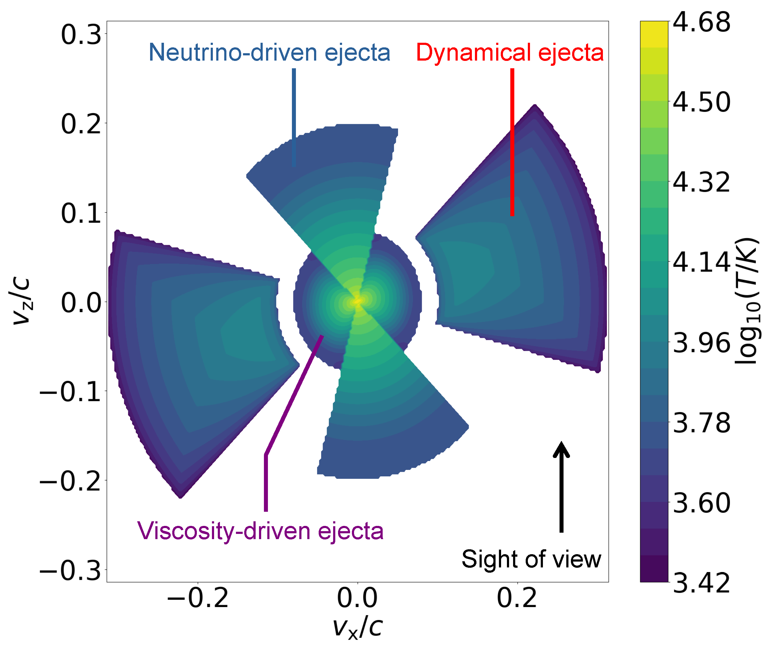
2.1. Kilonova
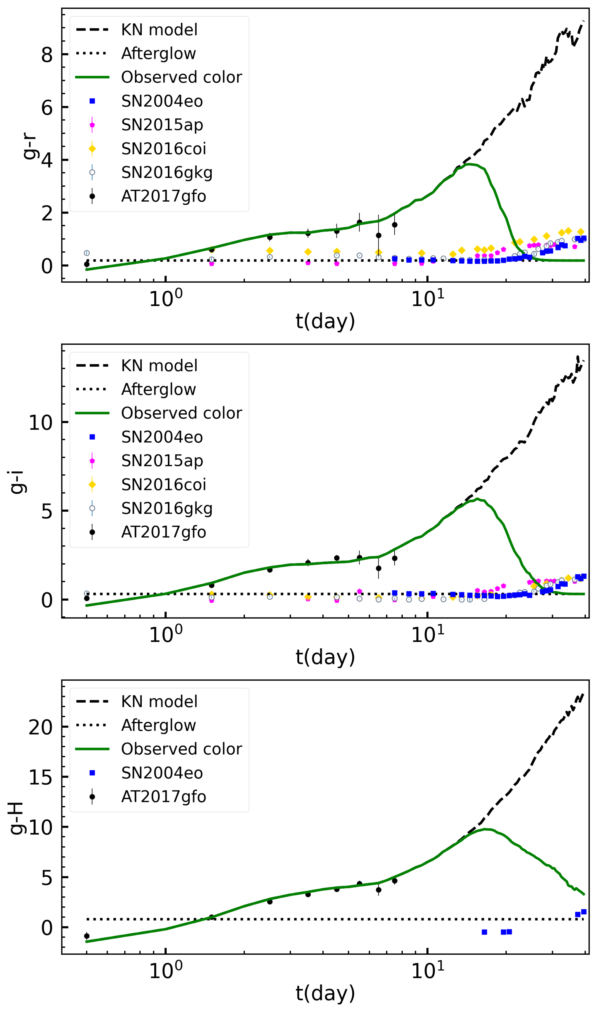
2.2. Afterglow
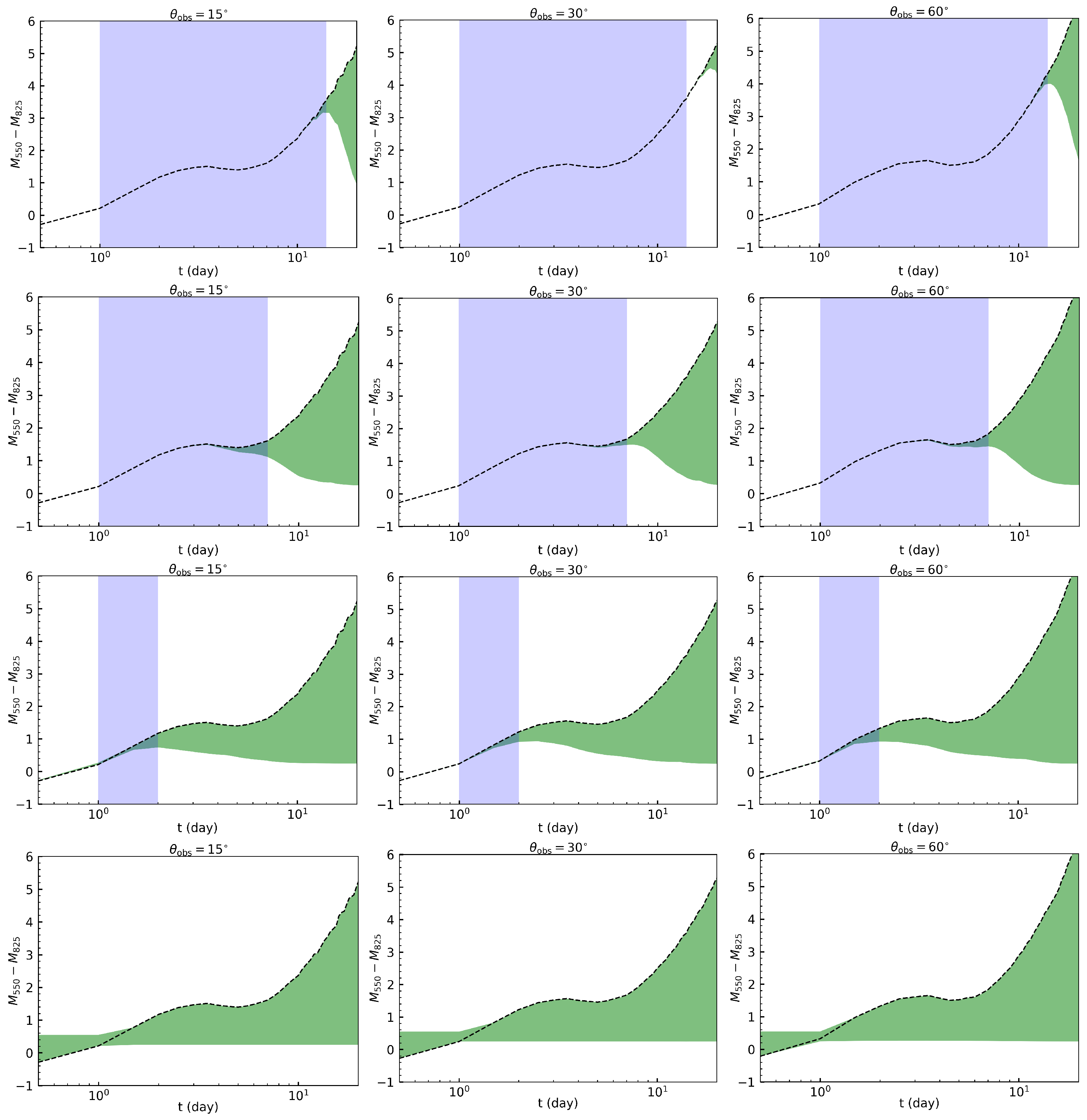
3. Results
3.1. SVOM VT
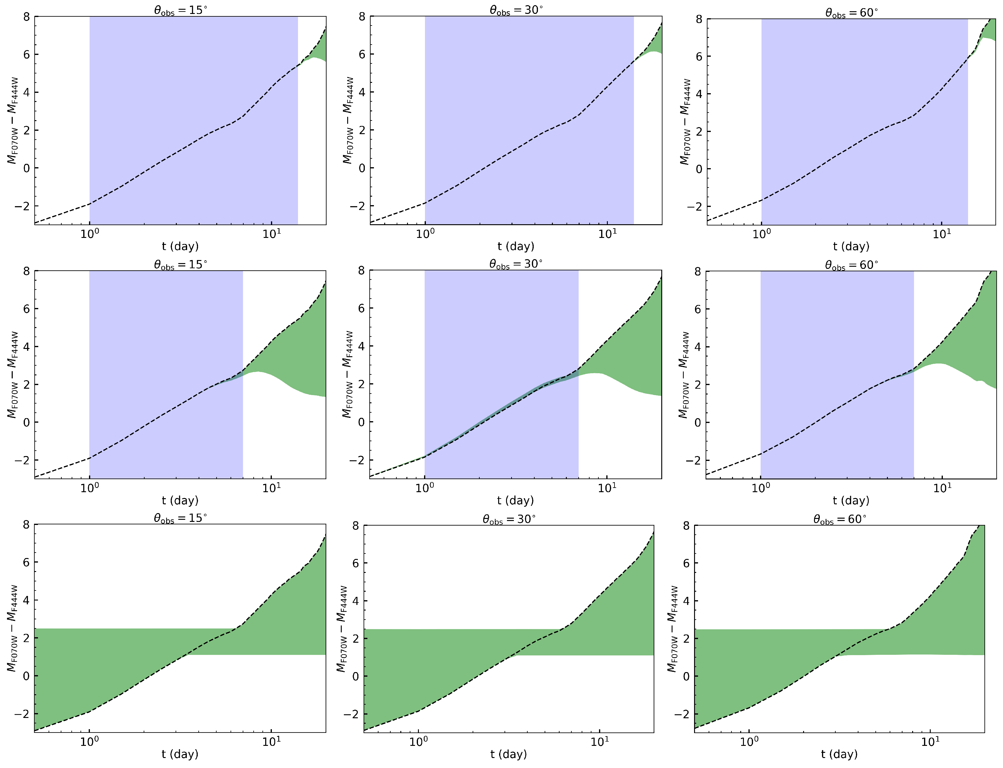
3.2. JWST NirCam
4. Discussion and Conclusions
Author Contributions
Funding
Data Availability Statement
Acknowledgments
Conflicts of Interest
Abbreviations
| SVOM | Space Multi-band Variable Object Monitor |
| VT | Visible Telescope |
| JWST | James Webb Space Telescope |
| NIRCam | Near-Infrared Camera |
| GRB | Gamma-ray burst |
| BH | Black hole |
| NS | Neutron star |
| BNS | Binary neutron stars |
| 1 | https://www.svom.eu/en/vt-visible-telescope-en accessed on 16 October 2024. |
| 2 | https://jwst-docs.stsci.edu/jwst-near-infrared-camera accessed on 16 October 2024. |
| 3 | http://tarot.obs-hp.fr/ accessed on 21 August 2023. |
| 4 | http://coatli.astroscu.unam.mx/ accessed on 21 August 2023. |
| 5 | http://ratir.astroscu.unam.mx/ accessed on 21 August 2023. |
References
- Fryer, C.L.; Woosley, S.E.; Hartmann, D.H. Formation Rates of Black Hole Accretion Disk Gamma-Ray Bursts. Astrophys. J. 1999, 526, 152–177. [Google Scholar] [CrossRef]
- Abbott, B.P.; Abbott, R.; Abbott, T.D.; Acernese, F.; Ackley, K.; Adams, C.; Adams, T.; Addesso, P.; Adhikari, R.X.; Adya, V.B.; et al. Multi-messenger Observations of a Binary Neutron Star Merger. Astrophys. J. Lett. 2017, 848, L12. [Google Scholar] [CrossRef]
- Li, L.X.; Paczyński, B. Transient Events from Neutron Star Mergers. Astrophys. J. Lett. 1998, 507, L59–L62. [Google Scholar] [CrossRef]
- Metzger, B.D.; Martínez-Pinedo, G.; Darbha, S.; Quataert, E.; Arcones, A.; Kasen, D.; Thomas, R.; Nugent, P.; Panov, I.V.; Zinner, N.T. Electromagnetic counterparts of compact object mergers powered by the radioactive decay of r-process nuclei. Mon. Not. R. Astron. Soc. 2010, 406, 2650–2662. [Google Scholar] [CrossRef]
- Bauswein, A.; Goriely, S.; Janka, H.T. Systematics of Dynamical Mass Ejection, Nucleosynthesis, and Radioactively Powered Electromagnetic Signals from Neutron-star Mergers. Astrophys. J. 2013, 773, 78. [Google Scholar] [CrossRef]
- Rosswog, S.; Korobkin, O.; Arcones, A.; Thielemann, F.K.; Piran, T. The long-term evolution of neutron star merger remnants—I. The impact of r-process nucleosynthesis. Mon. Not. R. Astron. Soc. 2014, 439, 744–756. [Google Scholar] [CrossRef]
- Abbott, R.; Abbott, T.D.; Acernese, F.; Ackley, K.; Adams, C.; Adhikari, N.; Adhikari, R.X.; Adya, V.B.; Affeldt, C.; Agarwal, D.; et al. Population of Merging Compact Binaries Inferred Using Gravitational Waves through GWTC-3. Phys. Rev. X 2023, 13, 011048. [Google Scholar] [CrossRef]
- Abbott, B.P.; Abbott, R.; Abbott, T.D.; Acernese, F.; Ackley, K.; Adams, C.; Adams, T.; Addesso, P.; Adhikari, R.X.; Adya, V.B.; et al. Estimating the Contribution of Dynamical Ejecta in the Kilonova Associated with GW170817. Astrophys. J. Lett. 2017, 850, L39. [Google Scholar] [CrossRef]
- Jin, Z.P.; Li, X.; Cano, Z.; Covino, S.; Fan, Y.Z.; Wei, D.M. The Light Curve of the Macronova Associated with the Long-Short Burst GRB 060614. Astrophys. J. Lett. 2015, 811, L22. [Google Scholar] [CrossRef]
- Jin, Z.P.; Hotokezaka, K.; Li, X.; Tanaka, M.; D’Avanzo, P.; Fan, Y.Z.; Covino, S.; Wei, D.M.; Piran, T. The Macronova in GRB 050709 and the GRB-macronova connection. Nat. Commun. 2016, 7, 12898. [Google Scholar] [CrossRef]
- Jin, Z.P.; Li, X.; Wang, H.; Wang, Y.Z.; He, H.N.; Yuan, Q.; Zhang, F.W.; Zou, Y.C.; Fan, Y.Z.; Wei, D.M. Short GRBs: Opening Angles, Local Neutron Star Merger Rate, and Off-axis Events for GRB/GW Association. Astrophys. J. 2018, 857, 128. [Google Scholar] [CrossRef]
- Jin, Z.P.; Covino, S.; Liao, N.H.; Li, X.; D’Avanzo, P.; Fan, Y.Z.; Wei, D.M. A kilonova associated with GRB 070809. Nat. Astron. 2020, 4, 77–82. [Google Scholar] [CrossRef]
- Troja, E.; Ryan, G.; Piro, L.; van Eerten, H.; Cenko, S.B.; Yoon, Y.; Lee, S.K.; Im, M.; Sakamoto, T.; Gatkine, P.; et al. A luminous blue kilonova and an off-axis jet from a compact binary merger at z = 0.1341. Nat. Commun. 2018, 9, 4089. [Google Scholar] [CrossRef] [PubMed]
- Troja, E.; Fryer, C.L.; O’Connor, B.; Ryan, G.; Dichiara, S.; Kumar, A.; Ito, N.; Gupta, R.; Wollaeger, R.T.; Norris, J.P.; et al. A nearby long gamma-ray burst from a merger of compact objects. Nature 2022, 612, 228–231. [Google Scholar] [CrossRef]
- Ascenzi, S.; Coughlin, M.W.; Dietrich, T.; Foley, R.J.; Ramirez-Ruiz, E.; Piranomonte, S.; Mockler, B.; Murguia-Berthier, A.; Fryer, C.L.; Lloyd-Ronning, N.M.; et al. A luminosity distribution for kilonovae based on short gamma-ray burst afterglows. Mon. Not. R. Astron. Soc. 2019, 486, 672–690. [Google Scholar] [CrossRef]
- Fong, W.; Laskar, T.; Rastinejad, J.; Escorial, A.R.; Schroeder, G.; Barnes, J.; Kilpatrick, C.D.; Paterson, K.; Berger, E.; Metzger, B.D.; et al. The Broadband Counterpart of the Short GRB 200522A at z = 0.5536: A Luminous Kilonova or a Collimated Outflow with a Reverse Shock? Astrophys. J. 2021, 906, 127. [Google Scholar] [CrossRef]
- Rastinejad, J.C.; Gompertz, B.P.; Levan, A.J.; Fong, W.f.; Nicholl, M.; Lamb, G.P.; Malesani, D.B.; Nugent, A.E.; Oates, S.R.; Tanvir, N.R.; et al. A kilonova following a long-duration gamma-ray burst at 350 Mpc. Nature 2022, 612, 223–227. [Google Scholar] [CrossRef]
- Levan, A.J.; Gompertz, B.P.; Salafia, O.S.; Bulla, M.; Burns, E.; Hotokezaka, K.; Izzo, L.; Lamb, G.P.; Malesani, D.B.; Oates, S.R.; et al. Heavy-element production in a compact object merger observed by JWST. Nature 2024, 626, 737–741. [Google Scholar] [CrossRef]
- Dai, C.Y.; Guo, C.L.; Zhang, H.M.; Liu, R.Y.; Wang, X.Y. Evidence for a Compact Stellar Merger Origin for GRB 230307A From Fermi-LAT and Multiwavelength Afterglow Observations. Astrophys. J. Lett. 2024, 962, L37. [Google Scholar] [CrossRef]
- Hotokezaka, K.; Nakar, E. Radioactive Heating Rate of r-process Elements and Macronova Light Curve. Astrophys. J. 2020, 891, 152. [Google Scholar] [CrossRef]
- Sneppen, A.; Watson, D.; Bauswein, A.; Just, O.; Kotak, R.; Nakar, E.; Poznanski, D.; Sim, S. Spherical symmetry in the kilonova AT2017gfo/GW170817. Nature 2023, 614, 436–439. [Google Scholar] [CrossRef] [PubMed]
- Heinzel, J.; Coughlin, M.W.; Dietrich, T.; Bulla, M.; Antier, S.; Christensen, N.; Coulter, D.A.; Foley, R.J.; Issa, L.; Khetan, N. Comparing inclination-dependent analyses of kilonova transients. Mon. Not. R. Astron. Soc. 2021, 502, 3057–3065. [Google Scholar] [CrossRef]
- Shrestha, M.; Bulla, M.; Nativi, L.; Markin, I.; Rosswog, S.; Dietrich, T. Impact of jets on kilonova photometric and polarimetric emission from binary neutron star mergers. Mon. Not. R. Astron. Soc. 2023, 523, 2990–3000. [Google Scholar] [CrossRef]
- Mészáros, P.; Rees, M.J. Optical and Long-Wavelength Afterglow from Gamma-Ray Bursts. Astrophys. J. 1997, 476, 232–237. [Google Scholar] [CrossRef]
- van Eerten, H.; van der Horst, A.; MacFadyen, A. Gamma-Ray Burst Afterglow Broadband Fitting Based Directly on Hydrodynamics Simulations. Astrophys. J. 2012, 749, 44. [Google Scholar] [CrossRef]
- Wang, H.; Dastidar, R.G.; Giannios, D.; Duffell, P.C. jetsimpy: A Highly Efficient Hydrodynamic Code for Gamma-Ray Burst Afterglow. Astrophys. J. Suppl. Ser. 2024, 273, 17. [Google Scholar] [CrossRef]
- Ryan, G.; van Eerten, H.; Piro, L.; Troja, E. Gamma-Ray Burst Afterglows in the Multimessenger Era: Numerical Models and Closure Relations. Astrophys. J. 2020, 896, 166. [Google Scholar] [CrossRef]
- Li, X.Y.; He, H.N.; Wei, D.M. On the Jet Structures of GRB 050820A and GRB 070125. Res. Astron. Astrophys. 2022, 22, 085021. [Google Scholar] [CrossRef]
- Zhu, Z.P.; Lei, W.H.; Malesani, D.B.; Fu, S.Y.; Liu, D.J.; Xu, D.; D’Avanzo, P.; Agüí Fernández, J.F.; Fynbo, J.P.U.; Gao, X.; et al. Optical and Near-infrared Observations of the Distant but Bright “New Year’s Burst” GRB 220101A. Astrophys. J. 2023, 959, 118. [Google Scholar] [CrossRef]
- Zhu, J.P.; Yang, Y.P.; Zhang, B.; Gao, H.; Yu, Y.W. Kilonova and Optical Afterglow from Binary Neutron Star Mergers. I. Luminosity Function and Color Evolution. Astrophys. J. 2022, 938, 147. [Google Scholar] [CrossRef]
- Bulla, M. POSSIS: Predicting spectra, light curves, and polarization for multidimensional models of supernovae and kilonovae. Mon. Not. R. Astron. Soc. 2019, 489, 5037–5045. [Google Scholar] [CrossRef]
- Granot, J.; Panaitescu, A.; Kumar, P.; Woosley, S.E. Off-Axis Afterglow Emission from Jetted Gamma-Ray Bursts. Astrophys. J. Lett. 2002, 570, L61–L64. [Google Scholar] [CrossRef]
- Totani, T.; Panaitescu, A. Orphan Afterglows of Collimated Gamma-Ray Bursts: Rate Predictions and Prospects for Detection. Astrophys. J. 2002, 576, 120–134. [Google Scholar] [CrossRef]
- Zou, Y.C.; Wu, X.F.; Dai, Z.G. Estimation of the detectability of optical orphan afterglows. Astron. Astrophys. 2007, 461, 115–119. [Google Scholar] [CrossRef]
- Ye, X.M.; Wei, D.M.; Zhu, Y.M.; Jin, Z.P. Optical Transient Source AT2021lfa: A Possible “Dirty Fireball”. Res. Astron. Astrophys. 2024, 24, 045011. [Google Scholar] [CrossRef]
- Huang, Y.F.; Dai, Z.G.; Lu, T. Failed gamma-ray bursts and orphan afterglows. Mon. Not. R. Astron. Soc. 2002, 332, 735–740. [Google Scholar] [CrossRef]
- Rhoads, J.E. Dirty Fireballs and Orphan Afterglows: A Tale of Two Transients. Astrophys. J. 2003, 591, 1097–1103. [Google Scholar] [CrossRef]
- Zhang, B. The Physics of Gamma-Ray Bursts; Cambridge University Press: Cambridge, UK, 2019. [Google Scholar]
- Fan, X.; Zou, G.; Wei, J.; Qiu, Y.; Gao, W.; Wang, W.; Yang, W.; Zhang, J.; Li, C.; Zhao, H.; et al. The Visible Telescope onboard the Chinese-French SVOM satellite. In Proceedings of the Space Telescopes and Instrumentation 2020: Optical, Infrared, and Millimeter Wave, Online, 14–22 December 2020; Society of Photo-Optical Instrumentation Engineers (SPIE) Conference Series. Lystrup, M., Perrin, M.D., Eds.; SPIE: Pamiers, France, 2020; Volume 11443, p. 114430Q. [Google Scholar] [CrossRef]
- Pan, Y.; Dan, L.; Sun, Z.; Huang, C.; Li, W.; Wang, F.; Zhao, H.; Zhang, J. Research on quantum efficiency calibration of SVOM VT CCDs. In Proceedings of the Applied Optics and Photonics China 2023 (AOPC2023), Beijing, China, 25–27 July 2023; Society of Photo-Optical Instrumentation Engineers (SPIE) Conference Series. Zhu, Y., Xue, S., Parker, Q., Eds.; SPIE: Pamiers, France, 2023; Volume 12965, p. 129650B. [Google Scholar] [CrossRef]
- Bartos, I.; Huard, T.L.; Márka, S. James Webb Space Telescope Can Detect Kilonovae in Gravitational Wave Follow-up Search. Astrophys. J. 2016, 816, 61. [Google Scholar] [CrossRef]
- Chen, M.H.; Liang, E.W. Radioactive decay of specific heavy elements as an energy source for late-time kilonovae and potential James Webb Space Telescope observations. Mon. Not. R. Astron. Soc. 2024, 527, 5540–5546. [Google Scholar] [CrossRef]
- Yang, Y.H.; Troja, E.; O’Connor, B.; Fryer, C.L.; Im, M.; Durbak, J.; Paek, G.S.H.; Ricci, R.; Bom, C.R.; Gillanders, J.H.; et al. A lanthanide-rich kilonova in the aftermath of a long gamma-ray burst. Nature 2024, 626, 742–745. [Google Scholar] [CrossRef]
- Gong, H.Y.; Wei, D.M.; Jin, Z.P.; Fan, Y.Z. Extension of semi-analytic kilonova model and the application in multicolour light curves fitting. Mon. Not. R. Astron. Soc. 2024, 531, 4422–4431. [Google Scholar] [CrossRef]
- Kasen, D.; Barnes, J. Radioactive Heating and Late Time Kilonova Light Curves. Astrophys. J. 2019, 876, 128. [Google Scholar] [CrossRef]
- Zhu, J.P.; Yang, Y.P.; Liu, L.D.; Huang, Y.; Zhang, B.; Li, Z.; Yu, Y.W.; Gao, H. Kilonova Emission from Black Hole-Neutron Star Mergers. I. Viewing-angle-dependent Lightcurves. Astrophys. J. 2020, 897, 20. [Google Scholar] [CrossRef]
- Perego, A.; Radice, D.; Bernuzzi, S. AT 2017gfo: An Anisotropic and Three-component Kilonova Counterpart of GW170817. Astrophys. J. Lett. 2017, 850, L37. [Google Scholar] [CrossRef]
- Piro, A.L.; Kollmeier, J.A. Evidence for Cocoon Emission from the Early Light Curve of SSS17a. Astrophys. J. 2018, 855, 103. [Google Scholar] [CrossRef]
- Wu, Z.; Ricigliano, G.; Kashyap, R.; Perego, A.; Radice, D. Radiation hydrodynamics modelling of kilonovae with SNEC. Mon. Not. R. Astron. Soc. 2022, 512, 328–347. [Google Scholar] [CrossRef]
- Banerjee, S.; Tanaka, M.; Kato, D.; Gaigalas, G.; Kawaguchi, K.; Domoto, N. Opacity of the Highly Ionized Lanthanides and the Effect on the Early Kilonova. Astrophys. J. 2022, 934, 117. [Google Scholar] [CrossRef]
- Wu, M.R.; Barnes, J.; Martínez-Pinedo, G.; Metzger, B.D. Fingerprints of Heavy-Element Nucleosynthesis in the Late-Time Lightcurves of Kilonovae. Phys. Rev. Lett. 2019, 122, 062701. [Google Scholar] [CrossRef] [PubMed]
- Barnes, J.; Kasen, D.; Wu, M.R.; Martínez-Pinedo, G. Radioactivity and Thermalization in the Ejecta of Compact Object Mergers and Their Impact on Kilonova Light Curves. Astrophys. J. 2016, 829, 110. [Google Scholar] [CrossRef]
- Pognan, Q.; Jerkstrand, A.; Grumer, J. On the validity of steady-state for nebular phase kilonovae. Mon. Not. R. Astron. Soc. 2022, 510, 3806–3837. [Google Scholar] [CrossRef]
- Radice, D.; Perego, A.; Hotokezaka, K.; Fromm, S.A.; Bernuzzi, S.; Roberts, L.F. Binary Neutron Star Mergers: Mass Ejection, Electromagnetic Counterparts, and Nucleosynthesis. Astrophys. J. 2018, 869, 130. [Google Scholar] [CrossRef]
- Waxman, E.; Ofek, E.O.; Kushnir, D.; Gal-Yam, A. Constraints on the ejecta of the GW170817 neutron star merger from its electromagnetic emission. Mon. Not. R. Astron. Soc. 2018, 481, 3423–3441. [Google Scholar] [CrossRef]
- Troja, E.; Piro, L.; van Eerten, H.; Wollaeger, R.T.; Im, M.; Fox, O.D.; Butler, N.R.; Cenko, S.B.; Sakamoto, T.; Fryer, C.L.; et al. The X-ray counterpart to the gravitational-wave event GW170817. Nature 2017, 551, 71–74. [Google Scholar] [CrossRef]
- Pastorello, A.; Mazzali, P.A.; Pignata, G.; Benetti, S.; Cappellaro, E.; Filippenko, A.V.; Li, W.; Meikle, W.P.S.; Arkharov, A.A.; Blanc, G.; et al. ESC and KAIT observations of the transitional Type Ia SN 2004eo. Mon. Not. R. Astron. Soc. 2007, 377, 1531–1552. [Google Scholar] [CrossRef]
- Prentice, S.J.; Ashall, C.; James, P.A.; Short, L.; Mazzali, P.A.; Bersier, D.; Crowther, P.A.; Barbarino, C.; Chen, T.W.; Copperwheat, C.M.; et al. Investigating the properties of stripped-envelope supernovae; what are the implications for their progenitors? Mon. Not. R. Astron. Soc. 2019, 485, 1559–1578. [Google Scholar] [CrossRef]
- Prentice, S.J.; Ashall, C.; Mazzali, P.A.; Zhang, J.J.; James, P.A.; Wang, X.F.; Vinkó, J.; Percival, S.; Short, L.; Piascik, A.; et al. SN 2016coi/ASASSN-16fp: An example of residual helium in a typeIc supernova? Mon. Not. R. Astron. Soc. 2018, 478, 4162–4192. [Google Scholar] [CrossRef]
- Becerra, R.L.; Klotz, A.; Atteia, J.L.; Guetta, D.; Watson, A.M.; De Colle, F.; Angulo-Valdez, C.; Butler, N.R.; Dichiara, S.; Fraija, N.; et al. Understanding the nature of the optical emission in gamma-ray bursts: Analysis from TAROT, COATLI, and RATIR observations. Mon. Not. R. Astron. Soc. 2023, 525, 3262–3273. [Google Scholar] [CrossRef]
- Villar, V.A.; Guillochon, J.; Berger, E.; Metzger, B.D.; Cowperthwaite, P.S.; Nicholl, M.; Alexander, K.D.; Blanchard, P.K.; Chornock, R.; Eftekhari, T.; et al. The Combined Ultraviolet, Optical, and Near-infrared Light Curves of the Kilonova Associated with the Binary Neutron Star Merger GW170817: Unified Data Set, Analytic Models, and Physical Implications. Astrophys. J. Lett. 2017, 851, L21. [Google Scholar] [CrossRef]
- Kyutoku, K.; Ioka, K.; Okawa, H.; Shibata, M.; Taniguchi, K. Dynamical mass ejection from black hole-neutron star binaries. Phys. Rev. D 2015, 92, 044028. [Google Scholar] [CrossRef]
- Kawaguchi, K.; Kyutoku, K.; Shibata, M.; Tanaka, M. Models of Kilonova/Macronova Emission from Black Hole-Neutron Star Mergers. Astrophys. J. 2016, 825, 52. [Google Scholar] [CrossRef]


| Parameters | Meanings | Values |
|---|---|---|
| Viewing angle in radians | ||
| Isotropic-equivalent energy in erg | [49,50,51,52,53,54] | |
| Half-opening angle of jet core in radians | [0.01,0.10,0.20,0.30] | |
| Circumburst density in cm−3 | [−4,−3,−2,−1,0,1] | |
| p | Electron energy distribution index | [2.1,2.2,2.3,2.4,2.5] |
| Energy fraction in electrons | [−3,−2,−1] | |
| Energy fraction in magnetic field | [−5,−4,−3,−2,−1] |
Disclaimer/Publisher’s Note: The statements, opinions and data contained in all publications are solely those of the individual author(s) and contributor(s) and not of MDPI and/or the editor(s). MDPI and/or the editor(s) disclaim responsibility for any injury to people or property resulting from any ideas, methods, instructions or products referred to in the content. |
© 2024 by the authors. Licensee MDPI, Basel, Switzerland. This article is an open access article distributed under the terms and conditions of the Creative Commons Attribution (CC BY) license (https://creativecommons.org/licenses/by/4.0/).
Share and Cite
Gong, H.; Wei, D.; Jin, Z. Off-Axis Color Characteristics of Binary Neutron Star Merger Events: Applications for Space Multi-Band Variable Object Monitor and James Webb Space Telescope. Universe 2024, 10, 403. https://doi.org/10.3390/universe10100403
Gong H, Wei D, Jin Z. Off-Axis Color Characteristics of Binary Neutron Star Merger Events: Applications for Space Multi-Band Variable Object Monitor and James Webb Space Telescope. Universe. 2024; 10(10):403. https://doi.org/10.3390/universe10100403
Chicago/Turabian StyleGong, Hongyu, Daming Wei, and Zhiping Jin. 2024. "Off-Axis Color Characteristics of Binary Neutron Star Merger Events: Applications for Space Multi-Band Variable Object Monitor and James Webb Space Telescope" Universe 10, no. 10: 403. https://doi.org/10.3390/universe10100403
APA StyleGong, H., Wei, D., & Jin, Z. (2024). Off-Axis Color Characteristics of Binary Neutron Star Merger Events: Applications for Space Multi-Band Variable Object Monitor and James Webb Space Telescope. Universe, 10(10), 403. https://doi.org/10.3390/universe10100403