Time-Delay Interferometry: The Key Technique in Data Pre-Processing Analysis of Space-Based Gravitational Waves

Abstract

Space gravitational wave detection primarily focuses on the rich wave sources corresponding to the millihertz frequency band, which provide key information for studying the fundamental physics of cosmology and astrophysics. However, gravitational wave signals are extremely weak, and any noise during the detection process could potentially overwhelm the gravitational wave signals. Therefore, data pre-processing is necessary to suppress the main noise sources. Among the various noise sources, laser phase noise is dominant, approximately seven orders of magnitude larger in strength than typical gravitational wave signals, and requires suppression using time-delay interferometry (TDI) techniques, which involve combining raw data with time delays. This paper will be based on the basic principles of TDI to present methods for obtaining multi-type TDI combinations, including algebraic methods for solving indeterminate equations and geometric methods for symbolic search. Furthermore, the applicability of TDI under actual operating conditions will be considered, such as the arm locking in conjunction with the TDI algorithm. Finally, the sensitivity functions for different types of TDI combinations will be provided, which can be used to evaluate the signal-to-noise ratio (SNRs) of different TDI combinations.

1. Introduction

Ground-based laser interferometric detectors are capable of detecting gravitational waves primarily in the hertz to kilohertz frequency range [1,2,3,4,5,6,7,8], making it difficult to detect important wave sources emitting low-frequency gravitational waves, which include galactic binaries, supermassive black hole binaries, and the stochastic early universe background, among others. Therefore, several space-based gravitational wave detection projects aimed at detecting the millihertz frequency band are being actively promoted, such as the LISA [9,10], TianQin [11] and Taiji [12] missions. The detection of low-frequency gravitational waves could help solve numerous issues in cosmology, astrophysics, and general relativity [13,14,15,16].

A typical space-based gravitational wave detector consists of three spacecraft forming an approximately equilateral triangle. It detects gravitational wave disturbances by measuring the Doppler shift in the laser exchange between two spacecraft separated by distances of ${10}^8$ to ${10}^9$ m. Compared to ground-based detectors, space-based gravitational wave detectors cannot maintain a constant distance between different arms, which results in residual noise after laser beat frequency being several orders of magnitude larger than the noise floor (test mass noise and optical path noise). Therefore, to achieve the required sensitivity, it is crucial to eliminate laser phase noise.

Currently, there are two technologies, arm locking [17,18,19] and TDI [20,21,22], that are used in successive steps to reduce the noise of pre-stabilized lasers (30 Hz/Hz^1/2). The arm locking technique will provide the second stage of laser stabilization, which attempts to convert the stability of the inter-spacecraft arm length into laser frequency stability through feedback control. The remaining laser phase noise is further eliminated in the post-processing stage using the TDI technique. TDI technique constructs a virtual equal-arm interferometer by applying appropriate delay operations and linear combinations to the measurement data. By combining arm locking with TDI, it will be achieved to suppress the laser phase noise to below the level of noise floor.

In 2003, Sheard et al., first proposed arm locking [17]. In 2008, Sutton et al., proposed dual arm locking, which uses common-mode and differential-mode interference information from two arms of different lengths to shift the zero point of the frequency response to outside the target frequency band [23]. However, the frequency pulling effect in the dual arm locking is significant, and in 2009, McKenzie et al. proposed a modified dual arm locking [24]. Within the frequency band below the first zero point of the frequency response, common-mode locking is used, while above the first zero point, dual arm locking is adopted. This arm locking mode combines the low-frequency pulling characteristics of common-mode locking with the high stability and gain advantages of dual arm locking.

The arm locking technique can suppress laser frequency noise by two to three orders of magnitude. To successfully detect gravitational wave signals, it is necessary to rely on a key technique in the data pre-processing stage: TDI. It constructs a virtual equal-arm configuration by time delaying and linearly combining the measurement data, thus differentially canceling noise. Tinto et al. first proposed the TDI technique in 1999 [20,21]. After more than 20 years of development, various methods have been developed to derive TDI combinations. These include algebraic methods [25,26] for solving constrained equations, geometric methods for symbolic search [27,28,29,30], as well as Matrix TDI [31], Bayesian TDI [32], and others. Various TDI combinations have been derived, such as the first-generation TDI combinations [20,21] that consider arm lengths as constant, the modified first-generation TDI combinations that account for constant arm lengths with rotation effects [33], and the second-generation TDI combinations that consider arm lengths varying over time [34]. Numerical validation and analysis have shown that the suppression capability of the second-generation TDI combinations meets the requirements for gravitational wave detection [35,36,37,38].

In addition to laser phase noise, other noises will also affect the detection of gravitational waves in space; for example, clock noise also needs to be suppressed by clock sideband comparison technology [39,40,41,42,43,44,45,46,47,48,49], which will not be a concern in this paper.

TDI and arm locking have been studied relatively independently. However, in actual space-based gravitational wave detection, the measurement data we obtain are after the application of arm locking. Therefore, it is crucial to develop a TDI technique that can perform delay operations on data streams containing controller parameters to suppress laser phase noise while preserving the gravitational wave signals.

Finally, to determine whether a detector can observe gravitational waves emitted by a specific source, it is necessary to analyze the sensitivity functions under different TDI combinations. Typically, the sensitivity of a detector can be quantified by the ratio of the response to a gravitational wave signal to the instrumental noise. This is referred to in the literature as the signal-to-oise ratio (SNR) and is usually presented in the frequency domain. There has been much discussion on the frequency dependence of the antenna response function for different polarizations and TDI combinations [50,51,52,53,54,55,56,57,58,59,60,61,62,63]. For equal-arm gravitational wave detectors, a semi-analytical formula of analytical expressions for the tensor mode [50] and semi-analytical formulae have been derived for all polarizations with different TDI combinations [54,55,56]. Simultaneously, numerical simulations have calculated the average response function of different TDI combinations to the six possible polarizations [57,58]. Recently, the full analytical formula for the tensor mode in the first-generation TDI Michelson combination was derived in [59]. However, a variety of TDI combinations can be used in the post-processing of space-based gravitational wave detection. To quickly and efficiently provide the sensitivity function for any TDI combination, we have provided the full analytical expressions for any TDI combination under different polarization modes [61,64].

The paper is organized as follows. In Section 2, we discuss the configuration of space-based gravitational wave detectors and the basic conventions for data streams. In Section 3, we present TDI combinations and analyze the principles of algebraic and geometric methods. Arm locking in conjunction with TDI is devived in Section 4. In Section 5, we analyze the sensitivity functions of different TDI combinations. The conclusion is given in Section 6.

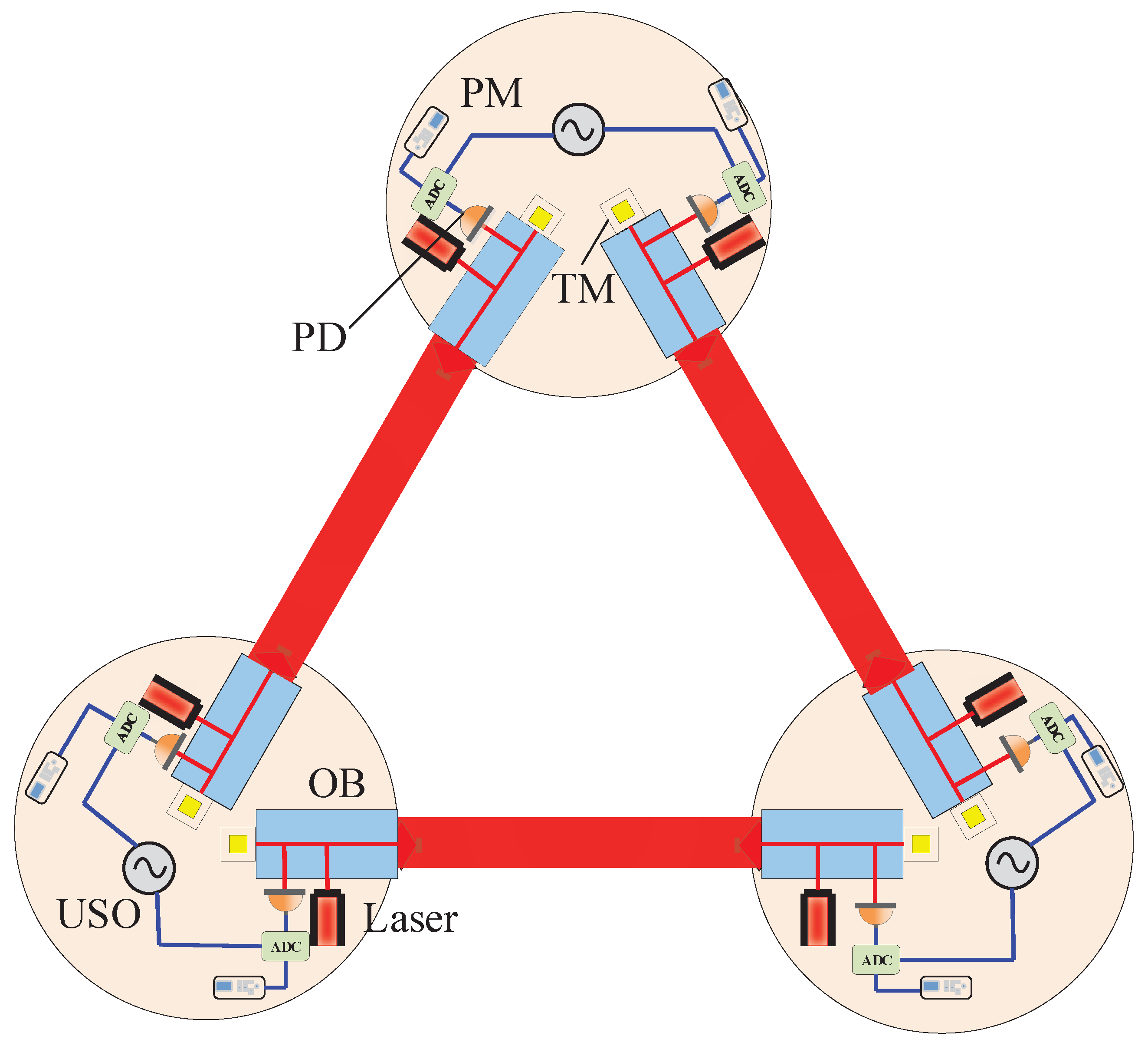
2. Conventions and Laser Interferometry Measurement Data

For a typical space-based gravitational wave detector, three spacecraft form an equilateral triangle. Each spacecraft emits lasers with a wavelength of 1064 nm to the other two spacecraft and receives lasers from them as well, as shown in Figure 1.

Each of the three spacecraft carries two nearly movable optical subassemblies (MOSAs), labeled i and $i^{\prime }(i=1,2,3)$. The detector arm lengths opposite to MOSAs i and $i^{\prime }$ are denoted as $L_i$ and $L_{i^{\prime }}$, respectively, depending on the direction of light propagation, which can be clockwise or counterclockwise (denoted with a prime) [22].

To facilitate the representation of the inter-spacecraft delay process experienced by time-varying, we first define six delay operators $D_i$, $D_{i^{\prime }}(i=1,2,3)$. These operators shift all time-dependent functions by the corresponding light travel times $L_i$, $L_{i^{\prime }}$, respectively. In this paper, we adopt the convention $c=1$, and for any data stream $f\left(t\right)$, we have

$$\begin{array}{c}\hfill \begin{array}{c}{D}_{i}f\left(t\right)=f(t-L_i\left(t\right)),\hfill \\ D_j{D}_{i}f\left(t\right)=D_{ji}f\left(t\right)=f(t-L_i(t-L_j)-L_j\left(t\right)).\hfill \end{array}\end{array}$$

(1)

Based on the principle of laser exchange between the three spacecraft, there are four different laser interferometric measurement data on each MOSA, which are as follows:

(a)

The incident laser from a distant spacecraft interferes with the local laser, with the incident laser carrying gravitational wave information. The signal obtained from this type of interference measurement is known as the scientific carrier interferometric data stream, denoted by $s_i^c\left(t\right)$.

(b)

The laser exchange between two adjacent MOSAs on the same spacecraft, where the laser from MOSA $i^{\prime }$ is transmitted through an optical fiber to the test mass of MOSA i and reflected to interfere with the local laser, resulting in the test mass interferometric data stream, is denoted by ${ϵ}_i\left(t\right)$.

(c)

The laser from the adjacent MOSA $i^{\prime }$ is transmitted through an optical fiber to MOSA i and beat with the local laser beam, yielding the reference interferometric data stream ${\tau }_i\left(t\right)$.

(d)

To eliminate clock noise, an electro-optic modulator is used to generate sidebands at both ends of the carrier. The driving frequency of the electro-optic modulator is referenced to the clock, transferring clock noise to the distant spacecraft. The sidebands are beat with each other to produce the sideband data stream $s_i^{sb}\left(t\right)$.

For simplicity, when considering the data streams on each spacecraft, we only take into account gravitational wave signals, laser frequency noise, clock noise, optical bench noise, test mass acceleration noise, fiber noise, and optical path noise.

On MOSA i, these are denoted as follows [45]:

$$\begin{array}{cc}\hfill s_i^c=& h_i+D_{i-1}{p}_{{(i+1)}^{\prime }}-p_i+N_i^{opt}-a_i{q}_i+\hfill \\ \hfill & 2\pi {\nu }_{{(i+1)}^{\prime }}\left[{\overrightarrow{n}}_{i-1}·D_{i-1}{\overrightarrow{\Delta }}_{{(i+1)}^{\prime }}+{\overrightarrow{n}}_{{(i-1)}^{\prime }}·{\overrightarrow{\Delta }}_i\right],\hfill \\ \hfill s_i^{sb}=& h_i+D_{i-1}{p}_{{(i+1)}^{\prime }}-p_i+N_i^{opt,sb}-c_i{q}_i-m_i{q}_i+\hfill \\ \hfill & 2\pi {\nu }_{{(i+1)}^{\prime }}\left[{\overrightarrow{n}}_{i-1}·D_{i-1}{\overrightarrow{\Delta }}_{{(i+1)}^{\prime }}+{\overrightarrow{n}}_{{(i-1)}^{\prime }}·{\overrightarrow{\Delta }}_i\right]+m_{{(i+1)}^{\prime }}{D}_{i-1}{q}_{i+1},\hfill \\ \hfill {\epsilon }_i=& p_{i^{\prime }}-p_i+{\mu }_{i^{\prime }}-4\pi {\nu }_{i^{\prime }}\left[{\overrightarrow{n}}_{{(i-1)}^{\prime }}·{\overrightarrow{\delta }}_i-{\overrightarrow{n}}_{{(i-1)}^{\prime }}·{\overrightarrow{\Delta }}_i\right]-b_i{q}_i,\hfill \\ \hfill {\tau }_i=& p_{i^{\prime }}-p_i+{\mu }_{i^{\prime }}-b_i{q}_i.\hfill \end{array}$$

(2)

On MOSA $i^{\prime }$, we have

$$\begin{array}{cc}\hfill s_{i^{\prime }}^c=& h_{i^{\prime }}+D_{{(i+1)}^{\prime }}{p}_{i-1}-p_{i^{\prime }}+N_{i^{\prime }}^{opt}-a_{i^{\prime }}{q}_{i^{\prime }}+\hfill \\ \hfill & 2\pi {\nu }_{i-1}\left[{\overrightarrow{n}}_{i+1}·D_{{(i+1)}^{\prime }}{\overrightarrow{\Delta }}_{i-1}+{\overrightarrow{n}}_{i+1}·{\overrightarrow{\Delta }}_{i^{\prime }}\right],\hfill \\ \hfill s_{i^{\prime }}^{sb}=& h_{i^{\prime }}+D_{{(i+1)}^{\prime }}{p}_{i-1}-p_{i^{\prime }}+N_{i^{\prime }}^{opt,sb}-c_{i^{\prime }}{q}_i-m_{i^{\prime }}{q}_i+\hfill \\ \hfill & 2\pi {\nu }_{i-1}\left[{\overrightarrow{n}}_{{(i+1)}^{\prime }}·D_{{(i+1)}^{\prime }}{\overrightarrow{\Delta }}_{i-1}+{\overrightarrow{n}}_{i+1}·{\overrightarrow{\Delta }}_{i^{\prime }}\right]+m_{i-1}{D}_{{(i+1)}^{\prime }}{q}_{i-1},\hfill \\ \hfill {\epsilon }_{i^{\prime }}=& p_i-p_{i^{\prime }}+{\mu }_i-4\pi {\nu }_{i^{\prime }}\left[{\overrightarrow{n}}_{i+1}·{\overrightarrow{\delta }}_{i^{\prime }}-{\overrightarrow{n}}_{i+1}·{\overrightarrow{\Delta }}_{i^{\prime }}\right]-b_{i^{\prime }}{q}_i,\hfill \\ \hfill {\tau }_{i^{\prime }}=& p_i-p_{i^{\prime }}+{\mu }_i-b_{i^{\prime }}{q}_i,\hfill \end{array}$$

(3)

where $h_i$ represents the gravitational wave signal, $p_i$ denotes the laser phase noise, ${\nu }_i$ is the center frequency of the laser, ${\overrightarrow{\Delta }}_i$ refers to the optical bench noise, $N_i^{opt}$ represents the optical path noise, $q_i$ stands for the clock noise, ${\mu }_i$ denotes the fiber noise, ${\overrightarrow{\delta }}_i$ represents the test mass acceleration noise, and $m_i$ is the modulation factor.

The conversion coefficients $a_{i,i^{\prime }}$, $b_{i,i^{\prime }}$, $c_{i,i^{\prime }}$ are defined as

$$\begin{array}{cc}\hfill a_i& ={\displaystyle \frac{{\nu }_{{(i+1)}^{\prime }}\left(1-{\dot{L}}_{i-1}\right)-{\nu }_i}{f_i}},a_{i^{\prime }}={\displaystyle \frac{{\nu }_{i-1}\left(1-{\dot{L}}_{{(i+1)}^{\prime }}\right)-{\nu }_{i^{\prime }}}{f_i}},\hfill \\ \hfill b_i& ={\displaystyle \frac{{\nu }_{i^{\prime }}-{\nu }_i}{f_i}},b_{i^{\prime }}={\displaystyle \frac{{\nu }_i-{\nu }_{i^{\prime }}}{f_i}}=-b_i,\hfill \\ \hfill c_i& ={\displaystyle \frac{\left({\nu }_{{(i+1)}^{\prime }}+m_{{(i+1)}^{\prime }}{f}_{i+1}\right)\left(1-{\dot{L}}_{i-1}\right)-\left({\nu }_i+m_i{f}_i\right)}{f_i}},\hfill \\ \hfill c_{i^{\prime }}& ={\displaystyle \frac{\left({\nu }_{i-1}+m_{i-1}{f}_{i-1}\right)\left(1-{\dot{L}}_{{(i+1)}^{\prime }}\right)-\left({\nu }_{i^{\prime }}+m_{i^{\prime }}{f}_i\right)}{f_i}},\hfill \end{array}$$

(4)

where $f_i$ is the clock frequency.

To process the output data from the instrument, the first step is to eliminate the optical bench noise. To do this, intermediate variables are introduced [45]:

$$\begin{array}{cc}\hfill {\xi }_i\equiv & s_i^{\mathrm{c}}-{\displaystyle \frac{{\nu }_{{(i+1)}^{\prime }}}{{\nu }_{i^{\prime }}}}{\displaystyle \frac{{\epsilon }_i-{\tau }_i}{2}}-{\displaystyle \frac{{\nu }_{{(i+1)}^{\prime }}}{{\nu }_{i+1}}}{\displaystyle \frac{D_{i-1}{\epsilon }_{{(i+1)}^{\prime }}-D_{i-1}{\tau }_{{(i+1)}^{\prime }}}{2}},\hfill \\ \hfill {\xi }_{i^{\prime }}\equiv & s_{i^{\prime }}^{\mathrm{c}}-{\displaystyle \frac{{\nu }_{i-1}}{{\nu }_i}}{\displaystyle \frac{{\epsilon }_{i^{\prime }}-{\tau }_{i^{\prime }}}{2}}-{\displaystyle \frac{{\nu }_{i-1}}{{\nu }_{{(i-1)}^{\prime }}}}{\displaystyle \frac{D_{{(i+1)}^{\prime }}{\epsilon }_{i-1}-D_{{(i+1)}^{\prime }}{\tau }_{i-1}}{2}}.\hfill \end{array}$$

(5)

To eliminate the laser phase noise with a prime, additional intermediate variables are defined as

$$\begin{array}{cc}\hfill & {\eta }_i\equiv {\xi }_i-D_{i-1}{z}_{i+1},\hfill \\ \hfill & {\eta }_{i^{\prime }}\equiv {\xi }_{i^{\prime }}+z_i,\hfill \end{array}$$

(6)

where

$$z_i\equiv {\displaystyle \frac{({\tau }_i-{\tau }_{i^{\prime }})}{2}}.$$

(7)

Combining Equations (2)–(7), the data for each spacecraft are [45,46]

$$\begin{array}{cc}\hfill {\eta }_i=& h_i+D_{i-1}{p}_{i+1}-p_i-a_i{q}_i+D_{i-1}{b}_{i+1}{q}_{i+1}+N_i^{oms}\hfill \\ \hfill & +2\pi {\nu }_{{(i+1)}^{\prime }}{\overrightarrow{n}}_{i-1}\left[D_{i-1}{\overrightarrow{\delta }}_{{(i+1)}^{\prime }}-{\overrightarrow{\delta }}_i\right],\hfill \\ \hfill {\eta }_{i^{\prime }}=& h_{i^{\prime }}+D_{{(i+1)}^{\prime }}{p}_{i-1}-p_i+\left(b_{i^{\prime }}-a_{i^{\prime }}\right)q_i+N_{i^{\prime }}^{oms}\hfill \\ \hfill & +2\pi {\nu }_{i-1}{\overrightarrow{n}}_{i+1}·\left[{\overrightarrow{\delta }}_i-D_{{(i+1)}^{\prime }}{\overrightarrow{\delta }}_{i-1}\right].\hfill \end{array}$$

(8)

Equation (8) assumes that the fiber noise is reciprocal.

3. Time Delay Interferometry Technique for Reducing Laser Phase Noise

This section first introduces the basic principles of TDI using the Michelson interferometer as an example and then extends the concept to the split interferometry configuration corresponding to space-based gravitational wave detectors. Finally, it presents the algebraic and geometric methods for obtaining TDI combinations.

3.1. The Basic Principles of TDI

TDI is a post-processing technique that constructs virtual equal-arm interferometers by time-delaying and recombining data. As shown in Figure 2a, in an unequal-arm Michelson interferometer, the laser is split and then travels through two unequal arms of lengths $L_1$ and $L_2$, respectively, before interfering with the local laser. The interference data obtained by the two photoelectric detectors (considering only laser phase noise) can be represented as

$$\begin{array}{c}\hfill \begin{array}{c}{y}_{\mathrm{PD},1}\left(t\right)=p\left(t-2L_1\right)-p\left(t\right),\hfill \\ y_{\mathrm{PD},2}\left(t\right)=p\left(t-2L_2\right)-p\left(t\right).\hfill \end{array}\end{array}$$

(9)

Due to the unequal arm lengths, there is residual laser phase noise after differencing the two interference signals:

$$\begin{array}{c}\hfill \begin{array}{c}{y}_{\mathrm{PD},1}\left(t\right)-y_{\mathrm{PD},2}\left(t\right)=p\left(t-2L_1\right)-p\left(t-2L_2\right).\hfill \end{array}\end{array}$$

(10)

If the two interference data are each delayed and then differenced, the residual laser phase noise will be

$$\begin{array}{c}\hfill \begin{array}{c}{y}_{\mathrm{PD},1}\left(t-2L_2\right)-y_{\mathrm{PD},2}\left(t-2L_1\right)=p\left(t-2L_1\right)-p\left(t-2L_2\right).\hfill \end{array}\end{array}$$

(11)

By comparing the difference signal of the measurement data from Equation (10) with the difference signal of the delayed data from Equation (11), it can be observed that the laser phase fluctuations have the same temporal structure.

Therefore, by subtracting Equation (10) from Equation (11), a new data set without laser phase noise can be constructed, given by

$$\begin{array}{cc}\hfill X\left(t\right):=& \left[y_{\mathrm{PD},1}\left(t-2L_2\right)-y_{\mathrm{PD},2}\left(t-2L_1\right)\right]\hfill \\ \hfill & -\left[y_{\mathrm{PD},1}\left(t\right)-y_{\mathrm{PD},2}\left(t\right)\right],\hfill \end{array}$$

(12)

To better understand the principle of TDI from a physical perspective, the above combination $X\left(t\right)$ can be rewritten as

$$\begin{array}{cc}\hfill X\left(t\right):=& \left[y_{\mathrm{PD},2}\left(t\right)+y_{\mathrm{PD},1}(t-2L_2)\right]\hfill \\ \hfill & -\left[y_{\mathrm{PD},1}\left(t\right)+y_{\mathrm{PD},2}(t-2L_1)\right].\hfill \end{array}$$

(13)

The laser propagation path constructed by Equation (13) is shown in Figure 2b. The first bracket corresponds to the blue solid line path in the figure, and the second bracket corresponds to the black dashed line path.

In the case where the optical instruments are fixed, both laser beams travel the same optical path, so the laser phase noise is exactly canceled out by differencing. The path shown in Figure 2b is a virtually synthesized path in the data post-processing, and it is not a “real” path. TDI technique can achieve the equal-arm interferometry that is physically difficult to implement in space-based gravitational wave detection [33].

In space-based gravitational wave detection, applying delay and then translation to Equation (8) constructs a virtual equal-arm interferometer, and its general expression is

$$\begin{array}{c}\hfill \mathrm{TDI}=\sum _{i=1}^3(P_i{\eta }_i+P_{i^{\prime }}{\eta }_{i^{\prime }}),\end{array}$$

(14)

where $P_i$ and $P_{i^{\prime }}$ represent the polynomial coefficients of the time delay operator. For instance, for the first-generation Michelson combination, the expression is

$$\begin{array}{c}\hfill X_1=({\mathcal{D}}_{2^{\prime }23}{\eta }_{2^{\prime }}+{\mathcal{D}}_{2^{\prime }2}{\eta }_1+{\mathcal{D}}_{2^{\prime }}{\eta }_3+{\eta }_{1^{\prime }})-({\mathcal{D}}_{{33}^{\prime }{2}^{\prime }}{\eta }_3+{\mathcal{D}}_{{33}^{\prime }}{\eta }_{1^{\prime }}+{\mathcal{D}}_3{\eta }_{2^{\prime }}+{\eta }_1).\end{array}$$

(15)

The corresponding polynomial coefficients are:

$$\begin{array}{cc}\hfill P_1=& -1+D_{2^{\prime }2},\hfill \\ \hfill P_2=& 0,\hfill \\ \hfill P_3=& D_{2^{\prime }}-D_{{33}^{\prime }{2}^{\prime }},\hfill \\ \hfill P_{1^{\prime }}=& 1-D_{{33}^{\prime }},\hfill \\ \hfill P_{2^{\prime }}=& D_{2^{\prime }23}-D_3,\hfill \\ \hfill P_{3^{\prime }}=& 0.\hfill \end{array}$$

The synthesized photon trajectory is as shown in Figure 3.

3.2. Methods for Obtaining TDI Combinations

Currently, there are two methods for obtaining TDI combinations: the algebraic method of solving constraint equations and the geometric method of symbolic search. These two methods complement each other, opening up entirely different avenues for presenting multiple types of TDI combinations. Below, the algebraic and geometric methods for obtaining TDI combinations will be introduced respectively.

3.2.1. Algebraic Method

The algebraic method for solving TDI combinations involves calculating the linear system of equations formed by the time delay operators [25,26]. Therefore, the commutativity of the time delay operators directly affects the solving process. The starting point for solving TDI combinations using the algebraic method is the following equation:

$$\begin{array}{cc}\hfill & P_1+P_{1^{\prime }}-P_{2^{\prime }}{D}_{3^{\prime }}-P_3{D}_2=0,\hfill \\ \hfill & P_2+P_{2^{\prime }}-P_{3^{\prime }}{D}_{1^{\prime }}-P_1{D}_3=0,\hfill \\ \hfill & P_3+P_{3^{\prime }}-P_{1^{\prime }}{D}_{2^{\prime }}-P_2{D}_1=0.\hfill \end{array}$$

(16)

This equation is one with six unknowns and three variables. By performing Gaussian elimination on it, we obtain

$$\begin{array}{cc}\hfill & P_3(1-D_{231})+P_{1^{\prime }}(D_{31}-D_{2^{\prime }})+\hfill \\ \hfill & P_{2^{\prime }}(D_1-D_{3^{\prime }31})+P_{3^{\prime }}(1-D_{1^{\prime }1})=0,\hfill \end{array}$$

(17)

This equation does not introduce any assumptions regarding the commutativity of the time delay operators. Clearly, the solution space of equation Equation (17) is completely equivalent to the solution space of equation Equation (16). The solution of the first-generation TDI and the modified first-generation TDI for Equation (17) is entirely similar. For the first-generation TDI combination, Equation (17) satisfies

$$\begin{array}{cc}\hfill & (1-D_{123})P_3+(D_{13}-D_2)P_{1^{\prime }}+\hfill \\ \hfill & D_1(1-D_{33})P_{2^{\prime }}+(1-D_{11})P_{3^{\prime }}=0.\hfill \end{array}$$

(18)

This equation is one located in the polynomial ring over three variables $D_1$, $D_2$, $D_3$. More specifically, what we are solving now is the first constraint module over the polynomial ring. The solving process is completed by calculating the Groebner basis of the ideal I, which is defined as [25]:

$$\begin{array}{c}\hfill I=\{1-D_{123},D_{13}-D_2,D_1(1-D_{33}),1-D_{11}\}.\end{array}$$

(19)

Now there are many software packages that can directly perform such calculations, for example, Mathematica. Through this set of methods in commutative algebra, the basis vectors of the solution space for the first-generation TDI can be obtained [25].

For the modified first-generation TDI combinations, what needs to be considered is the polynomial ring over six variables $D_1$, $D_2$, $D_3$, $D_{1^{\prime }}$, $D_{2^{\prime }}$, $D_{3^{\prime }}$ [26].

However, when considering the second-generation and modified second-generation TDI, the commutativity of the delay operators is destroyed, which prevents the use of the aforementioned similar methods.

Mathematically speaking, in non-commutative situations, the termination condition for the Groebner basis algorithm may not necessarily exist. For this reason, the “combinatorial algebra method” has been developed in [65].

3.2.2. Geometric Method

The trajectory of TDI can be intuitively characterized by a spacetime diagram, as shown in Figure 4. The horizontal direction represents the satellite number, while the vertical direction represents the time axis.

Two virtual laser links (blue solid line and orange dashed line) start from the black square at time −4 (−8) and converge at the black circle at time 0, exactly forming a closed loop. To clearly describe the propagation of the laser between spacecraft, the spacecraft numbers in the horizontal axis direction can be expandably arranged sequentially. Throughout the entire closed loop of the TDI combination, the accumulated light propagation time must be 0. For an n-link TDI combination, the search may be $2^n\times 2^n$. The direction of laser propagation and the direction of the time axis can be represented by specific numbers, 0 and 1. For example, laser propagation in a clockwise direction is denoted as 1, while counterclockwise propagation is denoted as 0. When the laser beam propagates between two satellites along the direction of the time axis, it is denoted as 1, and against the time axis direction, it is denoted as 0. In fact, in the geometric spacetime diagram, when the previous link is determined, there are three possible choices for the propagation direction of the current laser link between spacecraft and the time direction. Therefore, to reduce the search time, we use a ternary symbolic search algorithm to find TDI combinations. This method combines the two degrees of freedom of the laser propagation direction between spacecraft and the time sequence direction, with the convention of using 0, 1, and 2. Each link will have three possible choices.

Assuming a $2n$-link example, we first analyze the left n links and then consider the right n links.

By default, the first detector arm is from spacecraft i to spacecraft $i+1$, and the search for the minimum value is

$$3^{n-1}=\left\{1,\underset{n-1}{\underbrace{0,\dots 0}}\right\},$$

(20)

The maximum value is

$$\begin{array}{c}\hfill 2\times 3^{n-1}-1=\left\{1,\underset{n-1}{\underbrace{2,\dots 2}}\right\}.\end{array}$$

(21)

After the spacecraft and time parameters are defined, the search is conducted by accumulating the time and spacecraft numbers.

Next, the arm length and its rate of change are further defined. Twelve empty sets are provided to store six data points under the positive time sequence and six under the negative time sequence, and the data at a certain moment are stored. Based on the constraints of the TDI virtual equal-arm condition, a judgment is made. After all TDI combinations are found, it is necessary to screen and check whether two combinations are the same at a fixed zero point to eliminate duplicates. We use a ternary algorithm, which has resulted in the search for 45 s-generation TDI combinations. Their spacetime diagrams and trajectories are presented in the literature [30,66].

4. Arm Locking in Conjunction with Time-Delay Interferometry

4.1. The Principle of Arm Locking

We first briefly review the principle of arm locking by considering the simplest scenario, which involves only a single arm [17]. As shown in Figure 5, the light emanated from the master laser is split into two parts. The signal travels along the arm to reach the distant spacecraft, where the slave laser’s phase is locked to the incoming beam and then sends the beam back to the master spacecraft.

The interference between the two laser beams is implemented by a negative feedback, and the output of the phasemeter can be expressed as

$$\begin{array}{c}\hfill {\varphi }_{\mathrm{PM}}\left(t\right)=p\left(t\right)-\mathcal{D}p\left(t\right)=p\left(t\right)-p\left(t-\tau \right).\end{array}$$

(22)

To determine the transfer function from the input phase noise to the phasemeter output of the interferometer, Equation (22) is transformed into the frequency domain form:

$$\begin{array}{c}\hfill {\varphi }_{\mathrm{PM}}\left(s\right)=p\left(s\right)-p\left(s\right)e^{-s\tau }=T\left(s\right)p\left(s\right)\end{array}$$

(23)

in the s-domain, where

$$\begin{array}{c}\hfill T\left(s\right)=1-e^{-s\tau }\end{array}$$

(24)

is the transfer function.

In actual application, two controllers, denoted as $G_1$ and $G_2$, are integrated into the optical feedback path to mitigate laser phase noise [17]. For example, the effective transfer function given by Equation (24) for the subloop incorporating controller $G_2$ is subsequently altered to the following expression.

$$\begin{array}{c}\hfill T_1\left(s\right)=1-{\displaystyle \frac{G_2\left(s\right)}{1+G_2\left(s\right)}}{e}^{-s\tau }.\end{array}$$

(25)

Finally, the output of the closed-loop signal is

$$\begin{array}{c}\hfill \varphi \left(s\right)={\displaystyle \frac{p_1\left(s\right)}{1+L_1\left(s\right)}}+{\displaystyle \frac{G_1\left(s\right)p_2\left(s\right)}{\left(1+G_2\left(s\right)\right)\left(1+L_1\left(s\right)\right)}},\end{array}$$

(26)

where

$$\begin{array}{c}\hfill L_1\left(s\right)=[1-{\displaystyle \frac{G_2\left(s\right)}{1+G_2\left(s\right)}}{e}^{-s\tau }]G_1\left(s\right)=T_1\left(s\right)G_1\left(s\right)\end{array}$$

(27)

gives the open-loop transfer function for the master laser.

In the above discussions, we have primarily focused on the laser phase noise p. Equation (26) reveals that the laser phase noise is suppressed, but at the frequency of $\omega ={\displaystyle \frac{1}{n\tau }}$, where the transfer function equals 0, there is a response singularity, and the noise cannot be suppressed at these frequencies. To address this issue, it is necessary to employ a modified dual-arm locking scheme [24].

4.2. Transformation Definition

Mathematically, one effectively modifies the definitions of the TDI variables in Equation (8) as follows:

$$\begin{array}{cc}\hfill {\eta }_i=& {\mathcal{D}}_{i-1}\left[p_{i+1}+{\delta }_{{(i+1)}^{\prime }}\right]-\left[p_i+{\delta }_i\right]+2{\delta }_i+N_i^{opt}+h_i,\hfill \end{array}$$

(28a)

$$\begin{array}{cc}\hfill {\eta }_{i^{\prime }}=& {\mathcal{D}}_{{(i+1)}^{\prime }}\left[p_{i-1}+{\delta }_{i-1}\right]-\left[p_i+{\delta }_{i^{\prime }}\right]+2{\delta }_{i^{\prime }}+N_{i^{\prime }}^{opt}+h_{i^{\prime }}.\hfill \end{array}$$

(28b)

Here, we have not taken clock noise into account and have introduced the shorthands:

$$\begin{array}{cc}\hfill {\delta }_i=& 2\pi {\nu }_{i^{\prime }}{\overrightarrow{n}}_{{(i-1)}^{\prime }}·{\overrightarrow{\delta }}_i,\hfill \\ \hfill {\Delta }_i=& 2\pi {\nu }_{i^{\prime }}{\overrightarrow{n}}_{{(i-1)}^{\prime }}·{\overrightarrow{\Delta }}_i,\hfill \\ \hfill {\delta }_{i^{\prime }}=& 2\pi {\nu }_i{\overrightarrow{n}}_{i+1}·{\overrightarrow{\delta }}_{i^{\prime }},\hfill \\ \hfill {\Delta }_{i^{\prime }}=& 2\pi {\nu }_i{\overrightarrow{n}}_{i+1}·{\overrightarrow{\Delta }}_{i^{\prime }}.\hfill \end{array}$$

(29)

The physical quantities in the data stream of the above equation are replaced by variables, and the equivalent laser frequency noise, test mass noise, and optical path noise are described as follows:

$$\begin{array}{cc}\hfill {\tilde{\eta }}_i\equiv & -{\eta }_i,\hfill \\ \hfill {\tilde{p}}_i\equiv & p_i+{\delta }_i,\hfill \\ \hfill {\tilde{\delta }}_i\equiv & {\delta }_{i^{\prime }}-{\delta }_i,\hfill \\ \hfill {\tilde{h}}_i\equiv & 2{\delta }_i+N_i^{opt}+h_i,\hfill \\ \hfill {\tilde{h}}_{i^{\prime }}\equiv & 2{\delta }_{i^{\prime }}+N_{i^{\prime }}^{opt}+h_{i^{\prime }},\hfill \end{array}$$

(30)

where

$$\begin{array}{cc}\hfill {\tilde{p}}_{i^{\prime }}\equiv & p_{i^{\prime }}+{\delta }_{i^{\prime }}={\tilde{p}}_i+{\tilde{\delta }}_i\hfill \end{array}$$

is implied. By using Equation (30), Equations (28a) and (28b) can be rewritten as

$$\begin{array}{cc}\hfill {\tilde{\eta }}_i=& {\tilde{p}}_i-{\mathcal{D}}_{i-1}\left({\tilde{p}}_{(i+1)}+{\tilde{\delta }}_{i+1}\right)-{\tilde{h}}_i,\hfill \end{array}$$

(31a)

$$\begin{array}{cc}\hfill {\tilde{\eta }}_{i^{\prime }}=& \left({\tilde{p}}_i+{\tilde{\delta }}_i\right)-{\mathcal{D}}_{{(i+1)}^{\prime }}{\tilde{p}}_{(i-1)}-{\tilde{h}}_{i^{\prime }},\hfill \end{array}$$

(31b)

By utilizing the simple convention of Equations (31a) and (31b), er can derive six data streams under the arm locking mode.

Based on the expressions in [67] and by employing certain approximations, the following data stream can be obtained as

$$\begin{array}{cc}\hfill {\tilde{\eta }}_1\approx & {\displaystyle \frac{{\tilde{p}}_1}{2G_1}}\left(1-e^{-s\tau }\right)\hfill \\ \hfill -& {\displaystyle \frac{1}{2}}\left({\displaystyle \frac{({\tilde{p}}_2+{\tilde{\delta }}_2)e^{-\frac{s}{2}\tau }}{G_2}}-{\displaystyle \frac{{\tilde{p}}_3{e}^{-\frac{s}{2}\tau }}{G_3}}\right)\left(1-{\displaystyle \frac{1}{s\Delta \tau }}\right)\left(1-e^{-s\tau }\right)\hfill \\ \hfill +& {\displaystyle \frac{1}{2}}\left(-{\tilde{h}}_{2^{\prime }1}+{\tilde{h}}_{{31}^{\prime }}-{\tilde{\delta }}_1\left(1-e^{-s\tau }\right)\right)\left(1-{\displaystyle \frac{1}{s\Delta \tau }}\right)\left(1-e^{-s\tau }\right),\hfill \end{array}$$

(32)

$$\begin{array}{cc}\hfill {\tilde{\eta }}_{1^{\prime }}\approx & {\displaystyle \frac{{\tilde{p}}_1}{2G_1}}\left(1-e^{-s\tau }\right)\hfill \\ \hfill +& {\displaystyle \frac{1}{2}}\left({\displaystyle \frac{({\tilde{p}}_2+{\tilde{\delta }}_2)e^{-\frac{s}{2}\tau }}{G_2}}-{\displaystyle \frac{{\tilde{p}}_3{e}^{-\frac{s}{2}\tau }}{G_3}}\right)\left(1+{\displaystyle \frac{1}{s\Delta \tau }}\right)\left(1-e^{-s\tau }\right)\hfill \\ \hfill -& {\displaystyle \frac{1}{2}}\left(-{\tilde{h}}_{2^{\prime }1}+{\tilde{h}}_{{31}^{\prime }}-{\tilde{\delta }}_1\left(1-e^{-s\tau }\right)\right)\left(1+{\displaystyle \frac{1}{s\Delta \tau }}\right)\left(1-e^{-s\tau }\right),\hfill \end{array}$$

(33)

$$\begin{array}{cc}\hfill {\tilde{\eta }}_2\approx & {\displaystyle \frac{{\tilde{p}}_1{e}^{-\frac{s}{2}\tau }}{2G_1}}(1-e^{-{\displaystyle \frac{s}{2}}\tau })\hfill \\ \hfill +& {\displaystyle \frac{{\tilde{p}}_2+{\tilde{\delta }}_2}{G_2}}\left[1+e^{-s\tau }(1-e^{-{\displaystyle \frac{s}{2}}\tau }){\displaystyle \frac{1+\frac{1}{s\Delta \tau }}{2}}\right]\hfill \\ \hfill +& {\displaystyle \frac{{\tilde{p}}_3}{G_3}}\left[-1+e^{-{\displaystyle \frac{s}{2}}\tau }(1-e^{-{\displaystyle \frac{s}{2}}\tau }){\displaystyle \frac{1-\frac{1}{s\Delta \tau }}{2}}\right]e^{-{\displaystyle \frac{s}{2}}\tau }\hfill \\ \hfill +& e^{-{\displaystyle \frac{s}{2}}\tau }(1-e^{-{\displaystyle \frac{s}{2}}\tau })\left[{\displaystyle \frac{1+\frac{1}{s\Delta \tau }}{2}}{\tilde{h}}_{2^{\prime }1}+{\displaystyle \frac{1-\frac{1}{s\Delta \tau }}{2}}\left({\tilde{h}}_{{31}^{\prime }}-{\tilde{\delta }}_1\left(1-e^{-s\tau }\right)\right)\right]\hfill \\ \hfill +& {\tilde{h}}_{2^{\prime }}-{\tilde{h}}_{32}-{\tilde{\delta }}_1{e}^{-s\tau }-{\tilde{\delta }}_3{e}^{-{\displaystyle \frac{s}{2}}\tau }-{\tilde{\delta }}_2,\hfill \end{array}$$

(34)

$$\begin{array}{c}\hfill {\tilde{\eta }}_{2^{\prime }}\approx {\displaystyle \frac{{\tilde{p}}_2+{\tilde{\delta }}_2}{G_2}},\end{array}$$

(35)

$$\begin{array}{c}\hfill {\tilde{\eta }}_3\approx {\displaystyle \frac{{\tilde{p}}_3}{G_3}},\end{array}$$

(36)

and

$$\begin{array}{cc}\hfill {\tilde{\eta }}_{3^{\prime }}\approx & {\displaystyle \frac{{\tilde{p}}_1{e}^{-\frac{s}{2}\tau }}{2G_1}}(1-e^{-{\displaystyle \frac{s}{2}}\tau })\hfill \\ \hfill +& {\displaystyle \frac{({\tilde{p}}_2+{\tilde{\delta }}_2)}{G_2}}\left[-1+e^{-{\displaystyle \frac{s}{2}}\tau }(1-e^{-{\displaystyle \frac{s}{2}}\tau }){\displaystyle \frac{1+\frac{1}{s\Delta \tau }}{2}}\right]e^{-{\displaystyle \frac{s}{2}}\tau }\hfill \\ \hfill +& {\displaystyle \frac{{\tilde{p}}_3}{G_3}}\left[1+e^{-s\tau }(1-e^{-{\displaystyle \frac{s}{2}}\tau }){\displaystyle \frac{1-\frac{1}{s\Delta \tau }}{2}}\right]\hfill \\ \hfill +& e^{-{\displaystyle \frac{s}{2}}\tau }(1-e^{-{\displaystyle \frac{s}{2}}\tau })\left[{\displaystyle \frac{1+\frac{1}{s\Delta \tau }}{2}}{\tilde{h}}_{2^{\prime }1}+{\displaystyle \frac{1-\frac{1}{s\Delta \tau }}{2}}\left({\tilde{h}}_{{31}^{\prime }}-{\tilde{\delta }}_1\left(1-e^{-s\tau }\right)\right)\right]\hfill \\ \hfill +& {\tilde{h}}_3-{\tilde{h}}_{2^{\prime }{3}^{\prime }}+{\tilde{\delta }}_1{e}^{-{\displaystyle \frac{s}{2}}\tau }+{\tilde{\delta }}_2{e}^{-{\displaystyle \frac{s}{2}}\tau }+{\tilde{\delta }}_3,\hfill \end{array}$$

(37)

where one has introduced

$$\begin{array}{cc}\hfill & {\tilde{h}}_{2^{\prime }}{e}^{-{\displaystyle \frac{s}{2}}\tau }+{\tilde{h}}_1\equiv {\tilde{h}}_{2^{\prime }1},\hfill \\ \hfill & {\tilde{h}}_3{e}^{-{\displaystyle \frac{s}{2}}\tau }+{\tilde{h}}_{1^{\prime }}\equiv {\tilde{h}}_{{31}^{\prime }},\hfill \\ \hfill & {\tilde{h}}_{2^{\prime }}{e}^{-{\displaystyle \frac{s}{2}}\tau }+{\tilde{h}}_{3^{\prime }}\equiv {\tilde{h}}_{2^{\prime }{3}^{\prime }},\hfill \\ \hfill & {\tilde{h}}_3{e}^{-{\displaystyle \frac{s}{2}}\tau }+{\tilde{h}}_2\equiv {\tilde{h}}_{32}.\hfill \end{array}$$

(38)

4.3. Arm Locking in Conjunction with TDI

By applying data streams’ time delay and recombination, it is possible to construct arm locking and TDI combination; for example, the Michelson combination is given by

$$\begin{array}{c}\hfill {\mathrm{TDI}}_{Arm-X}\simeq \left({\tilde{\eta }}_1-{\tilde{\eta }}_{1^{\prime }}\right)-\left({\tilde{\eta }}_3-{\tilde{\eta }}_{2^{\prime }}\right)e^{-{\displaystyle \frac{s}{2}}\tau }\left(1-e^{-s\tau }\right).\end{array}$$

(39)

For the monitor combination, we have

$$\begin{array}{cc}\hfill & {\mathrm{TDI}}_{Arm-E}\simeq \left({\tilde{\eta }}_1-{\tilde{\eta }}_{1^{\prime }}\right)+(e^{-{\displaystyle \frac{s}{2}}\tau }-e^{-s\tau })\left({\tilde{\eta }}_2-{\tilde{\eta }}_{3^{\prime }}\right).\hfill \end{array}$$

(40)

Through analysis in [67], it can be found that the sensitivity function of the combination of arm locking and TDI is consistent with that of the standard TDI combination.

5. Sensitivity Function

In Section 3, algebraic and geometric methods can be used to reconstruct multi-type TDI combinations that suppress laser phase noise more effectively. Section 4 presents the combination of arm locking and TDI. To evaluate the noise reduction performance of different TDI configurations, it is necessary to know the sensitivity limit of the instrument. Typically, the sensitivity function depends on the ratio of the instrument’s noise power spectral density (PSD) to the signal response, which represents the noise level translated into signal intensity. It is defined as follows:

$$\begin{array}{c}\hfill S\left(u\right)\equiv B{\displaystyle \frac{\sqrt{N\left(u\right)}}{\sqrt{C_A}\sqrt{R\left(u\right)}}}\sqrt{{\displaystyle \frac{1}{T}}},\end{array}$$

(41)

Here, B represents the multiple of the signal-to-noise ratio, $N\left(u\right)$ is the PSD of the noise floor, $C_A$ is the average over the orbital inclination, $R\left(u\right)$ is the average response function of the instrument to the gravitational wave source, and T denotes the accumulated signal time.

Regardless of the polarization mode of the gravitational wave, the instrument noise stays unchanged. Following the application of TDI techniques to reduce laser phase noise, the PSD for the test mass acceleration noise and the optical path noise is expressed as

$$\begin{array}{cc}\hfill N\left(u\right)& =S_{\mathrm{TDI}}^a\left(u\right)+S_{\mathrm{TDI}}^{opt}\left(u\right)\hfill \\ \hfill & =C_1\left[{\tilde{P}}_i\left(u\right)\right]n_1\left(u\right)+2C_2\left[{\tilde{P}}_i\left(u\right)\right]n_2\left(u\right),\hfill \end{array}$$

(42)

where

$$\begin{array}{cc}\hfill C_1\left[{\tilde{P}}_i\left(u\right)\right]& =\sum _{i=1}^3\mathrm{Re}\left[|{\tilde{P}}_i{|}^2+|{\tilde{P}}_{i^{\prime }}{|}^2\right],\hfill \\ \hfill C_2\left[{\tilde{P}}_i\left(u\right)\right]& =\sum _{i=1}^3\mathrm{Re}\left[{\tilde{P}}_i{\tilde{P}}_{{(i+1)}^{\prime }}^{*}\right],\hfill \end{array}$$

(43)

and

$$\begin{array}{cc}\hfill n_1\left(u\right)& =2\times S_a+S_{opt},\hfill \\ \hfill n_2\left(u\right)& =S_{a}cosu,\hfill \end{array}$$

(44)

where $S_a$ and $S_{opt}$ are the PSD for test mass acceleration noise and optical path noise, and $u={\displaystyle \frac{2\pi fL}{c}}$ is a dimensionless quantity. f is the frequency of gravitational waves, L is the arm length of the detector, and c is the speed of light. For any TDI combination, simply substituting the polynomial coefficients of the time delay operator into Equations (42)–(44) will yield the expression for its noise PSD.

Concerning the response function, a space-based gravitational wave detector consists of six arms. To facilitate computations, we conduct an all-sky average within the detector’s reference frame. By applying coordinate transformations, we have determined the response function for any TDI combination.

Here are the analytical expressions for tensor modes:

$$\begin{array}{cc}\hfill R\left(u\right)=& {\displaystyle \frac{2}{4}}{C}_1\left[{\tilde{P}}_i\left(u\right)\right]f_1\left(u\right)+C_2\left[{\tilde{P}}_i\left(u\right)\right]f_2\left(u\right)\hfill \\ \hfill & +{\displaystyle \frac{3}{4}}{C}_3\left[{\tilde{P}}_i\left(u\right)\right]f_3\left(u\right)-{\displaystyle \frac{3}{4}}{C}_4\left[{\tilde{P}}_i\left(u\right)\right]f_4\left(u\right)\hfill \\ \hfill & +{\displaystyle \frac{1}{4}}{C}_5\left[{\tilde{P}}_i\left(u\right)\right]f_5\left(u\right),\hfill \end{array}$$

(45)

where

$$\begin{array}{cc}\hfill C_3\left[{\tilde{P}}_i\left(u\right)\right]& =\sum _{i=1}^3\mathrm{Re}\left[{\tilde{P}}_i{\tilde{P}}_{i+1}^{*}+{\tilde{P}}_i{\tilde{P}}_{{(i-1)}^{\prime }}^{*}{e}^{iu}\right],\hfill \\ \hfill C_4\left[{\tilde{P}}_i\left(u\right)\right]& =\sum _{i=1}^3\mathrm{Im}\left[{\tilde{P}}_i{\tilde{P}}_{i+1}^{*}+{\tilde{P}}_{i^{\prime }}{\tilde{P}}_{{(i-1)}^{\prime }}^{*}{e}^{iu}\right],\hfill \\ \hfill C_5\left[{\tilde{P}}_i\left(u\right)\right]& =\sum _{i=1}^3\mathrm{Re}\left[{\tilde{P}}_i{\tilde{P}}_{i^{\prime }}^{*}+{\tilde{P}}_i{\tilde{P}}_{{(i-1)}^{\prime }}^{*}\right],\hfill \end{array}$$

(46)

and

$$\begin{array}{c}\hfill \begin{array}{cc}\hfill f_1\left(u\right)& ={\displaystyle \frac{4}{3}}-{\displaystyle \frac{2}{u^2}}+{\displaystyle \frac{sin2u}{u^3}},\hfill \\ \hfill f_2\left(u\right)& ={\displaystyle \frac{-ucosu+sinu}{u^3}}-{\displaystyle \frac{cosu}{3}},\hfill \\ \hfill f_3\left(u\right)& ={\displaystyle \frac{-5sinu+8sin2u-3sin3u}{8u}}+\mathrm{Ci}3u-2\mathrm{Ci}2u+\mathrm{Ci}u\hfill \\ \hfill & -{\displaystyle \frac{1}{3}}\left({\displaystyle \frac{4+9cosu+12cos2u+cos3u}{8u^2}}\right)+log{\displaystyle \frac{4}{3}}-{\displaystyle \frac{5}{18}}\hfill \\ \hfill & +{\displaystyle \frac{1}{3}}\left({\displaystyle \frac{-5sinu+8sin2u+5sin3u}{8u^3}}\right),\hfill \\ \hfill f_4\left(u\right)& ={\displaystyle \frac{-5cosu+8cos2u-3cos3u}{8u}}+2\mathrm{Si}2u-\mathrm{Si}3u-\mathrm{Si}u\hfill \\ \hfill & +{\displaystyle \frac{1}{3}}\left({\displaystyle \frac{9sinu+12sin2u+sin3u}{8u^2}}\right)\hfill \\ \hfill & -{\displaystyle \frac{1}{3}}\left({\displaystyle \frac{8+5cosu-8cos2u-5cos3u}{8u^3}}\right),\hfill \\ \hfill f_5\left(u\right)& =-log4+{\displaystyle \frac{7}{6}}+{\displaystyle \frac{11sinu-4sin2u}{4u}}+2\left(\mathrm{Ci}2u-\mathrm{Ci}u\right)\hfill \\ \hfill & -{\displaystyle \frac{10+5cosu-2cos2u}{4u^2}}+{\displaystyle \frac{5sinu+4sin2u}{4u^3}}.\hfill \end{array}\end{array}$$

(47)

Here, $\mathrm{Si}\left(z\right)={\int }_0^{z}sint/t\mathrm{d}t$ and $\mathrm{Ci}\left(z\right)=-{\int }_z^{\infty }cost/t\mathrm{d}t$.

Through the analysis in [66], it can be observed that the 231 s-generation TDI combinations collectively have 11 sensitivity curves, as shown in Figure 6, among which the Michelson combination exhibits the best sensitivity function, while the sensitivity function of the fully symmetric Sagnac type combinations is the worst.

6. Conclusions

The paper presents the TDI technique for mitigating the primary noise source in space-based gravitational wave detection, specifically laser phase noise. It outlines both algebraic and geometric approaches for generating TDI combinations and explores the arm locking in conjunction with TDI combinations. Furthermore, it delves into the sensitivity functions for various TDI configurations. Future efforts will be directed toward identifying wave sources using different TDI combinations, analyzing TDI algorithms in practical operational scenarios, and performing simulation and modeling exercises.

References

1. Abbott, B. et al. [LIGO Scientific Collaboration and Virgo Collaboration] Observation of Gravitational Waves from a Binary Black Hole Merger. Phys. Rev. Lett. 2016, 116, 061102. [Google Scholar] [CrossRef] [PubMed]
2. Abbott, B.P. et al. [LIGO Scientific Collaboration and Virgo Collaboration] GW151226: Observation of Gravitational Waves from a 22-Solar-Mass Binary Black Hole Coalescence. Phys. Rev. Lett. 2016, 116, 241103. [Google Scholar] [CrossRef] [PubMed]
3. Abbott, B.P. et al. [LIGO Scientific and Virgo Collaboration] GW170104: Observation of a 50-Solar-Mass Binary Black Hole Coalescence at Redshift 0.2. Phys. Rev. Lett. 2017, 118, 221101, Erratum in Phys. Rev. Lett. 2018, 121, 129901. [Google Scholar] [CrossRef]
4. Abbott, B. et al. [LIGO Scientific Collaboration and Virgo Collaboration] GW170817: Observation of Gravitational Waves from a Binary Neutron Star Inspiral. Phys. Rev. Lett. 2017, 119, 161101. [Google Scholar] [CrossRef] [PubMed]
5. Abbott, B. et al. [LIGO Scientific Collaboration and Virgo Collaboration] GW170814: A Three-Detector Observation of Gravitational Waves from a Binary Black Hole Coalescence. Phys. Rev. Lett. 2017, 119, 141101. [Google Scholar] [CrossRef] [PubMed]
6. Abbott, B.P.; Abbott, R.; Abbott, T.D.; Acernese, F.; Ackley, K.; Adams, C.; Adams, T.; Addesso, P.; Adhikari, R.X.; Adya, V.B.; et al. Search for Post-merger Gravitational Waves from the Remnant of the Binary Neutron Star Merger GW170817. Astrophys. J. Lett. 2017, 851, L16. [Google Scholar] [CrossRef]
7. Abbott, B. et al. [LIGO Scientific Collaboration and Virgo Collaboration] GWTC-1: A Gravitational-Wave Transient Catalog of Compact Binary Mergers Observed by LIGO and Virgo during the First and Second Observing Runs. Phys. Rev. X 2019, 9, 031040. [Google Scholar] [CrossRef]
8. Abbott, B.P. et al. [LIGO Scientific Collaboration and Virgo Collaboration] Tests of General Relativity with GW170817. Phys. Rev. Lett. 2019, 123, 011102. [Google Scholar] [CrossRef]
9. Amaro-Seoane, P.; Audley, H.; Babak, S.; Baker, J.; Barausse, E.; Bender, P.; Berti, E.; Binetruy, P.; Born, M.; Bortoluzzi, D.; et al. Laser Interferometer Space Antenna. arXiv 2017, arXiv:1702.00786. [Google Scholar]
10. Danzmann, K. LISA: An ESA cornerstone mission for a gravitational wave observatory. Class. Quantum Gravity 1997, 14, 1399–1404. [Google Scholar] [CrossRef]
11. Luo, J.; Chen, L.-S.; Duan, H.-Z.; Gong, Y.-G.; Hu, S.; Ji, J.; Liu, Q.; Mei, J.; Milyukov, V.; Sazhin, M.; et al. TianQin: A space-borne gravitational wave detector. Class. Quantum Gravity 2016, 33, 035010. [Google Scholar] [CrossRef]
12. Hu, W.R.; Wu, Y.L. The Taiji Program in Space for gravitational wave physics and the nature of gravity. Natl. Sci. Rev. 2017, 4, 685–686. [Google Scholar] [CrossRef]
13. Eardley, D.M.; Lee, D.L.; Lightman, A.P. Gravitational-wave observations as a tool for testing relativistic gravity. Phys. Rev. D 1973, 8, 3308–3321. [Google Scholar] [CrossRef]
14. Eardley, D.M.; Lee, D.L.; Lightman, A.P.; Wagoner, R.V.; Will, C.M. Gravitational-wave observations as a tool for testing relativistic gravity. Phys. Rev. Lett. 1973, 30, 884–886. [Google Scholar] [CrossRef]
15. Chatziioannou, K.; Yunes, N.; Cornish, N. Model-Independent Test of General Relativity: An Extended post-Einsteinian Framework with Complete Polarization Content. Phys. Rev. D 2012, 86, 022004. [Google Scholar] [CrossRef]
16. Gong, Y.; Papantonopoulos, E.; Yi, Z. Constraints on scalar–tensor theory of gravity by the recent observational results on gravitational waves. Eur. Phys. J. C 2018, 78, 738. [Google Scholar] [CrossRef]
17. Sheard, B.S.; Gray, M.B.; McClelland, D.E.; Shaddock, D.A. Laser frequency stabilization by locking to a LISA arm. Phys. Lett. A 2003, 320, 9–21. [Google Scholar] [CrossRef]
18. Herz, M. Active laser frequency stabilization and resolution enhancement of interferometers for the measurement of gravitational waves in space. Opt. Eng. 2005, 44, 090505. [Google Scholar] [CrossRef]
19. Schulte, H.R.; Gath, P.F.; Herz, M. Laser frequency stabilization by using arm-locking. AIP Conf. Proc. 2006, 873, 379–383. [Google Scholar] [CrossRef]
20. Tinto, M.; Armstrong, J. Cancellation of laser noise in an unequal-arm interferometer detector of gravitational radiation. Phys. Rev. D 1999, 59, 102003. [Google Scholar] [CrossRef]
21. Armstrong, J.W.; Estabrook, F.B.; Tinto, M. Time-Delay Interferometry for Space-based Gravitational Wave Searches. Astrophys. J. 1999, 527, 814–826. [Google Scholar] [CrossRef]
22. Tinto, M.; Dhurandhar, S.V. Time-delay interferometry. Living Rev. Rel. 2021, 24, 1. [Google Scholar] [CrossRef]
23. Sutton, A.; Shaddock, D.A. Laser frequency stabilization by dual arm locking for LISA. Phys. Rev. D 2008, 78, 082001. [Google Scholar] [CrossRef]
24. McKenzie, K.; Spero, R.E.; Shaddock, D.A. The Performance of arm locking in LISA. Phys. Rev. D 2009, 80, 102003. [Google Scholar] [CrossRef]
25. Dhurandhar, S.V.; Rajesh Nayak, K.; Vinet, J.Y. Algebraic approach to time-delay data analysis for LISA. Phys. Rev. D 2002, 65, 102002. [Google Scholar] [CrossRef]
26. Rajesh Nayak, K.; Vinet, J.Y. Algebraic approach to time-delay data analysis for orbiting LISA. Phys. Rev. D 2004, 70, 102003. [Google Scholar] [CrossRef]
27. Vallisneri, M. Geometric time delay interferometry. Phys. Rev. D 2005, 72, 042003, Erratum in Phys. Rev. D 2007, 76, 109903. [Google Scholar] [CrossRef]
28. Muratore, M.; Vetrugno, D.; Vitale, S. Revisitation of time delay interferometry combinations that suppress laser noise in LISA. Class. Quantum Gravity 2020, 37, 185019. [Google Scholar] [CrossRef]
29. Muratore, M.; Vetrugno, D.; Vitale, S.; Hartwig, O. Time delay interferometry combinations as instrument noise monitors for LISA. Phys. Rev. D 2022, 105, 023009. [Google Scholar] [CrossRef]
30. Wang, P.P.; Qian, W.L.; Tan, Y.J.; Wu, H.Z.; Shao, C.G. Geometric approach for the modified second generation time delay interferometry. Phys. Rev. D 2022, 106, 024003. [Google Scholar] [CrossRef]
31. Tinto, M.; Dhurandhar, S.; Joshi, P. Matrix representation of time-delay interferometry. Phys. Rev. D 2021, 104, 044033. [Google Scholar] [CrossRef]
32. Page, J.; Littenberg, T.B. Bayesian time delay interferometry. Phys. Rev. D 2021, 104, 084037. [Google Scholar] [CrossRef]
33. Otto, M. Time-Delay Interferometry Simulations for the Laser Interferometer Space Antenna. Ph.D. Thesis, Leibniz Universität Hannover, Hannover, Germany, 2015. [Google Scholar] [CrossRef]
34. Shaddock, D.A.; Tinto, M.; Estabrook, F.B.; Armstrong, J.W. Data combinations accounting for LISA spacecraft motion. Phys. Rev. D 2003, 68, 061303. [Google Scholar] [CrossRef]
35. Petiteau, A.; Auger, G.; Halloin, H.; Jeannin, O.; Plagnol, E.; Pireaux, S.; Regimbau, T.; Vinet, J.Y. LISACode: A Scientific simulator of LISA. Phys. Rev. D 2008, 77, 023002. [Google Scholar] [CrossRef]
36. Bayle, J.B.; Lilley, M.; Petiteau, A.; Halloin, H. Effect of filters on the time-delay interferometry residual laser noise for LISA. Phys. Rev. D 2019, 99, 084023. [Google Scholar] [CrossRef]
37. Bayle, J.B. Simulation and Data Analysis for LISA: Instrumental Modeling, Time-Delay Interferometry, Noise-Reduction Permormance Study, and Discrimination of Transient Gravitational Signals. Ph.D. Thesis, Université Paris Diderot, Paris, France, 2019. [Google Scholar]
38. Bayle, J.B.; Hartwig, O. Unified model for the LISA measurements and instrument simulations. Phys. Rev. D 2023, 107, 083019. [Google Scholar] [CrossRef]
39. Hellings, R.; Giampieri, G.; Maleki, L.; Tinto, M.; Danzmann, K.; Hough, J.; Robertson, D. Heterodyne laser tracking at high Doppler rates. Opt. Commun. 1996, 124, 313–320. [Google Scholar] [CrossRef]
40. Hellings, R.W. Elimination of clock jitter noise in spaceborne laser interferometers. Phys. Rev. D 2001, 64, 022002. [Google Scholar] [CrossRef]
41. Tinto, M.; Estabrook, F.B.; Armstrong, J.W. Time delay interferometry for LISA. Phys. Rev. D 2002, 65, 082003. [Google Scholar] [CrossRef]
42. Heinzel, G.; Esteban, J.J.; Barke, S.; Otto, M.; Wang, Y.; Garcia, A.F.; Danzmann, K. Auxiliary functions of the LISA laser link: Ranging, clock noise transfer and data communication. Class. Quantum Gravity 2011, 28, 094008. [Google Scholar] [CrossRef]
43. Otto, M.; Heinzel, G.; Danzmann, K. TDI and clock noise removal for the split interferometry configuration of LISA. Class. Quantum Gravity 2012, 29, 205003. [Google Scholar] [CrossRef]
44. Tinto, M.; Yu, N. Time-Delay Interferometry with optical frequency comb. Phys. Rev. D 2015, 92, 042002. [Google Scholar] [CrossRef]
45. Tinto, M.; Hartwig, O. Time-Delay Interferometry and Clock-Noise Calibration. Phys. Rev. D 2018, 98, 042003. [Google Scholar] [CrossRef]
46. Hartwig, O.; Bayle, J.B. Clock-jitter reduction in LISA time-delay interferometry combinations. Phys. Rev. D 2021, 103, 123027. [Google Scholar] [CrossRef]
47. Shaddock, D.; Tinto, M.; Spero, R.; Schilling, R.; Jennrich, O.; Folkner, W. Candidate LISA Frequency (Modulation) Plan. In Proceedings of the 5th International LISA Symposium, Noordwijk, The Netherlands, 12–15 July 2021. [Google Scholar]
48. Barke, S.; Tröbs, M.; Sheard, B.; Heinzel, G.; Danzmann, K. EOM sideband phase characteristics for the spaceborne gravitational wave detector LISA. Appl. Phys. B Lasers Opt. 2010, 98, 33–39. [Google Scholar] [CrossRef]
49. Edler, D. Measurement and Modeling of USO Clock Noise in Space Based Applications. Ph.D. Thesis, Leibniz Universität Hannover, Hannover, Germany, 2014. [Google Scholar]
50. Larson, S.L.; Hiscock, W.A.; Hellings, R.W. Sensitivity curves for spaceborne gravitational wave interferometers. Phys. Rev. D 2000, 62, 062001. [Google Scholar] [CrossRef]
51. Vallisneri, M.; Crowder, J.; Tinto, M. Sensitivity and parameter-estimation precision for alternate LISA configurations. Class. Quantum Gravity 2008, 25, 065005. [Google Scholar] [CrossRef]
52. Cornish, N.J.; Rubbo, L.J. The LISA response function. Phys. Rev. D 2003, 67, 022001. [Google Scholar] [CrossRef]
53. Vallisneri, M.; Galley, C.R. Non-sky-averaged sensitivity curves for space-based gravitational-wave observatories. Class. Quantum Gravity 2012, 29, 124015. [Google Scholar] [CrossRef]
54. Larson, S.L.; Hellings, R.W.; Hiscock, W.A. Unequal arm space borne gravitational wave detectors. Phys. Rev. D 2002, 66, 062001. [Google Scholar] [CrossRef]
55. Zhang, C.; Gao, Q.; Gong, Y.; Liang, D.; Weinstein, A.J.; Zhang, C. Frequency response of time-delay interferometry for space-based gravitational wave antenna. Phys. Rev. D 2019, 100, 064033. [Google Scholar] [CrossRef]
56. Liang, D.; Gong, Y.; Weinstein, A.J.; Zhang, C.; Zhang, C. Frequency response of space-based interferometric gravitational-wave detectors. Phys. Rev. D 2019, 99, 104027. [Google Scholar] [CrossRef]
57. Blaut, A. Angular and frequency response of the gravitational wave interferometers in the metric theories of gravity. Phys. Rev. D 2012, 85, 043005. [Google Scholar] [CrossRef]
58. Tinto, M.; da Silva Alves, M.E. LISA Sensitivities to Gravitational Waves from Relativistic Metric Theories of Gravity. Phys. Rev. D 2010, 82, 122003. [Google Scholar] [CrossRef]
59. Lu, X.Y.; Tan, Y.J.; Shao, C.G. Sensitivity functions for space-borne gravitational wave detectors. Phys. Rev. D 2019, 100, 044042. [Google Scholar] [CrossRef]
60. Zhang, C.; Gao, Q.; Gong, Y.; Wang, B.; Weinstein, A.J.; Zhang, C. Full analytical formulas for frequency response of space-based gravitational wave detectors. Phys. Rev. D 2020, 101, 124027. [Google Scholar] [CrossRef]
61. Wang, P.P.; Tan, Y.J.; Qian, W.L.; Shao, C.G. Sensitivity functions of spaceborne gravitational wave detectors for arbitrary time-delay interferometry combinations. Phys. Rev. D 2021, 103, 063021. [Google Scholar] [CrossRef]
62. Armstrong, J.W.; Estabrook, F.B.; Tinto, M. Sensitivities of alternate LISA configurations. Class. Quantum Gravity 2001, 18, 4059–4065. [Google Scholar] [CrossRef]
63. Prince, T.A.; Tinto, M.; Larson, S.L.; Armstrong, J.W. The LISA optimal sensitivity. Phys. Rev. D 2002, 66, 122002. [Google Scholar] [CrossRef]
64. Wang, P.P.; Tan, Y.J.; Qian, W.L.; Shao, C.G. Sensitivity functions of space-borne gravitational wave detectors for arbitrary time-delay interferometry combinations regarding nontensorial polarizations. Phys. Rev. D 2021, 104, 023002. [Google Scholar] [CrossRef]
65. Wu, Z.Q.; Wang, P.P.; Qian, W.L.; Huang, W.S.; Tan, Y.J.; Shao, C.G. Extended combinatorial algebraic approach for the second-generation time-delay interferometry. Phys. Rev. D 2023, 108, 082002. [Google Scholar] [CrossRef]
66. Wang, P.P.; Qian, W.L.; Wu, Z.Q.; Chen, H.K.; Huang, W.; Wu, H.Z.; Tan, Y.J.; Shao, C.G. Sensitivity functions for geometric time-delay interferometry combinations. Phys. Rev. D 2023, 108, 044075. [Google Scholar] [CrossRef]
67. Wang, P.P.; Qian, W.L.; Wu, H.Z.; Tan, Y.J.; Shao, C.G. Arm locking in conjunction with time-delay interferometry. Phys. Rev. D 2022, 106, 104042. [Google Scholar] [CrossRef]
68. Babak, S.; Petiteau, A.; Hewitson, M. LISA Sensitivity and SNR Calculations. arXiv 2021, arXiv:2108.01167. [Google Scholar]
69. Colpiand, M. LISA Laser Interferometer Space Antenna -Definition Study-Report ESA-SCI-DIR-002; ESA Publication: Washington, DC, USA, 2023. [Google Scholar]
Figure 1. The constellation configuration of space-borne gravitational wave detector. OB: optical bench; USO: ultra-stable oscillator; PD: photodetector; TM:test mass.
Universe 10 00398 g001
Figure 2. (a) Schematic diagram of Michelson laser interferometer, (b) Schematic diagram of virtual equal arm interferometer.
Universe 10 00398 g002
Figure 3. Schematic diagram of the combined synthetic path of Michelson combination.
Universe 10 00398 g003
Figure 4. (a) Spacetime diagram of the first-generation Michelson combination, (b) spacetime diagram of the second-generation Michelson combination.
Universe 10 00398 g004
Figure 5. A schematic layout of arm locking route design with a single arm.
Universe 10 00398 g005
Figure 6. Sensitivity curves of 231 TDI combinations [66]. The calculations were carried out using the parameters of the LISA detector [68,69].
Universe 10 00398 g006
Disclaimer/Publisher’s Note: The statements, opinions and data contained in all publications are solely those of the individual author(s) and contributor(s) and not of MDPI and/or the editor(s). MDPI and/or the editor(s) disclaim responsibility for any injury to people or property resulting from any ideas, methods, instructions or products referred to in the content.