Decoding Quantum Gravity Information with Black Hole Accretion Disk

Abstract

Integrating loop quantum gravity with classical gravitational collapse models offers an effective solution to the black hole singularity problem and predicts the formation of a white hole in the later stages of collapse. Furthermore, the quantum extension of Kruskal spacetime indicates that white holes may convey information about earlier companion black holes. Photons emitted from the accretion disks of these companion black holes enter the black hole, traverse the highly quantum region, and then re-emerge from white holes in our universe. This process enables us to observe images of the companion black holes’ accretion disks, providing insights into quantum gravity. In our study, we successfully obtained these accretion disk images. Our results indicate that these accretion disk images are confined within a circle with a radius equal to the critical impact parameter, while traditional accretion disk images are typically located outside this circle. As the observational angle increases, the accretion disk images transition from a ring shape to a shell-like shape. Furthermore, the positional and width characteristics of these accretion disk images are opposite to those of traditional accretion disk images. These findings provide valuable references for astronomical observations aimed at validating the investigated quantum gravity model.

1. Introduction

General relativity (GR) provides an excellent description of gravity, but the singularity problem remains unresolved [1,2,3]. Physicists have made many attempts to address this issue, with quantizing gravity being a mainstream approach. This effort has led to the development of various quantum gravity (QG) theories [4,5,6,7,8,9]. Experimental validation is crucial for these theories. In 2019, the Event Horizon Telescope (EHT) collaboration released the first image of a black hole shadow [10], providing strong evidence in support of general relativity. Observing black holes may also serve as an effective method for testing the validity of quantum gravity theories.

Loop Quantum Gravity (LQG) is a quantum gravity theory that seeks to reconcile GR with quantum mechanics. LQG posits that spacetime is quantized at the Planck scale, implying that spacetime is not continuous but consists of discrete loops or “spin networks” [11,12,13,14,15,16,17,18]. This discrete structure of spacetime resolves singularity issues in traditional general relativity and offers new insights into black hole evaporation and the early universe. Specifically, when matter collapses to the Planck scale, the quantum effects of LQG become significant, leading to a bounce in the collapse process that prevents the formation of singularities with infinite density and curvature. This bounce mechanism suggests the existence of a quantum bridge at the center of a black hole, connecting to a new region of spacetime and potentially explaining black hole dynamics [19,20,21,22,23,24].

In recent years, researchers have integrated LQG effects into classical gravitational collapse models, such as the Oppenheimer–Snyder (OS) model [25], to study the collapse of dust matter in spherically symmetric spacetimes [19,26,27,28,29,30,31,32,33]. Building on this approach, Lewandowski et al. recently derived a modified Schwarzschild black hole solution within the framework of LQG [34]. This model demonstrates that in the initial stages of collapse, the exterior spacetime of the dust sphere is described by a quantum-corrected black hole. In the later stages, the dust sphere transitions from collapse to expansion, eventually forming a white hole. Additionally, considering the concept of companion black holes, photons entering a companion black hole could traverse a highly quantum region and re-emerge from a white hole in our universe [33,35,36]. This process offers a potential opportunity to observe quantum gravity effects.

Figure 1 illustrates this process. $Q_{\mathrm{BH}}$ represents particles in the accretion disk surrounding a black hole in our universe (A). These particles emit photons that travel along the red geodesic and are detected by an observer at q, forming a traditional image of the black hole accretion disk. Our focus is on $Q_{{\mathrm{BH}}^{\prime }}$, representing particles in the accretion disk surrounding a companion black hole in an earlier universe (${\mathrm{A}}^{\prime }$). These particles emit photons that travel along the blue geodesic into the black hole, re-emerge from a white hole in our universe, and eventually reach an observer at q, forming an additional accretion disk image. This additional accretion disk image was first investigated by Zhang et al. [37]. Although Zhang et al. pointed out several limitations in this idea, such as the lack of strong mathematical support for the qualitative aspects, we have further developed their work. We hope our work will inspire and serve as a reference for future research in this area.

The organization of this paper is as follows: In Section 2, we examine the motion of photons in a quantum-corrected spacetime. In Section 3, we establish the observer’s coordinate system and plot the additional accretion disk image as observed. We then use the Novikov–Thorne model to depict the luminous accretion disk image. Finally, in Section 4, we present a summary and discussion.

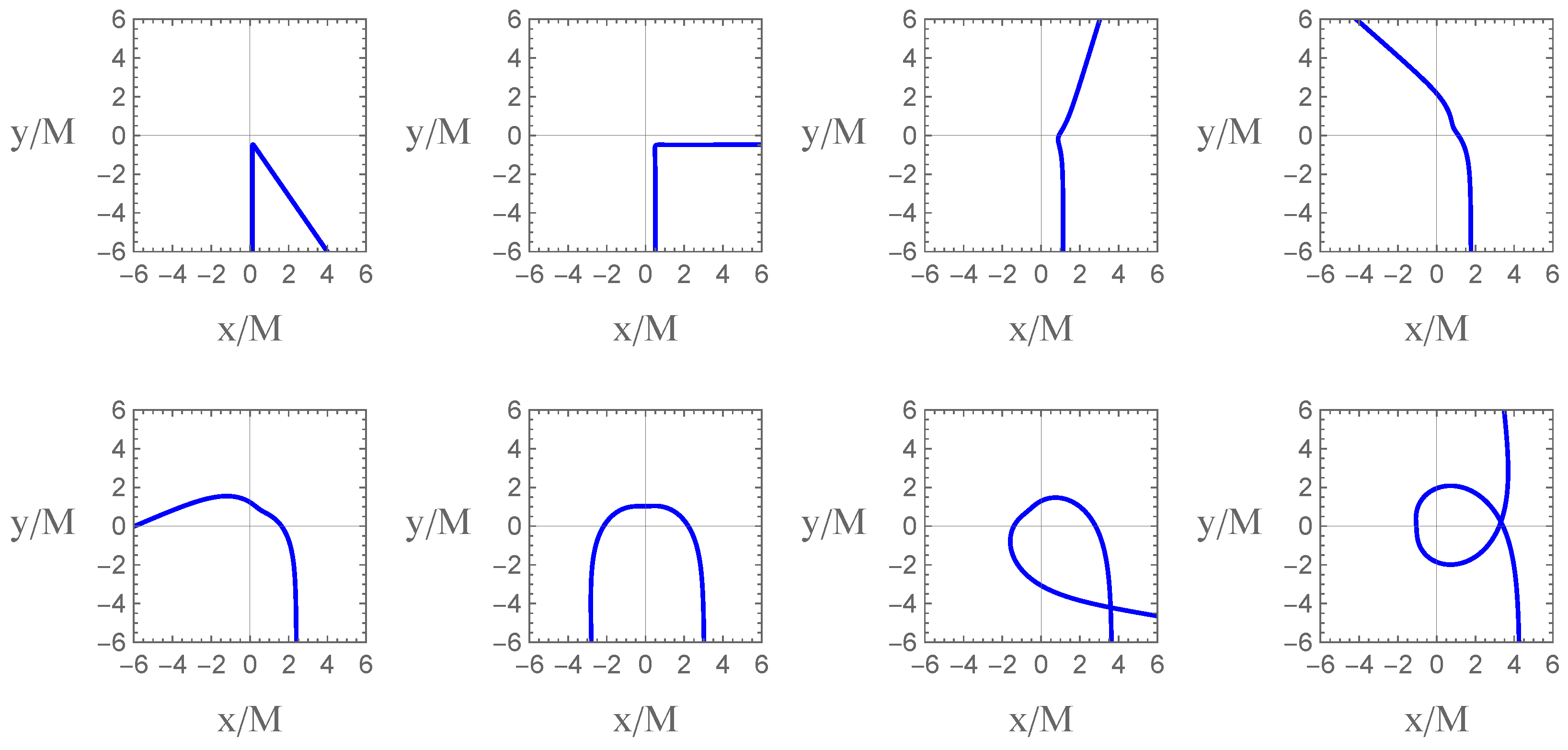
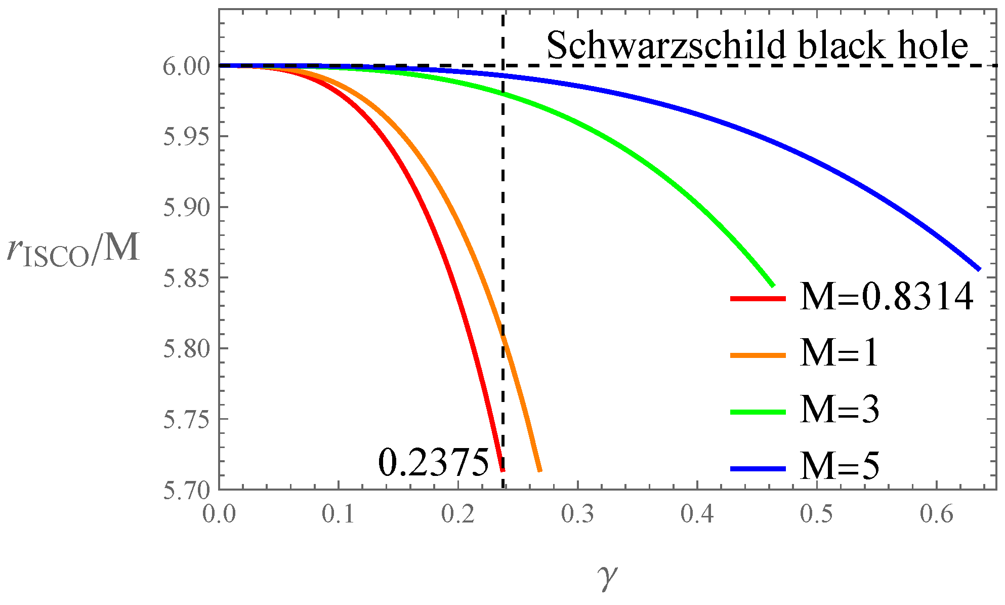
2. Null Geodesics in the Quantum-Corrected Spacetime

For a static, spherically symmetric quantum-corrected black hole (QBH) solution, the line element is given by [34]

$$d{s}^2=-f(r)d{t}^2+f{(r)}^{-1}d{r}^2+r^2(d{\theta }^2+{sin}^2\theta d{\varphi }^2),$$

(1)

with

$$f(r)=1-{\displaystyle \frac{2M}{r}}+{\displaystyle \frac{\beta M^2}{r^4}},\beta =16\sqrt{3}\pi {\gamma }^3{\ell }_p^2,$$

(2)

where ${\ell }_p=\sqrt{{\displaystyle \frac{ћG}{c^3}}}$ is the Planck length and $\gamma$ is the Barbero–Immirzi parameter (determined to be $0.2375$ in [38,39]). We adopt natural units ($c=G=ћ=1$), resulting in $\beta =16\sqrt{3}\pi {\gamma }^3\approx 1.16633$. To ensure that $f(r)=0$ has real roots, M must have a minimum value of $M_{\min }={\displaystyle \frac{16\gamma \sqrt{\pi \gamma }}{3\sqrt{3}}}\approx 0.8314$. By solving $f(r)=0$, we find that the event horizon radius $r_{\pm }$ of this QBH is

$$\begin{array}{cc}\hfill r_{\pm }& ={\displaystyle \frac{1}{6}}(3M+\sqrt{3}\sqrt{{\left(6\sigma \right)}^{{\displaystyle \frac{1}{3}}}+3M^2+{\displaystyle \frac{2\times 6^{\frac{2}{3}}{M}^2\beta }{{\left(\sigma \right)}^{\frac{1}{3}}}}})\hfill \\ \hfill & \pm {\displaystyle \frac{1}{6}}\sqrt{3}\sqrt{6M^2-{\displaystyle \frac{2\times 6^{\frac{2}{3}}{M}^2\beta }{{\left(\sigma \right)}^{\frac{1}{3}}}}-{\left(6\sigma \right)}^{{\displaystyle \frac{1}{3}}}+{\displaystyle \frac{6\sqrt{3}{M}^3}{\sqrt{{\left(6\sigma \right)}^{\frac{1}{3}}+3M^2+\frac{2 \times 6^{\frac{2}{3}}{M}^2\beta }{{\left(\sigma \right)}^{\frac{1}{3}}}}}}},\hfill \end{array}$$

(3)

where $\sigma =9M^4\beta +\sqrt{3}\sqrt{M^6\left(27M^2-16\beta \right){\beta }^2}$. Figure 2 illustrates the variation of $r_{\pm }$ with $\gamma$ for different values of M. A specific value of $\gamma$ can be observed where $r_{+}$ and $r_{-}$ converge, beyond which no horizon exists. For $M=0.8314$, this critical value of $\gamma$ is $0.2375$ ($\beta =1.16633$). Additionally, LQG corrections result in $r_{+}$ and $r_{-}$ always being smaller than the Schwarzschild black hole’s horizon radius. In the subsequent calculations, we set $M=1$.

Next, we analyze the motion of test particles within the QBH spacetime. The Lagrangian for these test particles is expressed as

$$\mathcal{L}={\displaystyle \frac{1}{2}}{g}_{\mu \nu }{\dot{x}}^{\mu }{\dot{x}}^{\nu }={\displaystyle \frac{1}{2}}\left(-f\left(r\right){\dot{t}}^2+{\displaystyle \frac{1}{f\left(r\right)}}{\dot{r}}^2+r^2{\dot{\theta }}^2+r^2{sin}^2\theta {\dot{\varphi }}^2\right),$$

(4)

where ${\dot{x}}^{\mu }={\displaystyle \frac{d{x}^{\mu }}{d\lambda }}$. For photons, $\lambda$ represents the affine parameter, while for time-like particles, $\lambda$ corresponds to the proper time $\tau$. The presence of two killing vector fields, ${\displaystyle \frac{\partial }{\partial t}}$ and ${\displaystyle \frac{\partial }{\partial \varphi }}$, in a static, spherically symmetric spacetime results in two corresponding conserved quantities for the test particles,

$$E=-{\displaystyle \frac{\partial \mathcal{L}}{\partial \dot{t}}}=f\left(r\right)\dot{t},$$

(5)

and

$$L={\displaystyle \frac{\partial \mathcal{L}}{\partial \dot{\varphi }}}=r^2\dot{\varphi },$$

(6)

where E represents the energy of the test particle, L denotes its angular momentum, and the impact parameter b is given by their ratio, $b:={\displaystyle \frac{\left|L\right|}{E}}$. Note that in Equation (6), the test particle is chosen to move on the equatorial plane, i.e., $\theta ={\displaystyle \frac{\pi }{2}}$.

For a photon, with $\mathcal{L}=0$, the equation of motion on the equatorial plane is derived by simultaneously solving Equations (4)–(6), and eliminating the affine parameter, resulting in

$$G\left(u,b\right):={\left({\displaystyle \frac{du}{d\varphi }}\right)}^2={\displaystyle \frac{1}{b^2}}-u^{2}f\left({\displaystyle \frac{1}{u}}\right),$$

(7)

where $u={\displaystyle \frac{1}{r}}$. Circular orbital motion satisfies $G\left(u,b\right)={\partial }_{u}G\left(u,b\right)=0$. Solving this yields the photon sphere radius $r_{ph}$ and the corresponding critical impact parameter $b_c$ as

$$\begin{array}{cc}\hfill r_{ph}=& {\displaystyle \frac{3M}{4}}+{\displaystyle \frac{1}{2}}\sqrt{{\displaystyle \frac{9M^2}{4}}+{\displaystyle \frac{4M{\beta }^{2/3}}{\eta }}+M{\beta }^{1/3}\eta }\hfill \\ & +{\displaystyle \frac{1}{2}}\sqrt{{\displaystyle \frac{9M^2}{2}}-{\displaystyle \frac{4M{\beta }^{2/3}}{\eta }}-{\beta }^{1/3}\eta M+{\displaystyle \frac{27M^3}{4\sqrt{\frac{9M^2}{4}+\frac{4M{\beta }^{2/3}}{\eta }+{\beta }^{1/3}\eta M}}}},\hfill \end{array}$$

(8)

$$b_c={\displaystyle \frac{r_{ph}}{\sqrt{f\left(r_{ph}\right)}}},$$

(9)

where $\eta ={\left({\displaystyle \frac{27M-\sqrt{729M^2-256\beta }}{2}}\right)}^{1/3}$. The periastron radius $r_{pe}$ of the photon’s motion satisfies $G({\displaystyle \frac{1}{r_{pe}}},b)=0$. In Figure 3, we have plotted the variation of $r_{pe}$ with b. It is evident that for $b<b_c$, $r_{pe}$ is always less than $r_{-}$ and undergoes a sudden change at $b=b_c$. The inset shows the trajectory formed by these periastron on the equatorial plane.

Figure 4, which illustrates the $G(u,b)$ function, indicates that photons with $b⩾b_c$ in the QBH spacetime move similarly to those in the Schwarzschild spacetime. However, photons with $b<b_c$ sequentially enter the outer and inner horizons, and then reach their periastron. As seen in Figure 3, these periastrons are all located within the inner horizon. According to [37], the radius of the inner horizon $r_{-}$ is a characteristic radius where the spacetime becomes highly quantized. As mentioned earlier, photons travel through this highly quantum region, disappear at their periastron, and then reappear from a white hole (corresponding to WH in Figure 1), continuing their motion along a symmetrical trajectory and eventually moving to infinity. When static observers at infinity (corresponding to q in Figure 1) receive these photons, they can obtain information from the companion black hole spacetime (corresponding to ${\mathrm{A}}^{\prime }$ in Figure 1), such as images of the accretion disk. For photons with $b<b_c$, their impact parameter b remains unchanged. Therefore, the images received by observers at infinity will all be located within the circle of radius $b_c$. The accretion disk images in the next section visually illustrate this point.

For convenience in examining the images received by the observer, we treat the path from $Q_{{\mathrm{BH}}^{\prime }}$ to q as the path from q to $Q_{{\mathrm{BH}}^{\prime }}$, given the reversibility of the light path. This allows us to set the observer’s position q as the initial position of the photon, i.e., $u=0$ and $\varphi =0$. Therefore, for photons with $b<b_c$, the azimuthal angle at $r_{\mathrm{A}}$ in region $\mathrm{A}$ is

$${\varphi }_{r_{\mathrm{A}}}={\int }_0^{{\displaystyle \frac{1}{r_{\mathrm{A}}}}}{\displaystyle \frac{1}{\sqrt{G\left(u,b\right)}}}du,$$

(10)

and at $r_{{\mathrm{A}}^{\prime }}$ in region ${\mathrm{A}}^{\prime }$ is

$${\varphi }_{r_{{\mathrm{A}}^{\prime }}}=2{\int }_0^{{\displaystyle \frac{1}{r_{pe}}}}{\displaystyle \frac{1}{\sqrt{G\left(u,b\right)}}}du-{\int }_0^{{\displaystyle \frac{1}{r_{{\mathrm{A}}^{\prime }}}}}{\displaystyle \frac{1}{\sqrt{G\left(u,b\right)}}}du.$$

(11)

Thus, the position of the photon in spacetime is determined by r and ${\varphi }_r$. Using these coordinates, we have plotted the photon’s trajectory in Figure 5. In the figure, the left panel represents spacetime $\mathrm{A}$, and the right panel represents spacetime ${\mathrm{A}}^{\prime }$. Photons with $b<b_c$ (blue lines) on the left panel sequentially enter the outer horizon (boundary of the gray disk) and the inner horizon (boundary of the green disk), disappear at their periastron (spiral dashed line), and then reappear on the right panel, continuing their motion along a trajectory symmetrical to the one on the left. In fact, the trajectories on the left and right panels can be connected to form a complete trajectory, determined by the metric described in Equation (1) (as shown in Figure 6). However, according to LQG theory, this complete trajectory is truncated at the periastron, and the segments on either side are assigned different physical meanings.

3. Image of a Thin Accretion Disk Produced by a White Hole

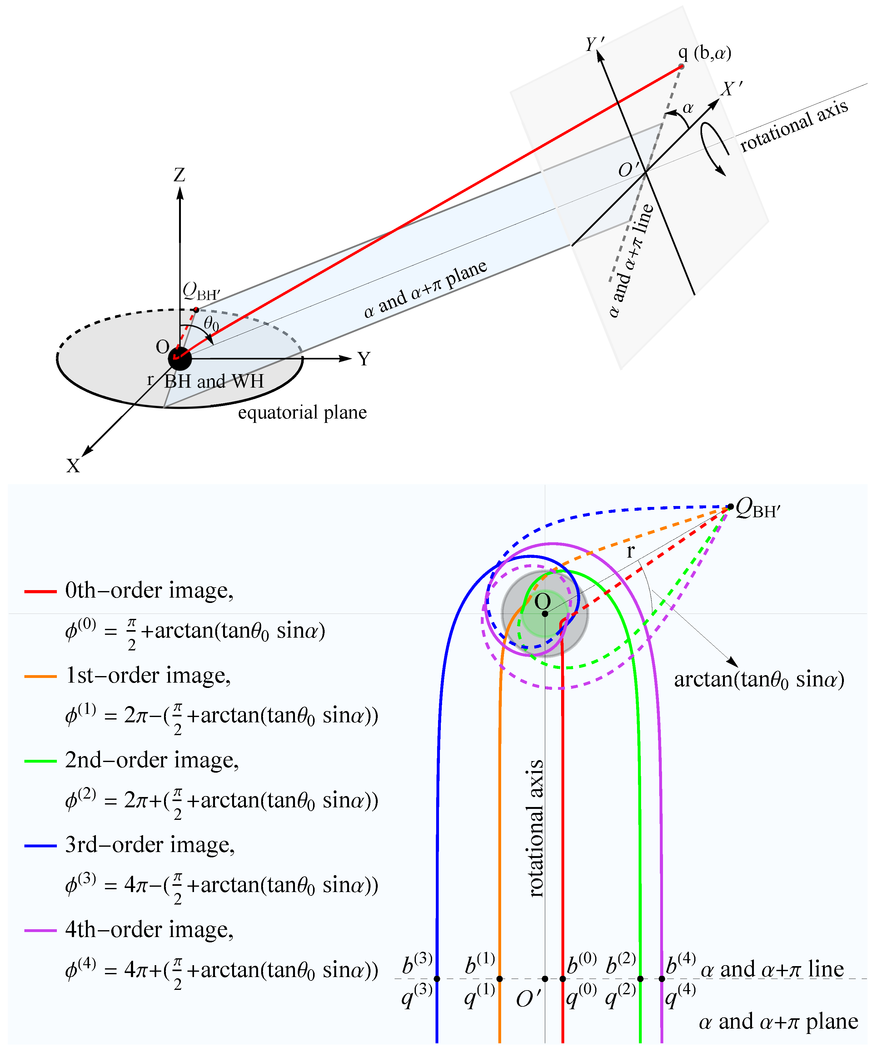
3.1. Observation Coordinate System

To derive the observed image of the accretion disk, we constructed the observational schematic diagram shown in Figure 7. In the figure, the coordinate system ${\mathrm{O}}^{\prime }{\mathrm{X}}^{\prime }{\mathrm{Y}}^{\prime }$ is positioned on the observer’s reception screen at $q\left(\infty ,{\theta }_0,0\right)$. An image point on this screen is defined by the radial coordinate b (the photon’s impact parameter) and the angular coordinate $\alpha$. The coordinate system $\mathrm{OXYZ}$ corresponds to the black hole in spacetime ${\mathrm{A}}^{\prime }$ and the white hole in spacetime $\mathrm{A}$. We represent the black hole and white hole together for the sake of their independence, which is both logical and convenient. Point $Q_{{\mathrm{BH}}^{\prime }}(r,0,\varphi )$ is located on the orbit of the accretion disk around the black hole in spacetime ${\mathrm{A}}^{\prime }$. Photons emitted from $Q_{{\mathrm{BH}}^{\prime }}$ traverse the highly quantum region of the black hole, re-emerge from a white hole in spacetime A, travel along the alpha plane, and finally reach q to form an image. This process is depicted by the red line in Figure 7, with the dashed line indicating motion in spacetime ${\mathrm{A}}^{\prime }$ and the solid line representing motion in spacetime A. Owing to the intense gravitational field of the black hole, photons emitted from point $Q_{{\mathrm{BH}}^{\prime }}$ with varying impact parameters b can reach point q along the alpha plane. This scenario is illustrated in the lower part of Figure 7. The images produced by photons can be categorized into $n (n\in \mathbb{N})$ orders based on the magnitude of the $\varphi$ angle they traverse, with the corresponding $\varphi$ angles for these n orders given by

$${\varphi }^{(n)}({\theta }_0,\alpha )=\left\{\begin{array}{cc}{\displaystyle \frac{n}{2}}2\pi +{\left(-1\right)}^n\left[{\displaystyle \frac{\pi }{2}}+\mathrm{arc}tan\left(tan{\theta }_{0}sin\alpha \right)\right]\hfill & , \mathrm{when} n \mathrm{is} \mathrm{even},\hfill \\ {\displaystyle \frac{n+1}{2}}2\pi +{\left(-1\right)}^n\left[{\displaystyle \frac{\pi }{2}}+\mathrm{arc}tan\left(tan{\theta }_{0}sin\alpha \right)\right]\hfill & , \mathrm{when} n \mathrm{is} \mathrm{odd}.\hfill \end{array}\right.$$

(12)

Substituting ${\varphi }^{(n)}({\theta }_0,\alpha )$ into Equation (11) yields $b^{(n)}$. Together, $b^{(n)}$ and $\alpha$ define an image point on the observer’s reception screen.

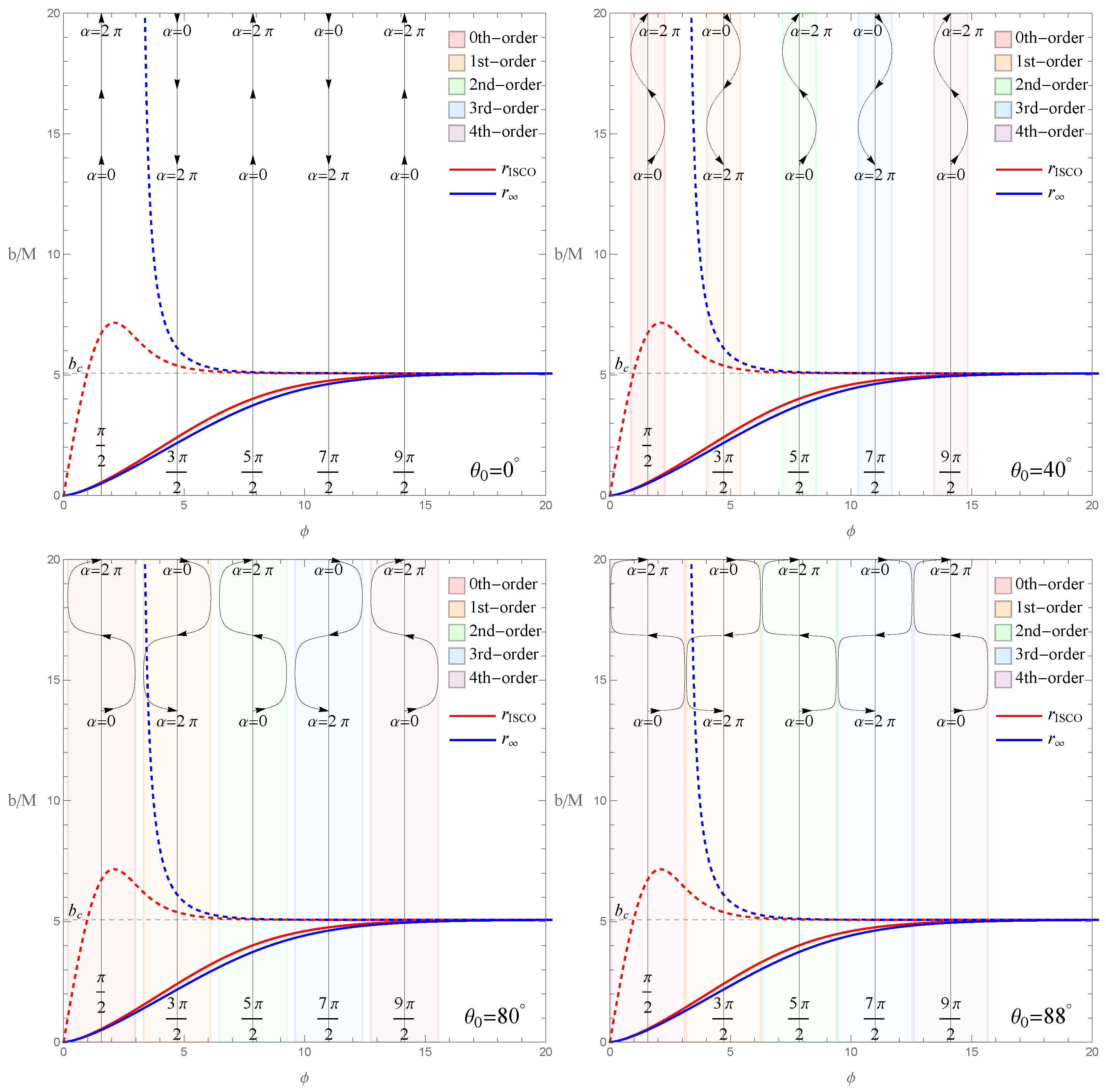
3.2. Image of a Thin Accretion Disk

Geometrically, the accretion disk is a flat, wide, ring-like structure, theoretically composed of matter accumulated between the innermost stable circular orbit and an outer circular orbit. For simplicity, we assume the accretion disk extends between $r=r_{\mathrm{ISCO}}$ and $r=r_{\infty }\equiv \infty$. $r_{\mathrm{ISCO}}$ represents the innermost stable circular orbit (ISCO) for timelike particles, which satisfies the condition ${\left.{\dot{r}}^2\right|}_{r_{\mathrm{ISCO}}}={\left.\left({\partial }_r{\dot{r}}^2\right)\right|}_{r_{\mathrm{ISCO}}}={\left.\left({\partial }_{r,r}{\dot{r}}^2\right)\right|}_{r_{\mathrm{ISCO}}}=0$, where ${\dot{r}}^2\equiv {\left({\partial }_{\tau }r\right)}^2={\displaystyle \frac{1}{b^2}}-{\displaystyle \frac{f\left(r\right)}{r^2}}-{\displaystyle \frac{f\left(r\right)}{L^2}}$. Figure 8 illustrates the variation of $r_{ISCO}$ with $\gamma$ for different values of M. At $\gamma =0$, $r_{ISCO}=6$, corresponding to the Schwarzschild black hole. As $\gamma$ increases, $r_{ISCO}$ decreases, while as M increases, $r_{ISCO}$ increases. Therefore, LQG corrections always reduce $r_{ISCO}$.

We trace a photon with $b<b_c$, which is emitted from point q, enters the white hole, re-emerges from the black hole (considering the reverse process for convenience), and finally reaches the accretion disk at radius r. During this process, the photon undergoes a change in the $\varphi$ angle, denoted as $\varphi (b,r)$. In fact, it corresponds exactly to $\varphi$ in Equation (11). While we could plot the function $\varphi (b,r)$, for the following discussion, we have instead plotted $b(\varphi ,r)$ in Figure 9.

In the diagram, the S-shaped curve with an arrow represents the function $\alpha (\varphi )$, which is the inverse of $\varphi (\alpha )$, as defined in Equation (12). The red solid line corresponds to the circular orbit at $r_{\mathrm{ISCO}}$, while the blue solid line corresponds to the circular orbit at $r_{\infty }$. The dashed line illustrates the scenario where the photon does not traverse the high quantum region or, equivalently, the situation where an observer at infinity in spacetime ${\mathrm{A}}^{\prime }$ observes the black hole’s accretion disk, corresponding to the traditional accretion disk image. The five colored strip regions, as determined by Equation (12), represent the range of $\varphi$ angles for different orders.

Using Figure 9: Select an angle ${\theta }_0$ and an order n, then identify a point on the corresponding S-shaped curve that matches a specific value of $\alpha$, with $\alpha$ increasing from 0 to $2\pi$ in the direction indicated by the arrow. Draw a vertical line from this point, perpendicular to the $\varphi$-axis, to determine the value of $\varphi$. Then, calculate the b value at the intersection of this vertical line with either the red or blue curve. After completing these steps, the values of $\alpha$ and b are obtained, determining the position of the image point on the observer’s reception screen formed by photons emitted from particles on the accretion disk orbit at radii $r_{\mathrm{ISCO}}$ or $r_{\infty }$. By repeating this process for each $\alpha$ value from 0 to $2\pi$, the nth order image of the accretion disk with radius r is obtained.

From Figure 9, the following properties of the accretion disk images produced by the white hole can be observed:

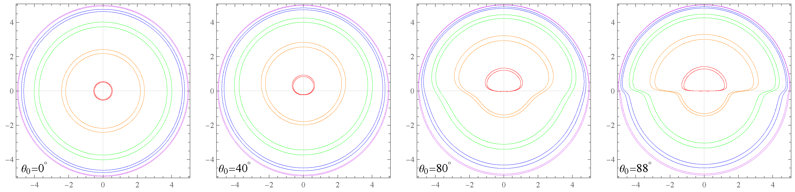
(a)

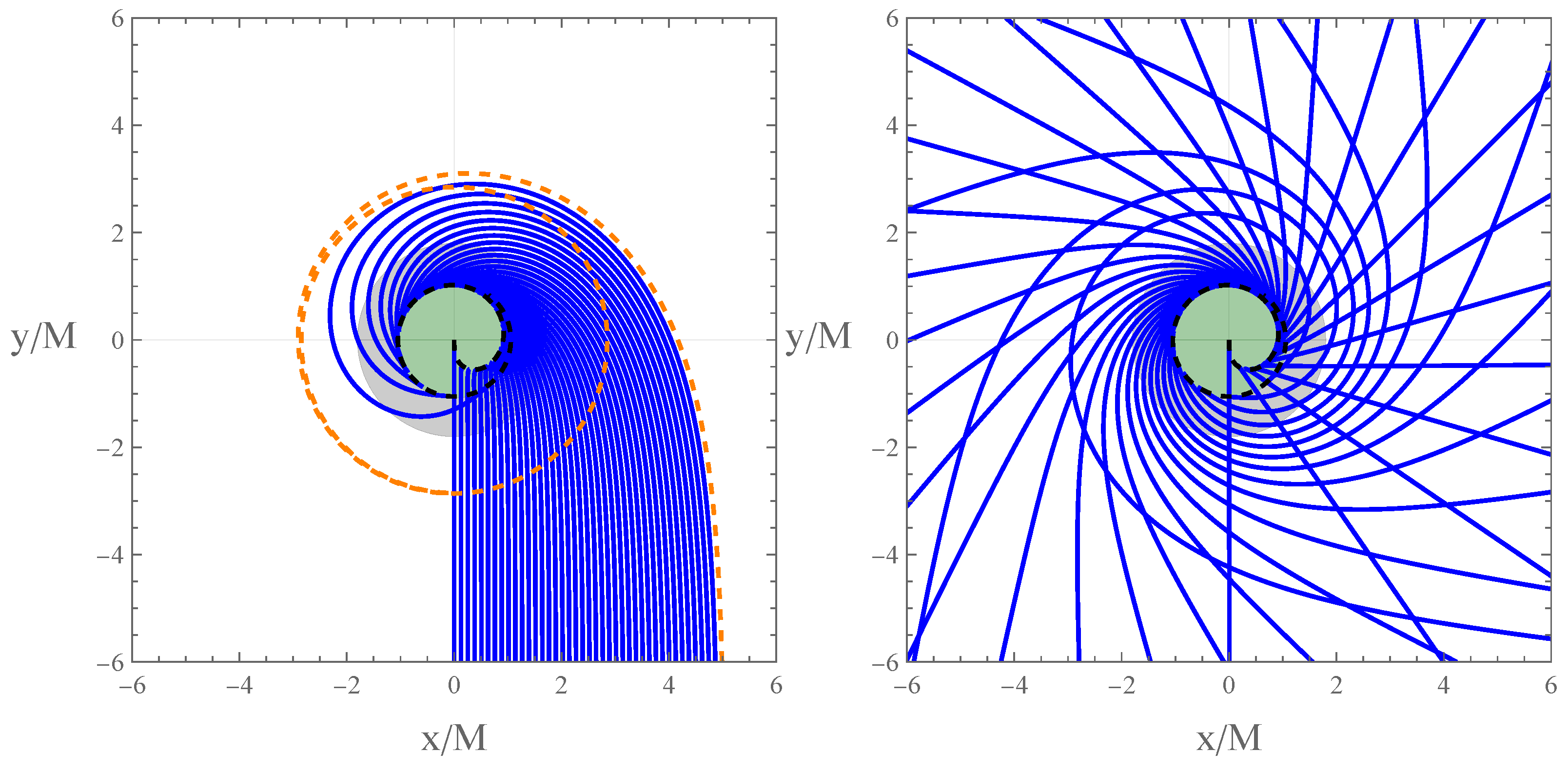
All accretion disk images are confined within a circle of radius $b_c$;

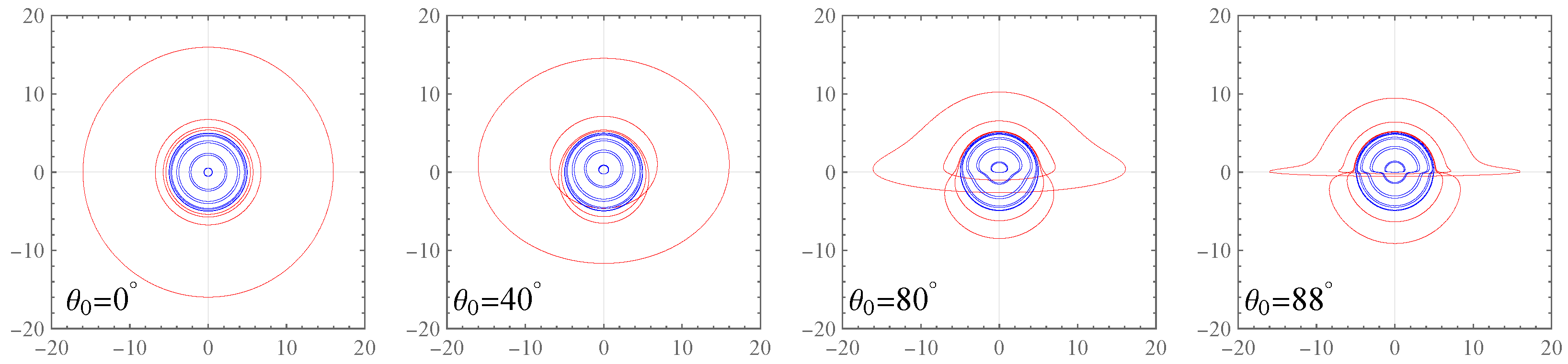
(b)

Images corresponding to larger orbital radii have smaller b values and appear on the inner side of the image, which is the opposite of what occurs with traditional accretion disk images;

(c)

The 2nd-order image of the accretion disk is the widest, whereas the 0th-order image is very narrow. In contrast, in traditional accretion disk images, the 0th-order is the widest. Additionally, compared to traditional accretion disk images, even the widest image produced by the white hole remains relatively narrow. It is important to note that the blue curve plotted corresponds to the circular orbit at $r_{\infty }$. Since the actual outermost circular orbit of the accretion disk has a finite radius, the disk image will be even narrower;

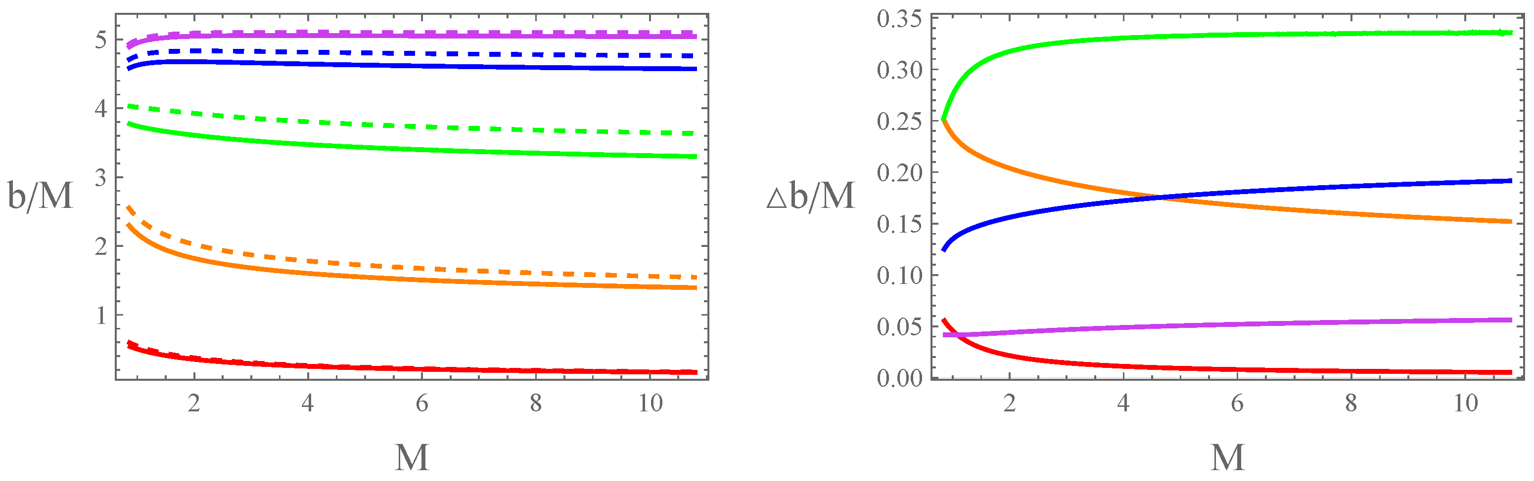
(d)

As ${\theta }_0$ increases, the value of b increases in $\alpha \in \left(0,\pi \right)$, while it decreases in $\alpha \in \left(\pi ,2\pi \right)$. This causes the upper part of the accretion disk image to enlarge and the lower part to shrink, resulting in a shell-like shape. This contrasts sharply with traditional accretion disk images beyond the 1st-order. Additionally, the variation in accretion disk image width with respect to $\alpha$ differs from that of traditional accretion disks. For instance, in the 1st-order image, the traditional accretion disk is widest at $\alpha ={\displaystyle \frac{3\pi }{2}}$, whereas the accretion disk image produced by the white hole is widest at $\alpha ={\displaystyle \frac{\pi }{2}}$;

(e)

Other features of the accretion disk images are generally consistent with those of traditional accretion disk images, including the circular nature of the 0th-order image and the symmetry of the images about the $y$-axis.

Figure 10 illustrates the accretion disk images, clearly demonstrating the characteristics described above. For ${\theta }_0=0^{\circ }$, the corresponding values of $(b_{min}/M,b_{max}/M)$ for $n=0, 1, 2, 3$, and 4 are $(0.50389,0.547009)$, $(2.17901,2.41511)$, $(3.74008,4.01542)$, $(4.62536,4.7603)$, and $(4.94967,4.99131)$, respectively. Additionally, for better comparison, Figure 11 combines the traditional black hole accretion disk images (represented by the dashed lines in Figure 9) with the accretion disk images produced by the white hole. Note that the red dashed line corresponding to $r=r_{\infty }$ was adjusted to $r=15M$ to enable the plotting of the 0th-order image, which would otherwise be impossible.

Figure 12 illustrates the variation in edge positions and widths of the first five-order images as a function of M when ${\theta }_0=0^{\circ }$. It is evident that the 2nd-order image is the widest, while the 0th-order image is the narrowest in most cases. As the order n increases, the positions of these images cluster around $b_c$. Additionally, it can be observed that as M approaches infinity, both the position and width converge to a fixed limiting value, a result already demonstrated in [37].

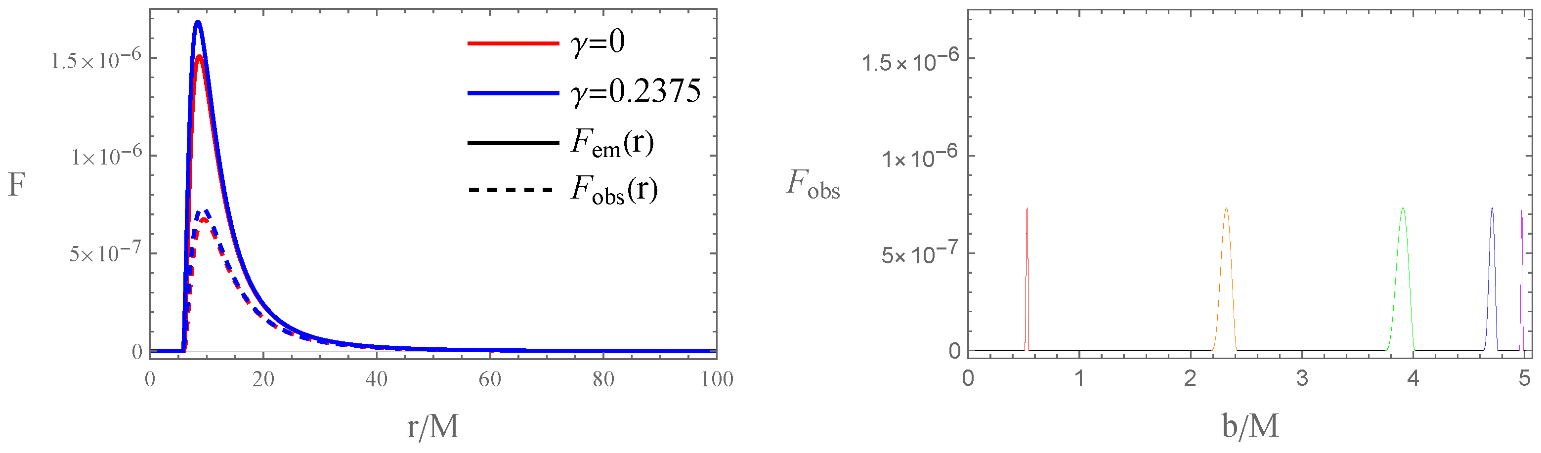
3.3. Light Intensity Distribution on Accretion Disk

We used the Novikov–Thorne model to analyze the luminous images of accretion disks. As described in [40], the radiation flux of photons emitted by particles on the accretion disk at a radius r is given by

$$F_{em}\left(r\right)=-{\displaystyle \frac{\mathcal{M}{\Omega }^{\prime }}{4\pi \sqrt{-g}{\left(E-\Omega L\right)}^2}}{\int }_{r_{isco}}^r\left(E-\Omega L\right)L^{\prime }dr,$$

(13)

where $\mathcal{M}$ denotes the black hole’s accretion rate, g represents the determinant of the metric, and E, L, and $\Omega$ stand for the energy, angular momentum, and angular velocity of the particles in the accretion disk, respectively.

Due to the differences in gravitational fields between the disk and the observer, as well as their relative motion, a frequency shift occurs. Consequently, the radiation flux observed is [41,42,43]

$$F_{obs}(r)={\displaystyle \frac{F_{em}\left(r\right)}{{\left(1+z\right)}^4}},$$

(14)

where z is redshift factor. From [44], we obtain

$$F_{obs}(r)={\displaystyle \frac{-\frac{\mathcal{M}{\Omega }^{\prime }}{4\pi \sqrt{-g}{\left(E - \Omega L\right)}^2}{\int }_{r_{isco}}^r\left(E-\Omega L\right)L^{\prime }dr}{{\left(\frac{1 + \Omega bsin\theta cos\alpha }{\sqrt{-g_{tt} - g_{\varphi \varphi }{\Omega }^2}}\right)}^4}},$$

(15)

where

$$\Omega =\pm \sqrt{-{\displaystyle \frac{g_{tt}^{\prime }}{g_{\varphi \varphi }^{\prime }}}},$$

(16)

$$E=-g_{t\mu }{U}^{\mu }={\displaystyle \frac{-g_{tt}}{\sqrt{-g_{tt}-g_{\varphi \varphi }{\Omega }^2}}},$$

(17)

$$L=g_{\varphi \mu }{U}^{\mu }={\displaystyle \frac{g_{\varphi \varphi }\Omega }{\sqrt{-g_{tt}-g_{\varphi \varphi }{\Omega }^2}}}.$$

(18)

Another crucial physical property of the accretion disk is its radiation efficiency, which quantifies the energy released as radiation during matter accretion onto a black hole. Assuming all photons emitted by the particles can escape to infinity, the radiation efficiency is expressed as

$$ϵ={\displaystyle \frac{E_{\infty }-E_{ISCO}}{E_{\infty }}},$$

(19)

where $E_{\infty }$ is the energy of the particle at infinity, and $E_{ISCO}$ is the energy at the ISCO. From Equation (17), since $E_{\infty }=1$, we have

$$ϵ=1-E_{ISCO}.$$

(20)

Figure 13 illustrates the variation of $ϵ$ with $\gamma$ for different values of M. When $\gamma =0$, $ϵ=0.0572$, it corresponds to the radiation efficiency of the Schwarzschild black hole. As $\gamma$ increases, $ϵ$ rises, while as M increases, $ϵ$ decreases. This suggests that LQG corrections convert more particle energy into radiation, enhancing the brightness of the accretion disk, as shown in Figure 14.

Figure 14 illustrates the variation of $F_{em}(r)$ and $F_{obs}(r)$, with respect to r (left) and the variation of $F_{obs}$ with b (right) when ${\theta }_0=0^{\circ }$. Due to redshift, $F_{obs}(r)$ is significantly smaller than $F_{em}(r)$, while LQG corrections enhance the brightness of the accretion disk. Additionally, $F_{obs}(r)$ is compressed within each order’s image, with each order containing the full information of $F_{obs}(r)$, but at varying levels of compression.

Figure 15 presents the luminous images of accretion disks. Similar to traditional accretion disk images, the light intensity distribution is asymmetrical about the y-axis due to gravitational redshift and Doppler effects. As ${\theta }_0$ increases, the left side of the image progressively brightens, while the right side darkens. Unlike traditional accretion disk images, in which the inner region is illuminated by particles on orbits with smaller radii, here, the inner region of each order’s image is illuminated by particles on orbits with larger radii, while the outer region is illuminated by particles on orbits with smaller radii. Consequently, a broader dark area forms on the inner side and a narrower dark area on the outer side, as $F_{obs}(r)$ in Figure 14 flattens more at $r<r_m$ than at $r>r_m$, where $r_m$ is the radius at which $F_{obs}(r)$ reaches its maximum. A close examination of Figure 15 reveals this phenomenon, which becomes even more apparent in Figure 3 of [37], as the emission model in [37] exhibits a discontinuity at $r_m$. In that figure, the traditional black hole image shows a darker outer region, while the image produced by a white hole displays a darker inner region.

4. Summary

In this paper, we obtained accretion disk images produced by a white hole from various observational angles and analyzed their properties. In Section 2, we studied the geodesics of photons with $b<b_c$ in a quantum-corrected spacetime. The results indicate that photons do not vanish at the black hole’s event horizon; rather, they continue their motion, sequentially crossing the outer and inner horizons, reaching periastron, and eventually re-emerging from a white hole. In Section 3, we established an observation system and generated accretion disk images produced by the white hole, analyzing their light intensity distribution using the Novikov–Thorne model. The results indicate that most properties of accretion disk images produced by the white hole are opposite to those of traditional accretion disk images. The images produced by the white hole are confined within a circle of radius $b_c$. As the order n increases, these images gradually transform into circles with no width, clustering near $b_c$. The images corresponding to orbits with larger radii are located on the outer edge of each order’s accretion disk image, while those with smaller radii appear on the inner side. This leads to a broader dark region on the inner side of the bright accretion disk image compared to the outer side. Compared to the Schwarzschild black hole, LQG corrections reduce the ISCO radius, enhancing the radiation efficiency of the accretion disk and increasing its brightness. As the observation angle ${\theta }_0$ increases from 0, the accretion disk image produced by the white hole transforms from a ring to a shell-like shape, with the upper half expanding and the lower half contracting. Additionally, the 2nd-order accretion disk image has the greatest width, while the 0th-order image has the narrowest, though both are much narrower than the first two orders of traditional accretion disk images. Similar to traditional accretion disk images, these images are all symmetric about the y-axis.

Our work complements and extends the research of Zhang et al. [37]. While this idea has many limitations, it qualitatively represents a bold and intriguing attempt. Quantum gravity theories hold significant promise in resolving singularity issues, although the observable effects are often subtle. However, the additional accretion disk images produced by white holes are notably distinct. These images could aid in validating quantum gravity theories and distinguishing between different quantum gravity models.

References

- Penrose, R. Gravitational collapse and space-time singularities. Phys. Rev. Lett. 1965, 14, 57. [Google Scholar] [CrossRef]
- Hawking, S.; Penrose, R. Proceedings the royal-of-society. Proc. R. Soc. Lond. A 1970, 1970. [Google Scholar]
- Hawking, S.W. Particle creation by black holes. Commun. Math. Phys. 1975, 43, 199–220. [Google Scholar] [CrossRef]
- Ashtekar, A.; Bojowald, M. Quantum geometry and the Schwarzschild singularity. Class. Quantum Gravity 2005, 23, 391. [Google Scholar] [CrossRef]
- Modesto, L. Loop quantum black hole. Class. Quantum Gravity 2006, 23, 5587. [Google Scholar] [CrossRef]
- Cartin, D.; Khanna, G. Wave functions for the Schwarzschild black hole interior. Phys. Rev. D 2006, 73, 104009. [Google Scholar] [CrossRef]
- Boehmer, C.G.; Vandersloot, K. Loop quantum dynamics of the Schwarzschild interior. Phys. Rev. D 2007, 76, 104030. [Google Scholar] [CrossRef]
- Chiou, D.W. Phenomenological loop quantum geometry of the Schwarzschild black hole. Phys. Rev. D 2008, 78, 064040. [Google Scholar] [CrossRef]
- Campiglia, M.; Gambini, R.; Pullin, J. Loop quantization of spherically symmetric midi-superspaces: The interior problem. AIP Conf. Proc. 2007, 24, 3649–3672. [Google Scholar] [CrossRef]
- Akiyama, K.; Alberdi, A.; Alef, W.; Asada, K.; Azulay, R.; Baczko, A.K.; Ball, D.; Baloković, M.; Barrett, J.; Bintley, D.; et al. First M87 event horizon telescope results. VI. The shadow and mass of the central black hole. Astrophys. J. Lett. 2019, 875, L6. [Google Scholar]
- Giesel, K.; Thiemann, T. Algebraic quantum gravity (AQG): IV. Reduced phase space quantization of loop quantum gravity. Class. Quantum Gravity 2010, 27, 175009. [Google Scholar] [CrossRef]
- Gambini, R.; Pullin, J. Loop quantization of the Schwarzschild black hole. Phys. Rev. Lett. 2013, 110, 211301. [Google Scholar] [CrossRef]
- Bianchi, E.; Dona, P.; Speziale, S. Polyhedra in loop quantum gravity. Phys. Rev. D 2011, 83, 044035. [Google Scholar] [CrossRef]
- Gambini, R.; Olmedo, J.; Pullin, J. Quantum black holes in loop quantum gravity. Class. Quantum Gravity 2014, 31, 095009. [Google Scholar] [CrossRef]
- Hooft, G. How quantization of gravity leads to a discrete space-time. J. Phys. Conf. Ser. 2016, 701, 012014. [Google Scholar] [CrossRef]
- Ashtekar, A.; Bianchi, E. A short review of loop quantum gravity. Rep. Prog. Phys. 2021, 84, 042001. [Google Scholar] [CrossRef]
- McCabe, G. Loop Quantum Gravity and Discrete Space-Time. PhilSci Archive. 2018. Available online: http://philsci-archive.pitt.edu/14959/ (accessed on 8 October 2024).
- Wang, C.H.T.; Rodrigues, D.P. Closing the gaps in quantum space and time: Conformally augmented gauge structure of gravitation. Phys. Rev. D 2018, 98, 124041. [Google Scholar] [CrossRef]
- Kelly, J.G.; Santacruz, R.; Wilson-Ewing, E. Black hole collapse and bounce in effective loop quantum gravity. Class. Quantum Gravity 2020, 38, 04LT01. [Google Scholar] [CrossRef]
- Perez, A. Black holes in loop quantum gravity. Rep. Prog. Phys. 2017, 80, 126901. [Google Scholar] [CrossRef]
- Bouhmadi-López, M.; Brahma, S.; Chen, C.Y.; Chen, P.; Yeom, D.h. A consistent model of non-singular Schwarzschild black hole in loop quantum gravity and its quasinormal modes. J. Cosmol. Astropart. Phys. 2020, 2020, 066. [Google Scholar] [CrossRef]
- Ashtekar, A.; Olmedo, J.; Singh, P. Regular black holes from loop quantum gravity. In Regular Black Holes; Springer: Singapore, 2023; pp. 235–282. [Google Scholar]
- Olmedo, J.; Saini, S.; Singh, P. From black holes to white holes: A quantum gravitational, symmetric bounce. Class. Quantum Gravity 2017, 34, 225011. [Google Scholar] [CrossRef]
- Abedi, J.; Arfaei, H. Obstruction of black hole singularity by quantum field theory effects. J. High Energy Phys. 2016, 2016, 135. [Google Scholar] [CrossRef]
- Oppenheimer, J.R.; Snyder, H. On continued gravitational contraction. Phys. Rev. 1939, 56, 455. [Google Scholar] [CrossRef]
- Bojowald, M.; Goswami, R.; Maartens, R.; Singh, P. Black hole mass threshold from nonsingular quantum gravitational collapse. Phys. Rev. Lett. 2005, 95, 091302. [Google Scholar] [CrossRef] [PubMed]
- Bojowald, M.; Reyes, J.D.; Tibrewala, R. Nonmarginal Lemaitre-Tolman-Bondi-like models with inverse triad corrections from loop quantum gravity. Phys. Rev. D 2009, 80, 084002. [Google Scholar] [CrossRef]
- Marto, J.; Tavakoli, Y.; Moniz, P.V. Improved dynamics and gravitational collapse of tachyon field coupled with a barotropic fluid. Int. J. Mod. Phys. D 2015, 24, 1550025. [Google Scholar] [CrossRef]
- Achour, J.B.; Brahma, S.; Uzan, J.P. Bouncing compact objects. Part I. Quantum extension of the Oppenheimer-Snyder collapse. J. Cosmol. Astropart. Phys. 2020, 2020, 041. [Google Scholar] [CrossRef]
- Achour, J.B.; Brahma, S.; Mukohyama, S.; Uzan, J.P. Towards consistent black-to-white hole bounces from matter collapse. J. Cosmol. Astropart. Phys. 2020, 2020, 020. [Google Scholar] [CrossRef]
- Münch, J. Effective quantum dust collapse via surface matching. Class. Quantum Gravity 2021, 38, 175015. [Google Scholar] [CrossRef]
- Münch, J. Causal structure of a recent loop quantum gravity black hole collapse model. Phys. Rev. D 2021, 104, 046019. [Google Scholar] [CrossRef]
- Husain, V.; Kelly, J.G.; Santacruz, R.; Wilson-Ewing, E. Quantum gravity of dust collapse: Shock waves from black holes. Phys. Rev. Lett. 2022, 128, 121301. [Google Scholar] [CrossRef] [PubMed]
- Lewandowski, J.; Ma, Y.; Yang, J.; Zhang, C. Quantum oppenheimer-snyder and swiss cheese models. Phys. Rev. Lett. 2023, 130, 101501. [Google Scholar] [CrossRef] [PubMed]
- Ashtekar, A.; Olmedo, J.; Singh, P. Quantum transfiguration of Kruskal black holes. Phys. Rev. Lett. 2018, 121, 241301. [Google Scholar] [CrossRef] [PubMed]
- Ashtekar, A.; Olmedo, J.; Singh, P. Quantum extension of the Kruskal spacetime. Phys. Rev. D 2018, 98, 126003. [Google Scholar] [CrossRef]
- Zhang, C.; Ma, Y.; Yang, J. Black hole image encoding quantum gravity information. Phys. Rev. D 2023, 108, 104004. [Google Scholar] [CrossRef]
- Meissner, K.A. Black-hole entropy in loop quantum gravity. Class. Quantum Gravity 2004, 21, 5245. [Google Scholar] [CrossRef]
- Domagala, M.; Lewandowski, J. Black-hole entropy from quantum geometry. Class. Quantum Gravity 2004, 21, 5233. [Google Scholar] [CrossRef]
- Novikov, I.D.; Thorne, K.S. Astrophysics of black holes. In Black Holes (Les Astres Occlus); Dewitt, C., Dewitt, B.S., Eds.; Gordon and Breach: New York, NY, USA, 1973; pp. 343–450. [Google Scholar]
- Ellis, G.F.; Maartens, R.; MacCallum, M.A.H. Relativistic Cosmology; Cambridge University Press: Cambridge, UK, 2012. [Google Scholar]
- Luminet, J.P. Image of a spherical black hole with thin accretion disk. Astron. Astrophys. 1979, 75, 228–235. [Google Scholar]
- Huang, Y.X.; Guo, S.; Cui, Y.H.; Jiang, Q.Q.; Lin, K. Influence of accretion disk on the optical appearance of the Kazakov-Solodukhin black hole. Phys. Rev. D 2023, 107, 123009. [Google Scholar] [CrossRef]
- You, L.; Wang, R.b.; Ma, S.J.; Deng, J.B.; Hu, X.R. Optical properties of Euler-Heisenberg black hole in the Cold Dark Matter Halo. arXiv 2024, arXiv:2403.12840. [Google Scholar]
Disclaimer/Publisher’s Note: The statements, opinions and data contained in all publications are solely those of the individual author(s) and contributor(s) and not of MDPI and/or the editor(s). MDPI and/or the editor(s) disclaim responsibility for any injury to people or property resulting from any ideas, methods, instructions or products referred to in the content. |
© 2024 by the authors. Licensee MDPI, Basel, Switzerland. This article is an open access article distributed under the terms and conditions of the Creative Commons Attribution (CC BY) license (https://creativecommons.org/licenses/by/4.0/).
Share and Cite
You, L.; Feng, Y.-H.; Wang, R.-B.; Hu, X.-R.; Deng, J.-B. Decoding Quantum Gravity Information with Black Hole Accretion Disk. Universe 2024, 10, 393. https://doi.org/10.3390/universe10100393
You L, Feng Y-H, Wang R-B, Hu X-R, Deng J-B. Decoding Quantum Gravity Information with Black Hole Accretion Disk. Universe. 2024; 10(10):393. https://doi.org/10.3390/universe10100393
Chicago/Turabian StyleYou, Lei, Yu-Hang Feng, Rui-Bo Wang, Xian-Ru Hu, and Jian-Bo Deng. 2024. "Decoding Quantum Gravity Information with Black Hole Accretion Disk" Universe 10, no. 10: 393. https://doi.org/10.3390/universe10100393
APA StyleYou, L., Feng, Y.-H., Wang, R.-B., Hu, X.-R., & Deng, J.-B. (2024). Decoding Quantum Gravity Information with Black Hole Accretion Disk. Universe, 10(10), 393. https://doi.org/10.3390/universe10100393