A New Stock Price Forecasting Method Using Active Deep Learning Approach

Abstract

Stock price prediction is a significant research field due to its importance in terms of benefits for individuals, corporations, and governments. This research explores the application of the new approach to predict the adjusted closing price of a specific corporation. A new set of features is used to enhance the possibility of giving more accurate results with fewer losses by creating a six-feature set (that includes High, Low, Volume, Open, HiLo, OpSe), rather than the traditional four-feature set (High, Low, Volume, Open). The study also investigates the effect of data size by using datasets (Apple, ExxonMobil, Tesla, Snapchat) of different sizes to boost open innovation dynamics. The effect of the business sector in terms of the loss result is also considered. Finally, the study included six deep learning models, MLP, GRU, LSTM, Bi-LSTM, CNN, and CNN-LSTM, to predict the adjusted closing price of the stocks. The six variables used (High, Low, Open, Volume, HiLo, and OpSe) are evaluated according to the model’s outcome, showing fewer losses than the original approach, which utilizes the original feature set. The results show that LSTM-based models improved using the new approach, even though all models showed a comparative result wherein no model showed better results or continuously outperformed other models. Finally, the added new features positively affected the prediction models’ performance.

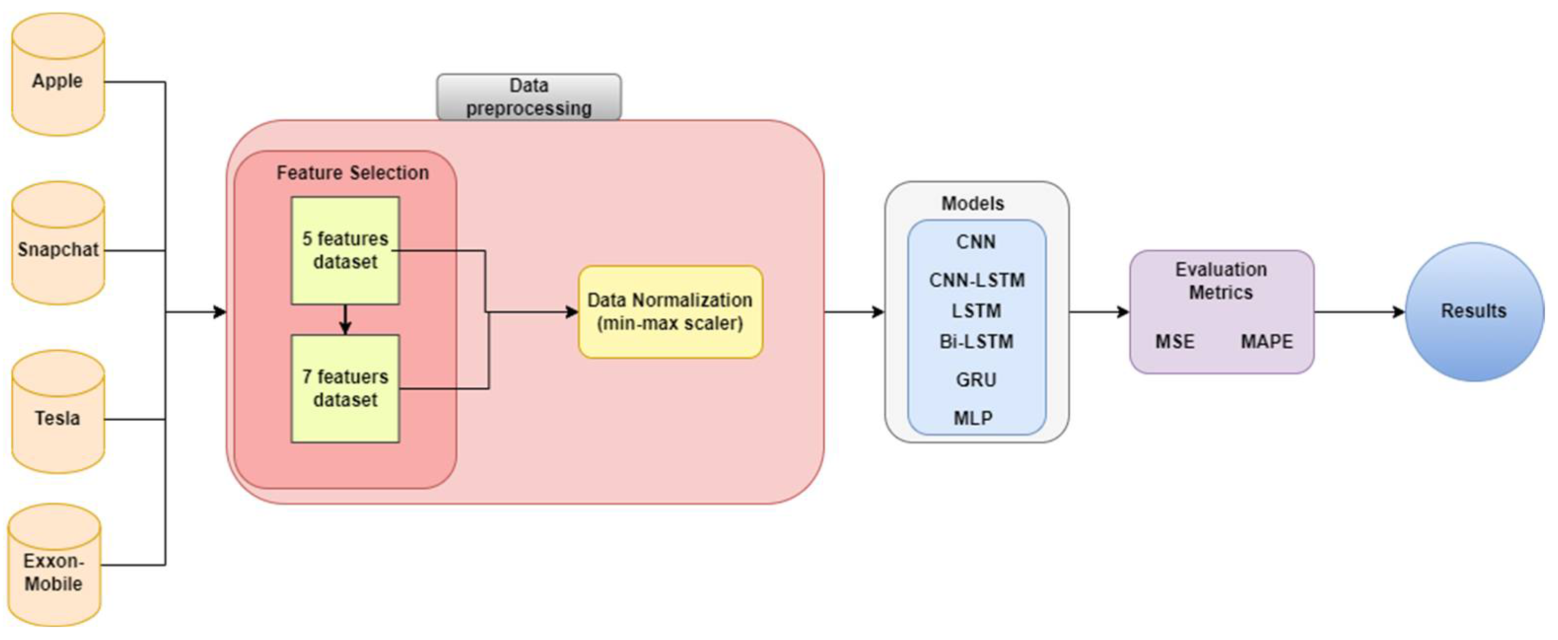
1. Introduction

Countries focus on improving and enhancing their economies to create a good standard of living by ensuring public spending. The modern economy establishes large corporations that could create enormous opportunities and keep up with rapid changes in the world economy [1,2]. The stock market is a pool of buyer and seller securities divided into the private stock exchange, open stock exchange, and mixed ownership stock exchange [3]. The private stock exchange involves exchanging shares of private companies, whereas the open stock exchange includes shares of a company listed in the public stock market. The mixed-ownership stock is in companies whose shares are only partially exchangeable in the public stock market. These stock exchanges are created in the United Kingdom, such as in the London Stock Exchange, and the United States, such as in the New York Stock Exchange (NYSE) [4,5,6,7,8,9].

Stock price forecasting is among one of the most challenging problems that financial institutions, businesses, and individual investors face [10]. Many factors impact the validity of stock price forecasts, including economics, political contexts, and investor psychology. According to the literature, because of this complexity, there is much interest in applying machine learning methods such as artificial intelligence, probabilistic reasoning, and evolutionary programming to assess large historical datasets on stock prices [11,12]. As it does not require any statistical hypotheses, an Artificial Neural Network, chiefly, a statistical and non-parametric method, is one of the most popular tools in predictive modeling among all of these computer intelligence approaches [13,14,15,16,17,18].

The stock market is the backbone of any economy; the primary purposes of any investment in the stock market are profit maximization and minimizing risk [4]; therefore, countries need to enhance their stock markets, since they are related to economic growth [19]. Investing in the stock market could lead to a quick return on investment; therefore, stock market prediction is one of the best strategies to achieve a profit. Stock market prediction is not linear, thus making it harder to predict a corporation’s stock prices in a specific market [20]. Consequently, investors and researchers have to find techniques that could lead to accurate results and higher profits [21]. Conventional machine learning models are superior to statistical models such as ARIMA [22]. On the other hand, deep learning models such as Long Short-Term Memory (LSTM) were proven to outperform machine learning models such as Support Vector Regression (SVR) [23], (KARA et al., 2011), which also showed that the deep learning model Artificial Neural Network (ANN) had been detected instead of Support Vector Machine (SVM) [24].

Forex price forecasting is similar to stock price forecasting [25,26]. An attention RNN-ARIMA (ARNN-ARIMA) model is proposed to forecast forex prices. The proposed model was evaluated using three main metrics: Root Mean Squared Error (RMSE), Mean Squared Percentage Error (MAPE), and Directional Accuracy. The proposed model has been compared with multiple models, including RNN, GRU, LSTM, and ARNN. It outperformed all other models by utilizing all metrics, subsequently achieving the lowest RMSE and MAPE with 1.65 × 10⁻³, and 23.2%, respectively, and the highest DA with 75.7%, slightly outperforming ARNN which achieved 73.5% DA [27]. An LSTM with an embedded layer model (ELSTM), and a LSTM with an Autoencoder (ALSTM), are introduced in [28]. The proposed model compared multiple metrics to evaluate its performance compared with multiple models. In addition to the two datasets, the first experiment on the first dataset, using ALSTM and ELSTM, revealed a good performance, outperforming other models such as attention multi-layer perceptron (AMLP) and embedded multi-layer perceptron (EMLP) by scoring a lower MSE and higher relative accuracy of the Shanghai A-share composite index; however, ALSTM achieved the worst MSE score on the second dataset, and both models achieved the worst results in terms of the comparative accuracy of Sinopec.

Deep learning models gave excellent results in many areas [29,30]. They showed potential for use in stock market prediction due to their capability to detect the dynamics of stock market movements and get adequate results [31]. This article focuses on the proposed six deep learning models and detecting the differences between them, including LSTM [32,33]. The Gated Recurrent Network (GRU) has also been used in the evaluation process [34], which is also a RNN-based model. A Multi-Layer Perceptron (MLP) [35] has been used in this work, as well as a Convolutional Neural Network (CNN) [36], CNN-LSTM model, and Bidirectional-LSTM (Bi-LSTM) [37]. This research introduced six models; the first is the Multi-Layer Perceptron (MLP). MLP is a neural network of three sections of neurons, including an input neuron layer, hidden neuron layer, and output neuron layer, and the model could have multiple hidden layers. Each neuron is connected to all neurons in the previous layer in this model. These types of connections are called fully connected layers or dense layers. The neurons of the same layer are not connected. The learning process changes the weights of each neuron after processing the data according to the error amount in the output compared with the excepted result. Data concerning four companies, Apple, Tesla, ExxonMobil, and Snapchat, evaluated these models. Each dataset focuses upon a different period to detect the effect of data size. Each company has a different business focus. This article proposes a feature extraction technique to increase the number of features models that could be utilized in order to give accurate predictions with fewer losses. Finally, as noted by Kim and Kim in [38], the loss functions used in the evaluation process are Mean Squared Error (MSE) and Mean Absolute Percentage Error (MAPE). The results showed that LSTM-based models improved using the new approach, even though all models showed a comparative result wherein no model showed better results or continuously outperformed other models. The CNN model showed the best efficiency in terms of execution time. GRU and CNN were the best models for giving good results with fewer examples. The main aims of this paper are presented as follows:

• Study the effects of the additional features (i.e., High, Low, Volume, Open, HiLo, OpSe).
• Detect the effect of the size of the datasets on the prediction accuracy.
• Detect the difference between the deep learning models (i.e., MLP, GRU, LSTM, Bi-LSTM, CNN, and CNN-LSTM).

The main sections of this paper are organized as follows. Section 2 presents the related works in this paper. Section 3 shows the proposed methodology for Stock Price Forecasting. Section 4 presents the experiments, results, and discussion. Finally, the conclusion and directions for future research are given in Section 5.

2. Related Work

Recently, a great deal of research in forecasting forex and stock market prices has been undertaken [39,40,41,42,43]. Kang et al., 2019, proposed Generative Adversarial Network architecture with Long Short-Term Memory (LSTM) as a generator and Multi-Layer Perceptron (MLP) as a discriminator. The GAN model has been compared with the LSTM, Artificial Neural Network (ANN), and Support Vector Regression (SVR); multiple metrics have been utilized to evaluate the models, and the proposed GAN model has proven to be superior compared to another model, according to all metrics used in this paper [44]. Big data would allow for more efficiency and innovative speed. Venture capital, equity funds, and exchange-traded funds are examples of financial innovation that have aided financial development and economic growth [45,46,47,48,49].

Three models, including Support Vector Regression (SVR), Linear Regression (LR), and Long Short-Term Memory (LSTM), are introduced in [50]. It was revealed that the LSTM outperforms other models by far, achieving 0.0151 scores, whereas LR came second with 13.872, and SVR came last with 34.623 [51]. Pratik et al. proposed two models based on graph theory; the first was based on the correlation between historical prices and the other was based on causation. The results proved that graph-based models are superior to traditional methods, and the causation-based model achieved slightly better results than the correlation one. The basic RNN, LSTM, and GRU models are proposed in [52]. The GRU model had achieved results with 0.67 accuracies and 0.629 log loss, followed by LSTM with 0.665 accuracies and 0.629 log loss, and RNN with 62.5 accuracies and a log loss of 0.725, but, both LSTM and GRU were tweaked with the addition of a dropout layer, and the GRU model did not show any enhancement because of the dropout layer; however, the LSTM showed a slight performance enhancement of 2%.

The LSTM model is proposed in [53] to forecast (nifty 50) stock prices; LSTM is an RNN architecture used in Natural Language Processing (NLP). The results showed that the more parameters and epochs it gets, the better performance it gives, and it achieved the best performance of 0.00859 in the RMSE metric using the High, Low, Open, Close parameter set and 500 epochs. Four deep learning models, namely, MLP, RNN, CNN, and LSTM, are introduced in [54]; these models have been trained on TATA MOTORS. After training, the models were evaluated by predicting stock prices, and the models achieved satisfactory results by identifying the patterns of stock movements even in other stock markets, which shows that deep learning models could identify the underlying dynamics; CNN proved to be superior. This article also tried the ARIMA model, but it did not learn the underlying dynamics between multiple time series.

A CNN model that uses a high order structure is proposed in [55]. Indeed, it was compared with many different models, including traditional methods such as ARIMA and Wavelet, which were proven to perform the worst, followed by the machine-learning model, and the Hidden Markov Model (HMM), which was also inferior when compared with deep learning models such as LSTM and SMF with 1–3% accuracy. These deep learning models were inferior to the CNN model, which uses a high-order structure. These results were obtained after evaluating multiple datasets, including Apple, Google, IBM, S&P 500, and other datasets. The RNN, CNN, and LSTM deep learning models are introduced in [56], and ARIMA is compared against deep learning models. The models were trained and evaluated on the Infosys dataset, TCS, and Cipla datasets, to investigate if the models would capture the hidden underlying dynamics between data. Deep learning models showed a superior performance to the ARIMA model, with CNN being the best deep learning model, outperforming ARIMA by 1352.1%, LSTM by 177.1%, and RNN by 165.2%.

The performance of various deep learning models, such as deep LSTM, MLP, and ELSTM models in [57], LSTM and GRU in [58], and the SVR and NN in [59], were compared for stock price forecasting. Data from three banks in the NSE of India has been gathered to evaluate these models. Deep LSTM was proven to have a higher accuracy and lower MSE than other models. A Deep Wide Neural Network (DWNN) is proposed in [60] that combines both RNN and CNN models to solve the RNN-basic models’ limitations, and it trains the models’ stock data in China’s SSE sandstorm sector to ensure that it has been utilized; the results proved that the combination of RNN and CNN models reduced the performance by 30% compared with the vanilla RNN. A hybrid model that combines the Discrete Wavelet Transform (DWT) and Artificial Neural Network (ANN) is proposed in [61] to produce better performance using DWT to analyze the original data. Moreover, to produce an approximation, and to detail coefficients used as input for the model, this method enhances performance compared with the original ANN model for five datasets.

A novel model is proposed in [62] to predict Bitcoin prices, similar to stock price prediction. Three are deep learning models, vanilla RNN, LSTM, and ARIMA. The three models showed similar performance when it comes to accuracy, 52.78%, 50.25%, and 50.05% for LSTM, RNN, and ARIMA, respectively; however, when it comes to the RMSE, the two deep learning models demolished the ARIMA model, with 6.87% and 5.45% for LSTM and RNN, respectively, and 53.74% RMSE for the ARIMA model. A new deep learning model is proposed using vanilla CNN, ANN, and a CNN model enhanced by a genetic algorithm (GA-CNN) [63]. The results showed that GA-CNN outperforms both CNN and ANN models in terms of accuracy by achieving 73.74% accuracy, thus outperforming the vanilla CNN by over +3%, and ANN by +15% accuracy. In [64], multiple deep learning models are introduced, including LSTM, CNN, LSTM-CNN, SVR, Applied Empirical Mode Decomposition (EMD), and Complete Ensemble-EMD (CEEMD), to help in the process of improving LSTM and CNN-based models. They applied these models to four different datasets and the results showed that CEEMD-LSTM-CNN proved to be superior to other models introduced in this paper.

A novel model utilized Wavelet Transform, stacked auto-encoders, and bidirectional long short-term memory [65]. This model was called WAE-BLSTM and had a three-stage workflow, including eliminating noise, dimensionality reduction, and prediction using BLSTM. To show the capabilities of this model, which has been compared with four models, W-BLSTM, W-LSTM, BLSTM, and LSTM, the WAE-BLSTM outperformed other models according to both MAE and RMSE metrics. A CNN-BiLSTM-AM model is presented in [66] that utilizes CNN, BiLSTM, and the attention mechanism. CNN extracts the features, BiLSTM is used for prediction using these features, and the attention mechanism captures the influence of the extracted features. Compared with Bi-LSTM-AM, CNN-BiLSTM, CNN-LSTM, BiLSTM, LSTM, CNN, RNN, and MLP, the model proved to be superior according to MAE and RMSE metrics.

The Elman neural network is introduced in [67] and is an RNN-based neural network. The Elman-NN utilized direct input-to-output connections (DIOCs) to produce Elman-DIOCs to evaluate these models against the Elman-NN and MLP. Four global stock indices were used. Elman-DIOCs outperformed both the Elman-NN and MLP according to MAE and RMSE metrics; DIOCs are usually beneficial when adding to Neural Network models. A graph-based CNN is introduced in [68] called the Stock Sequence Array Convolutional Neural Network (SSACNN). It gathers data, including historical data prices and leading indicators as an array, and feeds them to the CNN model as a graph; ten stock datasets from two markets fed into the model in the evaluation process, and SSACNN proved to outperform CNN, ANN, and SVM models in terms of accuracy.

Different GRU models are presented in [69] to predict Bitcoin prices, and these models also have been compared with LSTM and the Artificial Neural Network (ANN); these GRU models included the basic GRU, GRU-Dropout model, and the GRU-Dropout-GRU model, and the results showed that the basic GRU outperformed both other GRU models, LSTM, and ANN models by achieving lower RMSE. Attention-Based LSTM is introduced in [70], which utilizes Wavelet Transform to clear the noise of the data (AWLSTM). This model has been compared with WLSTM, LSTM, and GRU models. Three datasets and four metrics have been used to evaluate the models; the datasets included S&P 500, DIJA, and HSI, and the results proved that AWLSTM is superior compared with other models according to the four metrics [70].

Table 1. An overview of the most related works.

Reference	Method	Contribution	Measures	Year
[56]	Deep learning architecture-based Long Short-Term Memory (LSTM)	Stock price prediction using LSTM, RNN, and CNN-sliding window model	ARIMA	2017
[60]	A Deep Wide Neural Network (DWNN)	A new combined CNN-RNN model for sector stock price analysis	Prediction mean squared error	2018
[44]	Long Short-Term Memory (LSTM) as a generator and Multi-Layer Perceptron (MLP)	A new hybrid machine learning approach for stock market prediction	MAE, RMAE, MAE, AR	2019
[68]	A new convolutional novel neural network	A graph-based convolutional neural network stock price prediction with leading indicators	Prediction accuracy	2020
[50]	Support Vector Regression (SVR), Linear Regression (LR), and Long Short-Term Memory (LSTM)	Stock market prediction using an ensemble of graph theory, machine learning and deep learning models	RMAE	2020
[71]	Support vector regression (SVR) method with equilibrium optimizer (EO)	An efficient equilibrium optimizer with support vector regression for stock market prediction	Mean fitness function (prediction rate)	2022

shows an overview of the most related works.

3. Methodology

This section gives the main procedure of the methods used as follows.

3.1. Datasets

This research includes four datasets of four companies with different business sectors: Apple, Tesla, Snapchat, and ExxonMobil.

Apple is a software and hardware provider. Its data set includes stock price indexes such as opening and volume, high and low price, as well as adjusted closing price, which is considered to be a feature that predicts how the first four (opening and volume, high and low price) indexes are treated, either as input data or features, based on the past 21 years of stock price data. The first dataset for this study includes the period 30 October 2000 to 17 October 2021, with 5283 data instances. The second dataset contains 11 years of stock price data for Tesla from 29 June 2010 to 27 October 2021, including 2855 instances that concern an automobile company. Tesla’s market capitalization and stock prices have been more volatile than Apple and Snapchat datasets. This is due to tweets by Tesla’s executive director, Elon Musk, which have influenced Tesla’s market capitalization and stock prices. The third dataset contains three years and nine months of stock price data for Snapchat from 3 February 2017 to 11 November 2021, including 1186 instances; it is a social media platform and a relatively new company compared with the other three datasets. Its dataset creates a challenge for the models to make predictions due to its relatively small dataset, leading to under-fit. The fourth dataset is the ExxonMobil dataset, which includes the pricing data of the period from 3 January 2000 to 7 December 2021, including 5520 instances of an oil company created from merging the Exxon oil and Mobil oil companies. Its dataset was added to diversify the used datasets. This dataset has been used for the past 21 years. Data collected from Yahoo Finance (.csv) files included four input features and one output feature. The Date/Time dimension has been removed because it has no relation or effect on the prediction process.

The data has been normalized using a min–max scaler:

x* = (x − min)/(max − min)

(1)

where:

-

x*: is the new value

-

x: is the old value

-

min: the minimum value

-

max: the maximum value

The max is the maximum value of the sample, and the min is the minimum of the sample, so the x is mapped to [0, 1].

Then, it is split into 70% training data, 15% testing data, and 15% validation; this split is used to prevent overfitting models and to evaluate models accurately [72].

3.2. Used Models

The overall flow diagram of the proposed work is presented in Figure 1.

This research introduced six models; the first is the Multi-Layer Perceptron (MLP). MLP is a neural network of three sections of neurons, including the input neuron layer, hidden neuron layer, and output neuron layer, and the model could have multiple hidden layers. Each neuron is connected to all neurons in the previous layer in this model. These types of connections are called fully connected layers or dense layers. Neurons of the same layer are not connected. The learning process changes the weights of each neuron after processing the data according to the error amount in the output compared with the excepted result. Each neuron has several inputs (xi), and each neuron has weight (wi); the sum of the results of the neurons’ inputs (xi) multiplied by the weights (wi) of these neurons, is then added to the threshold value (b), as shown in the equation below [73].

A = ∑ xi ∗ wi + b

(2)

Then, this net of A is applied to the activation function F(A) to give the output as the equation below.

output = F(A)

(3)

The second model used in this research is Long Short-Term Memory (LSTM). LSTM is a RNN-based model that is used when long-term dependencies are a significant part of the learning process [73]. This is because remembering dependencies for a long time is a major benefit of using LSTM since it has forgotten gates on top of two main gates, which are the input and output gates. These forgotten gates allow the model to learn when to forget [24]; the following Figure 2 will break down the work process of the LSTM cell [73].

As Figure 2 reveals, Ct-1 and Ct are the old and present cell states. The ht-1 and ht are the output of the previous and current cells. ft is the forgotten gate—the input gate. The Ot is the output sigmoid gate, and the line from Ct-1 and Ct carries the information covering the entire network, gathering the information from the gates of the cell and transferring it from Ct-1 to Ct [73]. The ft layer decides to remember the information [37], and the ft output is multiplied by Ct-1. Then, the multiplication between it, the sigmoid layer gate, and the Ĉt tanh layer gate, is added to the Ct-1, and the point-wise multiplication of Ot and tanh forms the output ht [73].

Bidirectional-LSTM (Bi-LSTM) is a version of LSTM that is introduced to increase the amount of data available in the neural network [71,74]. The LSTM could only learn from past information, and Bi-LSTM could learn from both the past and future at the same time because it had two hidden layers that have opposite directions connected to the same output [74], as shown in Figure 3.

The Convolutional Neural Network (CNN) is a special Feed Forward Neural Network (FFNN). CNN has shown a decent performance in many Artificial Intelligence (AI) applications such as Natural Language Processing (NLP), image and video processing, as well as its application in time series data [27]. CNN uses weight sharing and local perception to downsize the used parameters. Moreover, it could also be separated into three-layer types: convolutional, pooling, and fully connected [75]. CNN works as follows: the convolutional layer conducts a convolution operation to extract the features, then, the pooling layer reduces the number of extracted features, thus, reducing dimensionality to speed up the process and avoid the curse of dimensionality [76].

This research also introduced a CNN-LSTM model that combines the CNN and LSTM models to get the best out of each model; however, since the model is slightly deeper than other models proposed in this research, and thus, it needs a higher volume of data, the LSTM model uses the extracted features from the CNN model to predict the stock prices due to the LSTM’s ability to identify dependencies [77].

The Gated Recurrent Unit (GRU) is a RNN-based model similar to LSTM, but it merges the forgotten gate and the input gate into one single gate called the update gate. Then, it combines both the cell state and hidden state, and both GRU and LSTM solve the vanishing gradient problem of the vanilla RNN, but since GRU has less tensor operation, it will be faster than LSTM in the training time. Figure 4 shows the GRU model representation [78].

Where xt is the input and ht-1 is the output of the previous unit multiplied by the weights Wt. Then, after adding the two, the result was applied to the sigmoid function. The vanishing gradient problem is solved by the update gate zt, which decides how much information should pass. The rest gate rt carries out an operation similar to that of the input gate. The rt decides how much information should be forgotten. The current memory content ht, where the input is multiplied by the weights Wr and ht-1, is multiplied by the output of rest gate rt, then Hadamard Product Operation (HPO) is applied to pass the relative information tanh function, which is applied to the summation [78]. To get ht the following operations are applied:

zt = σ(Wz·[ht-1,xt])

(4)

rt = σ(Wr·[ht-1,xt])

(5)

ĥt = tan h(W·[rt.ht-1,xt])

(6)

ht = (1 − zt)·ht-1 + zt·ht

(7)

All six models used Exponential Linear Units (ELU), which outperformed the Rectified Linear units (ReLU) in the first experiments; therefore, ELU are the primary activation function for all of the experiments mentioned earlier. ELU are activation functions that could speed up the training process, solve vanishing gradient problems by improving linear characteristics, and give an identity for positive values [52]. ELU are considered an alternative for ReLU because of their ability to reduce bias shifts by pushing the mean activation towards zero when training. ELU could learn faster and have better generalization than Leaky-ReLU (LReLU) and ReLU [52]. ELU also perform normalization across the network layers without additional normalization, so a predetermined parameter scales the ELU. The following equation represents the function of ELU [79].

ELU(x) = {(e^x − 1, if x ≤ 0@x, otherwhise)┤}

(8)

• MLP Model

The MLP was the first model that tested both approaches using four datasets (Apple, Tesla, Snapchat, and ExxonMobil). The MLP model used in this research contains three layers: input layer (Sequential), hidden layer (100 Dense neurons), and output layer (Dense single neuron). It utilized an ELU activation function and Adam optimization function; the model completed a hundred epochs with a batch size of 2. As mentioned in the introduction section, the data split was 70% training, 15% testing, and 15% validation.

• CNN Model

The CNN was the fifth model that tested both approaches using four datasets (Apple, Tesla, Snapchat, and ExxonMobil). The CNN model used in this research contains six layers: an input layer (Sequential) and four hidden layers. The first layer is a Conv1D layer with 64 filters and a kernel size of 2, a MaxPooling1D layer with a pooling size of 2, a Flatten layer, a Dense layer of 50 neurons, and an Output layer (Dense single neuron). The model utilized an ELU activation function and Adam optimization function; the model completed 100 epochs with a batch size of 4.

• LSTM Model

LSTM was the third model that tested both approaches using four datasets (Apple, Tesla, Snapchat, and ExxonMobil). The LSTM model used in this research contains three layers: the input layer (Sequential), the hidden layers (32 LSTM neurons), and the output layer (Dense single neuron). The model utilized an ELU activation function and Adam optimization function; the model completed 100 epochs with a batch size of 2.

• Bi-LSTM Model

Bi-LSTM was the fourth model that tested both approaches using four datasets (Apple, Tesla, Snapchat, and ExxonMobil). The Bi-LSTM model used in this research contains four layers: an input layer (Sequential), two hidden layers (32 Bi-LSTM neurons and 16 Bi-LSTM neurons), and an output layer (Dense single neuron). The model utilized an ELU activation function and Adam optimization function; the model completed 100 epochs with a batch size of 2.

• GRU Model

The GRU was the second model that tested both approaches using four datasets (Apple, Tesla, Snapchat, and ExxonMobil). The GRU model used in this research contains four layers: The input layer (Sequential), two hidden layers (both of which are GRU layers wherein the first contains 50 neurons and the second contains 25 neurons), and an output layer (Dense single neuron). The model utilized an ELU activation function and Adam optimization function; the model completed 70 epochs with a batch size of 2.

• CNN-LSTM Model

CNN-LSTM was the sixth model that tested both approaches using four datasets (Apple, Tesla, Snapchat, and ExxonMobil). The CNN-LSTM model used in this research contains six layers: an input layer (Sequential) and four hidden layers. The first layer is a Conv1D layer with 64 filters and a kernel size of 1, followed by a MaxPooling1D layer with a pooling size of 2, a flatten layer, a LSTM layer of 50 neurons, and an output layer (Dense single neuron). The model utilized an ELU activation function and Adam optimization function; the model completed 100 epochs with a batch size of 4.

3.3. Feature Engineering

The original approach of stock prediction using deep learning uses four features, which are:

• High: represents the highest price of the stock on a particular day.
• Low: represents the lowest price of the stock on a particular day.
• Open: represents the price at the opening stock exchange on a particular day.
• Volume: represents the total number of shares or contracts exchanged between buyers and sellers.

These four are the most commonly used in stock price prediction when predicting the adjusted closing price, which represents the stock price after adjusting the closing price, and amends a stock’s closing price to reflect a stock’s value after accounting for any corporate actions. This research investigates the effect of the modification of the original prediction approach using the original feature set mentioned above (High, Low, Volume, Open) by creating two additional features, which will be referred to HiLo (High-Low) and OpSe (Open-Close).

4. Results

In this section, the proposed methods are experimented with and compared with other literature methods. A new set of features is used to enhance the possibility of giving more accurate results with fewer losses by creating a six-feature set (that includes High, Low, Volume, Open, HiLo, OpSe), rather than the traditional four-feature set (High, Low, Volume, Open). The study also investigates the effect of data size by using datasets (Apple, ExxonMobil, Tesla, Snapchat) of different sizes. The study also investigates the effect of the business sector on the loss result; finally, the study included six deep learning models, MLP, GRU, LSTM, Bi-LSTM, CNN, and CNN-LSTM, to predict the adjusted closing price of the stocks. This study revealed that using six variables (High, Low, Open, Volume, HiLo, and OpSe) improves the model’s outcome, showing fewer losses than the original approach, which utilizes the original feature set. The software used in this paper is Python, and the original main parameters of the tested methods are applied. This research was performed using Google-Colab. Moreover, several libraries were used, which are as follows: pandas, NumPy, Matplotlib, Sklearn, Keras.

Table 2. The training results of the models using Apple data with four input features.

Model	MSE (Training)	MAPE (Training)
MLP	0.0241	1.583
GRU	0.0265	5.3065
LSTM	0.0105	1.29
Bi-LSTM	0.033	4.985
CNN	0.0396	1.993
CNN-LSTM	0.036	2.238

and

Table 3. The model’s training results using Apple data with six input features.

Model	MSE (Training)	MAPE (Training)
MLP	0.0188	1.582
GRU	0.0177	5.57
LSTM	0.0019	1.08
Bi-LSTM	0.01	4.894
CNN	0.0301	2.228
CNN-LSTM	0.034	2.557

demonstrate that the models showed minor and major improvements depending on the model and how much it could benefit from the new additional features. The results also show that the LSTM model outperformed other training results in both datasets.

Table 4. The training results of the models using Tesla data with four input features.

Model	MSE (Training)	MAPE (Training)
MLP	0.7101	1.809
GRU	0.4642	5.254
LSTM	0.3695	1.672
Bi-LSTM	0.601	3.8
CNN	0.3157	1.576
CNN-LSTM	0.593	2.069

and

Table 5. The models’ training results using Tesla data with six input features.

Model	MSE (Training)	MAPE (Training)
MLP	0.6071	1.86
GRU	0.1269	6.325
LSTM	0.1099	1.765
Bi-LSTM	0.098	5.779
CNN	0.4015	1.791
CNN-LSTM	0.483	1.964

show that when using the four-feature set, the CNN outperformed the other models’ features in the Tesla dataset; however, when using the additional two features, Bi-LSTM outperformed other models according to the MSE metric due to the massive boost in performance caused by the addition of the two features. Moreover, LSTM outperforms other models according to the MAPE metric, which shows that the LSTM-based models improved more than other models when using additional features.

As shown in

Table 6. The models’ training results using Snapchat data with four input features.

Model	MSE (Training)	MAPE (Training)
MLP	0.2348	2.184
GRU	0.145	2.62
LSTM	0.0870	1.653
Bi-LSTM	0.127	2.276
CNN	0.0869	1.483
CNN-LSTM	0.134	1.899

and

Table 7. The models’ training results using Snapchat data with six input features.

Model	MSE (Training)	MAPE (Training)
MLP	0.1989	1.765
GRU	0.024	1.444
LSTM	0.0075	1.006
Bi-LSTM	0.021	1.363
CNN	0.0813	1.563
CNN-LSTM	0.126	1.926

, when using four features, the CNN model outperformed other models, but when using the additional two features, LSTM showed a massive boost in performance and outperformed other models, thus showing that the LSTM model received the most benefits compared with other models using the two additional features.

Table 8. The training results of the models using ExxonMobil data with four input features.

Model	MSE (Training)	MAPE (Training)
MLP	0.479	1.422
GRU	0.325	1.15
LSTM	0.4266	1.285
Bi-LSTM	0.319	1.131
CNN	5.357	3.583
CNN-LSTM	3.186	2.823

and

Table 9. The training results of the models using ExxonMobil data with six input features.

Model	MSE (Training)	MAPE (Training)
MLP	0.43	1.377
GRU	0.304	1.012
LSTM	0.342	1.158
Bi-LSTM	0.266	0.99
CNN	3.188	2.985
CNN-LSTM	3.719	2.919

show that Bi-LSTM outperforms other models in both MSE and MAPE metrics, as well as in both datasets. The tables also show that almost all models benefitted from two additional features except CNN-LSTM.

The tables presented previously show that LSTM-based models perform better than other models in most datasets, with the CNN performing better in two cases. In general, most models showed an improvement when using the additional features.

The results of

Table 10. The validation results of the models using Apple data with four input features.

Model	MSE (Validation)	MAPE (Validation)
MLP	9.504	3.46
GRU	19.196	4.1615
LSTM	2.388	3.208
Bi-LSTM	69.915	2.875
CNN	2.281	6.744
CNN-LSTM	3.339	8.473

and

Table 11. The validation results of the models using Apple data with six input features.

Model	MSE (Validation)	MAPE (Validation)
MLP	15.89	3.488
GRU	15.77	2.069
LSTM	3.325	1.983
Bi-LSTM	5.301	2.078
CNN	2.77	3.744
CNN-LSTM	2.494	7.624

showed that the CN-based models (CNN, CNN-LSTM) outperform other models according to MSE metric, and LSTM-based models (LSTM and Bi-LSTM) outperform other models according to the MAPE metric. Surprisingly, Bi-LSTM showed overfitting when using four input features; this overfitting is reduced when using the additional two features. The results of

Table 12. The validation results of the models using Tesla data with four input features.

Model	MSE (Validation)	MAPE (Validation)
MLP	39.9	2.49
GRU	19.24	2.518
LSTM	56	1.89
Bi-LSTM	294.95	2.037
CNN	5.475	1.46
CNN-LSTM	3.659	1.678

and

Table 13. The validation results of the models using Tesla data with six input features.

Model	MSE (Validation)	MAPE (Validation)
MLP	44.28	2.854
GRU	14.12	2.105
LSTM	47.05	2.533
Bi-LSTM	2.272	1.279
CNN	3.889	1.626
CNN-LSTM	11.261	1.765

show that Bi-LSTM is super overfitted and has a high loss compared with its training results, according to the MSE metric. The two additional features show immense importance in that it pushes the Bi-LSTM model from the worst model among the models, according to MSE metric, and second-worst model, according to the MAPE metric, to the absolute best model according to both metrics.

The results of

Table 14. The validation results of the models using Snapchat data with four input features.

Model	MSE (Validation)	MAPE (Validation)
MLP	37.82	5.538
GRU	12.27	1.875
LSTM	16.23	2.054
Bi-LSTM	4.139	3.825
CNN	5.42	3.545
CNN-LSTM	21.809	6.757

and

Table 15. The validation results of the models using Snapchat data with six input features.

Model	MSE (Validation)	MAPE (Validation)
MLP	45.11	7.409
GRU	0.904	0.612
LSTM	36.6	4.118
Bi-LSTM	0.997	4.523
CNN	7.839	3.219
CNN-LSTM	18.618	6.69

show that the Bi-LSTM model outperforms other models according to the MSE model when using four input features, and GRU outperforms other models in Table 15 according to the MAPE metric; GRU also outperforms other models according to both metrics when using the additional two features. The results of

Table 16. The validation results of the models using ExxonMobil data with four input features.

Model	MSE (Validation)	MAPE (Validation)
MLP	19.604	6.537
GRU	19.101	5.902
LSTM	27.244	7.434
Bi-LSTM	34.503	6.048
CNN	127.875	15.909
CNN-LSTM	74.338	13.814

show that GRU outperforms other models according to both MSE and MAPE metrics. The CNN showed a high loss, but as shown in

Table 17. The validation results of the models using ExxonMobil data with six input features.

Model	MSE (Validation)	MAPE (Validation)
MLP	18.21	5.996
GRU	19.291	5.854
LSTM	26.56	7.672
Bi-LSTM	19.581	6.626
CNN	72.303	13.488
CNN-LSTM	79.134	14.981

, this loss was mitigated after using the additional features. In general, all models showed a higher loss compared with other datasets because oil companies’ stock prices in nature are very volatile, which makes the prediction process harder for the models.

Table 2, Table 3, Table 4, Table 5, Table 6, Table 7, Table 8, Table 9, Table 10, Table 11, Table 12, Table 13, Table 14, Table 15, Table 16 and Table 17 show that no model continuously outperformed the other models; the results also highlight the fact that the new approach did improve the prediction accuracy of the models in most cases, especially the LSTM and Bi-LSTM models. The results also showed that most significant losses were related to Tesla due to its high adjusted closing price compared with other datasets; for example, the adjusted closing price for Tesla on 27 October 2021 was 1037.85, and Apple’s adjusted closing price on the same day was 148.85. This means that the big difference in loss is due to the high-adjusted closing price of Tesla; the results also show that the small-sized dataset of Snapchat did not create a loss problem, and it was as normal as the others. The results also show that the models achieved a high loss when predicting the price of the ExxonMobil dataset compared with other datasets due to the volatile nature of its stock prices. To have another perspective on the achieved results, visualizations have been utilized to clearly show the proposed effect of the approach. Figure 5 and Figure 6 show the validation results of both the standard and proposed approaches.

As shown in Figure 5 and Figure 6, the proposed approach decreased the loss of both the MSE and MAPE metrics in most cases. Bi-LSTM showed a considerable decrease in loss when utilizing the MSE metric, and both the CNN and GRU showed a good decrease in loss when utilizing the MAPE metric. Figure 7 and Figure 8 present the results’ visualization of the Tesla corporation when utilizing MSE and MAPE metrics. It is clear from this figure that the Bi-LSTM got the best MAPE measure value when the number of features is four, and the LSTM got the best MAPE value when the number of features is six.

As shown in Figure 7 and Figure 8, Bi-LSTM showed a big decrease in loss when utilizing the MSE metric, and a good decrease in loss when utilizing the MAPE metric with six features (new approach); the figures also showed that some in cases, the new approach did not make a difference, or it caused a slight increase in loss. Figure 9 and Figure 10 show the visualization results of the Snapchat corporation.

As shown in Figure 9 and Figure 10, the new approach caused a decrease in loss in some cases, and a noticeable increase in loss in other cases. This noticeable increase might be due to the small-sized dataset of Snapchat. From Figure 9, we can see that the MLP method, when used on the Snapchat dataset, got the best results in terms of MSE when using both the four-feature set and the six-feature set. Figure 11 and Figure 12 show the visualization results of the ExxonMobil Corporation. From Figure 10, we can also see that the MLP method, when used on the Snapchat dataset, got the best results in terms of MAPE when using the six-feature set, and the CNN-LSTM method, when used on the Snapchat dataset, got the best results in terms of MAPE using the four-feature set.

Figure 11 and Figure 12 show that the new approach was usually beneficial in terms of decreasing the loss of the MSE and the MAPE metrics. The results in Figure 11 and Figure 12 show that the CNN model benefited the most in comparison to other models. From Figure 11, we can also see that the CNN method, when used on the ExxonMobil dataset, got the best results according to the MAPE metric when using the four-feature set, and with regard to the CNN-LSTM method, when used on the ExxonMobil dataset, it got the best results according to the MAPE metric when using the four-feature set.

Finally, the proposed new approach showed promising results that could help create better and more accurate stock predictions; however, it is not perfect, and in some cases, it could lead to a slight increase in loss, but as with any new technique, the proposed approach needs more research. By adding these essential features, we increased the algorithm’s effectiveness in each area. Automatically selected features are an essential collection of techniques to use when preparing the dataset. In this work, we learned about feature selection, the advantages of primary feature classification, and how to use these techniques to their full potential.

5. Discussion

In this section, the relation between deep learning-based stock price forecasting methods and open innovation is presented.

Little research has focused on projecting daily stock market returns, especially when utilizing vital machine learning approaches such as deep neural networks (DNNs) [80,81]. The operations of these created economic models require two-factor and three-factor financial analysis to examine the dynamics of the company’s profitability [82,83]. The suggested model in [84] is based on the convergence of deterministic financial analysis methods that are included in the DuPont model, and simulation methods that allow analysis with random components. A good prediction of a stock’s future price might provide significant profit. When projecting stock trends in prior years, many methodologies were used [44,47].

6. Conclusions

6.1. Implication

Predicting the future has been a dream for most economies and people due to the benefits that it may bring. Predicting stock price movements will also benefit those interested in researching stock market prediction. Artificial intelligence will present researchers with forecasts that are more accurate than ever. It will also become more accurate as technology and algorithms become more advanced over time. The results of this study reveal that the new technique of using six variables (High, Low, Open, Volume, HiLo, and OpSe) improves the models’ outcomes, showing fewer losses compared with the original approach, which utilizes the original feature-set (High, Low, Open, Volume). The paper also showed that LSTM-based models improved much more using the new approach, even though all models showed a comparative result wherein no model showed far better results or continuously outperformed the other models; thus, overall, feature engineering proved to benefit the models. It is proven that feature engineering should be considered as an essential step in terms of designing better learning models. In this work, we learned about feature selection, the advantages of primary feature classification, and how to use these techniques to their full potential.

6.2. Limits and Future Reserch Topic

The research limitations include: depending only on a basic deep learning model, as the research did not investigate using transformer-based approaches or transfer learning; and finally, the research area of time series analysis does not have a big pre-trained model such as BERT in NLP, and DALL-E2 in the computer vision domain. Thus, this area might be covered better in future work. Improved machine learning and deep learning methods might be proposed to tackle the current weaknesses and the low performance in some tested cases. Moreover, other test cases can be considered in order to validate the performance of the proposed method. Future work could build on this work by using a more advanced deep learning approach, or by using a hybrid model that uses both stock price indexes and sentiment news analysis to improve the results by including more features that the models could benefit from.

References

- Al-qaness, M.A.; Ewees, A.A.; Fan, H.; Abualigah, L.; Abd Elaziz, M. Boosted ANFIS model using augmented marine predator algorithm with mutation operators for wind power forecasting. Appl. Energy 2022, 314, 118851. [Google Scholar] [CrossRef]
- Mehr, A.D.; Ghiasi, A.R.; Yaseen, Z.M.; Sorman, A.U.; Abualigah, L. A novel intelligent deep learning predictive model for meteorological drought forecasting. J. Ambient Intell. Humaniz. Comput. 2022, 1–15. [Google Scholar] [CrossRef]
- Mexmonov, S. Stages of Development of the Stock Market of Uzbekistan. Арxив нayчныx иccлeдoвaний 2020, 24, 6661–6668. [Google Scholar]
- Nti, I.K.; Adekoya, A.F.; Weyori, B.A. A systematic review of fundamental and technical analysis of stock market predictions. Artif. Intell. Rev. 2019, 53, 3007–3057. [Google Scholar] [CrossRef]
- Sengupta, A.; Sena, V. Impact of open innovation on industries and firms—A dynamic complex systems view. Technol. Forecast. Soc. Chang. 2020, 159, 120199. [Google Scholar] [CrossRef]
- Terwiesch, C.; Xu, Y. Innovation Contests, Open Innovation, and Multiagent Problem Solving. Manag. Sci. 2008, 54, 1529–1543. [Google Scholar] [CrossRef]
- Blohm, I.; Riedl, C.; Leimeister, J.M.; Krcmar, H. Idea evaluation mechanisms for collective intelligence in open innovation communities: Do traders outperform raters? In Proceedings of the 32nd International Conference on Information Systems, Cavtat, Croatia, 21–24 June 2010.
- Del Giudice, M.; Carayannis, E.G.; Palacios-Marqués, D.; Soto-Acosta, P.; Meissner, D. The human dimension of open innovation. Manag. Decis. 2018, 56, 1159–1166. [Google Scholar] [CrossRef]
- Daradkeh, M. The Influence of Sentiment Orientation in Open Innovation Communities: Empirical Evidence from a Business Analytics Community. J. Inf. Knowl. Manag. 2021, 20, 2150031. [Google Scholar] [CrossRef]
- Kao, L.-J.; Chiu, C.-C.; Lu, C.-J.; Yang, J.-L. Integration of nonlinear independent component analysis and support vector regression for stock price forecasting. Neurocomputing 2013, 99, 534–542. [Google Scholar] [CrossRef]
- Ezugwu, A.E.; Ikotun, A.M.; Oyelade, O.O.; Abualigah, L.; Agushaka, J.O.; Eke, C.I.; Akinyelu, A.A. A comprehensive survey of clustering algorithms: State-of-the-art machine learning applications, taxonomy, challenges, and future research prospects. Eng. Appl. Artif. Intell. 2022, 110, 104743. [Google Scholar] [CrossRef]
- Wang, Y.; Guo, Y. Forecasting method of stock market volatility in time series data based on mixed model of ARIMA and XGBoost. China Commun. 2020, 17, 205–221. [Google Scholar] [CrossRef]
- Mosteanu, N.; Faccia, A. Fintech Frontiers in Quantum Computing, Fractals, and Blockchain Distributed Ledger: Paradigm Shifts and Open Innovation. J. Open Innov. Technol. Mark. Complex. 2021, 7, 19. [Google Scholar] [CrossRef]
- Guo, Y.; Zheng, G. How do firms upgrade capabilities for systemic catch-up in the open innovation context? A multiple-case study of three leading home appliance companies in China. Technol. Forecast. Soc. Chang. 2019, 144, 36–48. [Google Scholar] [CrossRef]
- Yun, J.J.; Won, D.; Park, K. Entrepreneurial cyclical dynamics of open innovation. J. Evol. Econ. 2018, 28, 1151–1174. [Google Scholar] [CrossRef]
- Shabanov, V.; Vasilchenko, M.; Derunova, E.; Potapov, A. Formation of an Export-Oriented Agricultural Economy and Regional Open Innovations. J. Open Innov. Technol. Mark. Complex. 2021, 7, 32. [Google Scholar] [CrossRef]
- Hilmola, O.P.; Torkkeli, M.; Viskari, S. Riding the economic long wave: Why are the open innovation index and the performance of leading manufacturing industries intervened? Int. J. Technol. Intell. Plan. 2007, 3, 174. [Google Scholar] [CrossRef]
- Du, J.; Leten, B.; Vanhaverbeke, W. Managing open innovation projects with science-based and market-based partners. Res. Policy 2014, 43, 828–840. [Google Scholar] [CrossRef]
- Bahadur, S.G.C. Stock market and economic development: A causality test. J. Nepal. Bus. Stud. 2006, 3, 36–44. [Google Scholar]
- Bharathi, S.; Geetha, A.; Sathiynarayanan, R. Sentiment Analysis of Twitter and RSS News Feeds and Its Impact on Stock Market Prediction. Int. J. Intell. Eng. Syst. 2017, 10, 68–77. [Google Scholar] [CrossRef]
- Sharma, A.; Bhuriya, D.; Singh, U. Survey of stock market prediction using machine learning approach. In Proceedings of the 2017 International Conference of Electronics, Communication and Aerospace Technology (ICECA), Coimbatore, India, 20–22 April 2017; pp. 506–509. [Google Scholar]
- Nassar, L.; Okwuchi, I.E.; Saad, M.; Karray, F.; Ponnambalam, K. Deep learning based approach for fresh produce market price prediction. In Proceedings of the 2020 International Joint Conference on Neural Networks (IJCNN), Glasgow, UK, 19–24 July 2020; pp. 1–7. [Google Scholar]
- Bathla, G. Stock Price prediction using LSTM and SVR. In Proceedings of the 2020 Sixth International Conference on Parallel, Distributed and Grid Computing (PDGC), Waknaghat, India, 6–8 November 2020; pp. 211–214. [Google Scholar] [CrossRef]
- Kara, Y.; Boyacioglu, M.A.; Baykan, Ö.K. Predicting direction of stock price index movement using artificial neural networks and support vector machines: The sample of the Istanbul Stock Exchange. Expert Syst. Appl. 2011, 38, 5311–5319. [Google Scholar] [CrossRef]
- Abualigah, L.; Diabat, A. Improved multi-core arithmetic optimization algorithm-based ensemble mutation for multidisciplinary applications. J. Intell. Manuf. 2022, 1–42. [Google Scholar] [CrossRef]
- Alkhatib, K.; Almahmood, M.; Elayan, O.; Abualigah, L. Regional analytics and forecasting for most affected stock markets: The case of GCC stock markets during COVID-19 pandemic. Int. J. Syst. Assur. Eng. Manag. 2021, 1–11. [Google Scholar] [CrossRef]
- Zeng, Z.; Khushi, M. Wavelet denoising and attention-based RNN-ARIMA model to predict forex price. In Proceedings of the 2020 International Joint Conference on Neural Networks (IJCNN), Glasgow, UK, 19–24 July 2020; pp. 1–7. [Google Scholar]
- Pang, X.; Zhou, Y.; Wang, P.; Lin, W.; Chang, V. An innovative neural network approach for stock market prediction. J. Supercomput. 2018, 76, 2098–2118. [Google Scholar] [CrossRef]
- Shahi, T.B.; Sitaula, C.; Neupane, A.; Guo, W. Fruit classification using attention-based MobileNetV2 for industrial applications. PLoS ONE 2022, 17, e0264586. [Google Scholar] [CrossRef] [PubMed]
- Sitaula, C.; Shahi, T.B.; Aryal, S.; Marzbanrad, F. Fusion of multi-scale bag of deep visual words features of chest X-ray images to detect COVID-19 infection. Sci. Rep. 2021, 11, 1–12. [Google Scholar] [CrossRef]
- Chen, Y.; Wu, J.; Bu, H. Stock market embedding and prediction: A deep learning method. In Proceedings of the 2018 15th International Conference on Service Systems and Service Management (ICSSSM), Hangzhou, China, 21–22 July 2018; pp. 1–6. [Google Scholar]
- Hochreiter, S.; Schmidhuber, J. Long short-term memory. Neural Comput. 1997, 9, 1735–1780. [Google Scholar] [CrossRef]
- Elman, J.L. Finding structure in time. Cogn. Sci. 1990, 14, 179–211. [Google Scholar] [CrossRef]
- Cho, K.; Van Merriënboer, B.; Gulcehre, C.; Bahdanau, D.; Bougares, F.; Schwenk, H.; Bengio, Y. Learning phrase representations using RNN encoder-decoder for statistical machine translation. arXiv 2014, arXiv:1406.1078. [Google Scholar]
- Rosenblatt, F. The perceptron: A probabilistic model for information storage and organization in the brain. Psychol. Rev. 1958, 65, 386–408. [Google Scholar] [CrossRef]
- Atlas, L.; Homma, T.; Marks, R. An artificial neural network for spatio-temporal bipolar patterns: Application to phoneme classification. In Neural Information Processing Systems; American Institute of Physics: Maryland, MD, USA, 1987; pp. 31–40. [Google Scholar]
- Schuster, M.; Paliwal, K.K. Bidirectional recurrent neural networks. IEEE Trans. Signal Processing 1997, 45, 2673–2681. [Google Scholar] [CrossRef]
- Kim, S.; Kim, H. A new metric of absolute percentage error for intermittent demand forecasts. Int. J. Forecast. 2016, 32, 669–679. [Google Scholar] [CrossRef]
- Watanabe, C.; Shin, J.; Heikkinen, J.; Tarasyev, A. Optimal dynamics of functionality development in open innovation. IFAC Proc. Vol. 2009, 42, 173–178. [Google Scholar] [CrossRef]
- Jeong, H.; Shin, K.; Kim, E.; Kim, S. Does Open Innovation Enhance a Large Firm’s Financial Sustainability? A Case of the Korean Food Industry. J. Open Innov. Technol. Mark. Complex. 2020, 6, 101. [Google Scholar] [CrossRef]
- Le, T.; Hoque, A.; Hassan, K. An Open Innovation Intraday Implied Volatility for Pricing Australian Dollar Options. J. Open Innov. Technol. Mark. Complex. 2021, 7, 23. [Google Scholar] [CrossRef]
- Wu, B.; Gong, C. Impact of open innovation communities on enterprise innovation performance: A system dynamics perspective. Sustainability 2019, 11, 4794. [Google Scholar] [CrossRef]
- Arias-Pérez, J.; Coronado-Medina, A.; Perdomo-Charry, G. Big data analytics capability as a mediator in the impact of open innovation on firm performance. J. Strategy Manag. 2021, 15, 1–15. [Google Scholar] [CrossRef]
- Zhang, K.; Zhong, G.; Dong, J.; Wang, S.; Wang, Y. Stock Market Prediction Based on Generative Adversarial Network. Procedia Comput. Sci. 2019, 147, 400–406. [Google Scholar] [CrossRef]
- Chesbrough, H.W. Open Innovation: The New Imperative for Creating and Profiting from Technology; Harvard Business Press: Boston, MA, USA, 2003. [Google Scholar]
- Moretti, F.; Biancardi, D. Inbound open innovation and firm performance. J. Innov. Knowl. 2020, 5, 1–19. [Google Scholar] [CrossRef]
- Kiran, G.M. Stock Price prediction with LSTM Based Deep Learning Techniques. Int. J. Adv. Sci. Innov. 2021, 2, 18–21. [Google Scholar]
- Bhatti, S.H.; Santoro, G.; Sarwar, A.; Pellicelli, A.C. Internal and external antecedents of open innovation adoption in IT organisations: Insights from an emerging market. J. Knowl. Manag. 2021, 25, 1726–1744. [Google Scholar] [CrossRef]
- Yang, C.H.; Shyu, J.Z. A symbiosis dynamic analysis for collaborative R&D in open innovation. Int. J. Comput. Sci. Eng. 2010, 5, 74. [Google Scholar]
- Patil, P.; Wu CS, M.; Potika, K.; Orang, M. Stock market prediction using ensemble of graph theory, machine learning and deep learning models. In Proceedings of the 3rd International Conference on Software Engineering and Information Management, Sydney, Australia, 12–15 January 2020; pp. 85–92. [Google Scholar]
- Rana, M.; Uddin, M.M.; Hoque, M.M. Effects of activation functions and optimizers on stock price prediction using LSTM recurrent networks. In Proceedings of the 2019 3rd International Conference on Computer Science and Artificial Intelligence, Normal, IL, USA, 6–8 December 2019; pp. 354–358. [Google Scholar]
- Di Persio, L.; Honchar, O. Recurrent neural networks approach to the financial forecast of Google assets. Int. J. Math. Comput. Simul. 2017, 11, 7–13. [Google Scholar]
- Roondiwala, M.; Patel, H.; Varma, S. Predicting stock prices using LSTM. Int. J. Sci. Res. 2017, 6, 1754–1756. [Google Scholar]
- Hiransha, M.; Gopalakrishnan, E.A.; Menon, V.K.; Soman, K.P. NSE stock market prediction using deep-learning models. Procedia Comput. Sci. 2018, 132, 1351–1362. [Google Scholar]
- Wen, M.; Li, P.; Zhang, L.; Chen, Y. Stock Market Trend Prediction Using High-Order Information of Time Series. IEEE Access 2019, 7, 28299–28308. [Google Scholar] [CrossRef]
- Selvin, S.; Vinayakumar, R.; Gopalakrishnan, E.A.; Menon, V.K.; Soman, K.P. Stock price prediction using LSTM, RNN and CNN-sliding window model. In Proceedings of the 2017 International Conference on Advances in Computing, Communications and Informatics (ICACCI), Udupi, India, 13–16 September 2017; pp. 1643–1647. [Google Scholar]
- Agrawal, M.; Shukla, P.; Rgpv, B. Deep Long Short Term Memory Model for Stock Price Prediction using Technical Indicators. Available online: https://www.researchgate.net/publication/337800379_Deep_Long_Short_Term_Memory_Model_for_Stock_Price_Prediction_using_Technical_Indicators (accessed on 22 April 2022).
- Shahi, T.B.; Shrestha, A.; Neupane, A.; Guo, W. Stock Price Forecasting with Deep Learning: A Comparative Study. Mathematics 2020, 8, 1441. [Google Scholar] [CrossRef]
- Pun, T.B.; Shahi, T.B. Nepal stock exchange prediction using support vector regression and neural networks. In Proceedings of the 2018 Second International Conference on Advances in Electronics, Computers and Communications (ICAECC), Bangalore, India, 9–10 February 2018; pp. 1–6. [Google Scholar]
- Zhang, R.; Yuan, Z.; Shao, X. A new combined CNN-RNN model for sector stock price analysis. In Proceedings of the 2018 IEEE 42nd Annual Computer Software and Applications Conference (COMPSAC), Tokyo, Japan, 23–27 July 2018; pp. 546–551. [Google Scholar]
- Chandar, S.K.; Sumathi, M.; Sivanandam, S.N. Prediction of Stock Market Price using Hybrid of Wavelet Transform and Artificial Neural Network. Indian J. Sci. Technol. 2016, 9, 1–5. [Google Scholar] [CrossRef]
- McNally, S.; Roche, J.; Caton, S. Predicting the price of bitcoin using machine learning. In Proceedings of the 2018 26th euromicro international conference on parallel, distributed and network-based processing (PDP), Cambridge, UK, 21–23 March 2018; pp. 339–343. [Google Scholar]
- Chung, H.; Shin, K.-S. Genetic algorithm-optimized multi-channel convolutional neural network for stock market prediction. Neural Comput. Appl. 2019, 32, 7897–7914. [Google Scholar] [CrossRef]
- Rezaei, H.; Faaljou, H.; Mansourfar, G. Stock price prediction using deep learning and frequency decomposition. Expert Syst. Appl. 2021, 169, 114332. [Google Scholar] [CrossRef]
- Xu, Y.; Chhim, L.; Zheng, B.; Nojima, Y. Stacked deep learning structure with bidirectional long-short term memory for stock market prediction. In International Conference on Neural Computing for Advanced Applications; Springer: Singapore, 2020; pp. 447–460. [Google Scholar]
- Lu, W.; Li, J.; Wang, J.; Qin, L. A CNN-BiLSTM-AM method for stock price prediction. Neural Comput. Appl. 2021, 33, 4741–4753. [Google Scholar] [CrossRef]
- Wang, Y.; Wang, L.; Yang, F.; Di, W.; Chang, Q. Advantages of direct input-to-output connections in neural networks: The Elman network for stock index forecasting. Inf. Sci. 2020, 547, 1066–1079. [Google Scholar] [CrossRef]
- Wu, J.M.; Li, Z.; Srivastava, G.; Tasi, M.; Lin, J.C. A graph-based convolutional neural network stock price prediction with leading indicators. Software: Pract. Exp. 2020, 51, 628–644. [Google Scholar] [CrossRef]
- Dutta, A.; Kumar, S.; Basu, M. A Gated Recurrent Unit Approach to Bitcoin Price Prediction. J. Risk Financial Manag. 2020, 13, 23. [Google Scholar] [CrossRef]
- Qiu, J.; Wang, B.; Zhou, C. Forecasting stock prices with long-short term memory neural network based on attention mechanism. PLoS ONE 2020, 15, e0227222. [Google Scholar] [CrossRef]
- Houssein, E.H.; Dirar, M.; Abualigah, L.; Mohamed, W.M. An efficient equilibrium optimizer with support vector regression for stock market prediction. Neural Comput. Appl. 2021, 34, 3165–3200. [Google Scholar] [CrossRef]
- Al Bashabsheh, E.; Alasal, S.A. ES-JUST at SemEval-2021 Task 7: Detecting and Rating Humor and Offensive Text Using Deep Learning. In Proceedings of the 15th International Workshop on Semantic Evaluation (SemEval-2021), Online, 5–6 August 2021; pp. 1102–1107. [Google Scholar]
- Jia, H. Investigation into the effectiveness of long short term memory networks for stock price prediction. arXiv 2016, arXiv:1603.07893. [Google Scholar]
- Qin, L.; Yu, N.; Zhao, D. Applying the convolutional neural network deep learning technology to behavioural recognition in intelligent video. Tehnički vjesnik 2018, 25, 528–535. [Google Scholar]
- Hao, Y.; Gao, Q. Predicting the Trend of Stock Market Index Using the Hybrid Neural Network Based on Multiple Time Scale Feature Learning. Appl. Sci. 2020, 10, 3961. [Google Scholar] [CrossRef]
- Kamalov, F. Forecasting significant stock price changes using neural networks. Neural Comput. Appl. 2020, 32, 17655–17667. [Google Scholar] [CrossRef]
- Livieris, I.E.; Pintelas, E.; Pintelas, P. A CNN–LSTM model for gold price time-series forecasting. Neural Comput. Appl. 2020, 32, 17351–17360. [Google Scholar] [CrossRef]
- Clevert, D.A.; Unterthiner, T.; Hochreiter, S. Fast and accurate deep network learning by exponential linear units (elus). arXiv 2015, arXiv:1511.07289. [Google Scholar]
- Cococcioni, M.; Rossi, F.; Ruffaldi, E.; Saponara, S. A novel posit-based fast approximation of elu activation function for deep neural networks. In Proceedings of the 2020 IEEE International Conference on Smart Computing (SMARTCOMP), Bologna, Italy, 14–17 September 2020; pp. 244–246. [Google Scholar]
- Armano, G.; Marchesi, M.; Murru, A. A hybrid genetic-neural architecture for stock indexes forecasting. Inf. Sci. 2005, 170, 3–33. [Google Scholar] [CrossRef]
- Zhong, X.; Enke, D. Predicting the daily return direction of the stock market using hybrid machine learning algorithms. Financ. Innov. 2019, 5, 1–20. [Google Scholar] [CrossRef]
- Hu, Z.; Zhao, Y.; Khushi, M. A Survey of Forex and Stock Price Prediction Using Deep Learning. Appl. Syst. Innov. 2021, 4, 9. [Google Scholar] [CrossRef]
- Dang, H.; Mei, B. Stock Movement Prediction Using Price Factor and Deep Learning. Int. J. Comput. Inf. Eng. 2022, 16, 73–76. [Google Scholar]
- Borodin, A.; Mityushina, I.; Streltsova, E.; Kulikov, A.; Yakovenko, I.; Namitulina, A. Mathematical Modeling for Financial Analysis of an Enterprise: Motivating of Not Open Innovation. J. Open Innov. Technol. Mark. Complex. 2021, 7, 79. [Google Scholar] [CrossRef]