Article

Mathematical Modeling for Financial Analysis of an Enterprise: Motivating of Not Open Innovation

1
Department of Finance, Plekhanov Russian University of Economics, 117997 Moscow, Russia
2
Department of Finance, Belgorod National Research University, 308015 Belgorod, Russia
3
Department of Computer Software, Platov South Russian State Polytechnic University (NPI), 346428 Novocherkassk, Russia
4
Department of Organization of Medical Provision and Pharmacoeconomics, I.M. Sechenov First Moscow State Medical University (Sechenov University), 119991 Moscow, Russia
5
Department of Finance, Financial University under the Government of the Russian Federation, 105064 Moscow, Russia
*
Author to whom correspondence should be addressed.
J. Open Innov. Technol. Mark. Complex. 2021, 7(1), 79; https://doi.org/10.3390/joitmc7010079
Submission received: 18 January 2021 / Revised: 24 February 2021 / Accepted: 25 February 2021 / Published: 1 March 2021
(This article belongs to the Special Issue Financial Open Innovations for Sustainable Economic Growth)

Abstract

:
The article develops economic and mathematical models as a tool for conducting factor financial analysis of the prospects for the development of an industrial enterprise. The functioning of the developed economic and mathematical models is based on the DuPont model, which allows analyzing the dynamics of the company’s profitability in the course of two-factor and three-factor financial analysis. The proposed model tools are based on the convergence of deterministic financial analysis methods embedded in the DuPont model and simulation methods that allow analysis under the influence of random factors. The constructed economic and mathematical models for forecasting profitability use the company’s retrospective data on its financial condition: the amount of profit, revenue, assets, and equity. The constructed simulation models are implemented in the OMEGA software product and included in the computer technology for predicting the profitability of an industrial enterprise. The architecture of the proposed tools is presented, and the results of simulation experiments performed on models are demonstrated.

1. Introduction

At present, economic development and improving the competitiveness of the economy is a priority in shaping the policy of any country. The determinants of economic growth are inextricably and organically linked to economic development, among which the fundamental one is an increase in national production, which leads to an increase in the gross domestic product (GDP) and, as a result, to an increase in the welfare of society. Of course, the level of socio-economic development of the country is provided, first of all, by the economic growth of economic entities that contribute to the formation of GDP. A prerequisite for increasing the rate of growth of national production is the positive dynamics of profitability of the country’s leading enterprises as an indicator of their commercial activity. The business parameters that are directly associated with the resulting enterprise profit, the profitability indicators formally defined by the ratio of the resulting effect of the invested capital or resources and characterizing the efficiency of the resources used in economic activity. The study of these characteristics, as fundamental criteria for efficiency, is assigned one of the main roles in the system of analysis of enterprises’ activities.
In this regard, in modern economic literature, considerable attention is paid to the development of methodological aspects of profitability analysis. Approaches to improving the efficiency of firm management in terms of financial coefficients were proposed by Ali, H.F. and Charbaji, A. [1], Chen, L., Liaw, S., and Shin Chen, Y. [2], Tan, P.M.S., Chye Koh, H., and Chin Low, L. [3], Winand, M., Zintz, T., and Scheerder, J. [4], Tamulevičienė, D., Mackevičius, J. [5].
This article does not aim to consider formal expressions for many types of individual indicators of profitability, calculated in different areas and which include return on assets (ROA), return on sales (ROS), return on fixed assets (ROFA), return on investment (ROI), return on equity (ROE), etc. The use of these indicators for financial analysis undoubtedly has a number of advantages, including ease of calculation, understanding, compliance with accounting methods, and traditional application. However, traditional criteria for evaluating the profitability of an enterprise have a number of disadvantages. These include binding to conditional accounting values, non-additivity, and others.
The authors of the article propose to use the factor analysis model developed by the management of the American company DuPont to assess profitability—the DuPont model, which allows determining the factors that account for the dynamics of profitability. However, the trend of digitalization of the economy put before financial analytics raises new challenges, not only related to the consideration of the current but also the future financial state of enterprises, changing under the influence of the external and internal environment (market, systems of decision-making, etc.).
In this regard, forecasting profitability, as an important stage of financial planning, has aroused great interest among researchers. Recently, there are a number of works that raise this problem. Thus, the mechanisms for constructing forecasting models with adaptive and rational expectations were proposed in the article Timofeeva N. Yu. [6]. The article Deminova S. V., Suchkova N. A. is devoted to solving the issues of forecasting the profitability of a company using computer modeling [7]. All this actualizes the problem of forecasting the profitability of an enterprise based on computer modeling.
This article proposes an approach to build modeling tools for financial analysis built-in to computer technology, enabling the study of the profitability of the company in the future. Within the framework of the proposed approach based on the DuPont model, the task of forecasting the financial condition of an enterprise is set based on the results of processing a set of time-varying indicators included in this model. The proposed model tools for financial analysis are based on the convergence of deterministic financial analysis methods embedded in the DuPont model and simulation methods.
The methodological base of the research includes the basic elements of a systematic approach, contributing to the development of an effective strategy of research, system analysis as an applied aspect of the system approach, strategic management theory, financial analysis, theory of stochastic systems, and simulation modeling. The research uses methods of factor financial analysis (two-factor and three-factor), statistical modeling, and statistical data processing.

2. Literature Foundations

Currently, profitability indicators are the most important performance characteristics of any organization, so the study of their changes in the future is of increased interest in the scientific community. The ability of an organization to adequately assess its potential state in the future allows not only to prevent risks in a timely manner but also to maintain competitiveness in the modern market. In this regard, the authors investigated forecasting methods used in various subject areas. A dynamic model linking the predictability of profitability with the factors of firm development was proposed by Alti A., Titman S [8].
The model generates forecasts of investment portfolio profitability depending on its characteristics. Addoum J. M’s research is devoted to the development of a theoretical measure of yield hedging [9]. It is shown that profitability can be represented by the aggregate parameter “high-minus-low demand” (HML). The theory of the profitability anomaly was developed in [10]. The authors suggested measuring the “stickiness of expectations” at the firm level and finding strong support for additional forecasts. The work of Weisbrod, E. [11] was devoted to solving the problems of unrealized shareholder returns.
The author demonstrated that an unrealized profit position of shareholders can cause both short-term returns and losses. In the context of the problem of forecasting the profitability of organizations, the work of Chiang C. [12] is interesting, which showed that measuring unexpected profits by calculating the consensus error (CE), represented as the difference between the actual profit and the average professional forecast, leads to inadequate results. The CE value is a poor approximation of a windfall. The best result when measuring unexpected profits is the percentage of misses. The article by Malloy C. J., Moskowitz T. J., Vissing-Jørgensen A. [13] deserves attention. Using data on household consumption at the micro-level, the authors showed that long-term risk in asset pricing significantly better reflects their average return than aggregate or non-stock risk. The work of Pástor Ľ., Stambaugh R. F. [14] is devoted to the development of a predictive system for estimating expected returns.
The system proposed by the authors is based on establishing a correlation between unexpected returns and innovations in expected returns. Comparing the proposed approach with standard predictive regressions, the authors concluded that the proposed predictive system evaluates the expected results with higher accuracy.
The impact of financial restrictions on risk and expected return was studied by Livdan D., Sapriza H., Zhang L. [15]. The study was conducted by observing an asset pricing system that “includes retained earnings, debt, expensive equity, and collateral restrictions on debt capacity” [15]. Research has shown that “more financially constrained firms are riskier and receive higher expected returns on shares than less financially constrained firms” [15]. The work of Fama E. F., French K. R. is devoted to the estimation of profit received by non-financial firms [16]. The internal rate of return is estimated based on the initial market value of their securities and the value of their investments. Research on stock returns was conducted by Harford J. [17].
The author claims that “cash-rich bidders destroy seven cents of value for every extra dollar of cash reserves.” Along with the conclusions of scientists about the effectiveness of forecasts, there are also opposite opinions. So, the authors Easterwood J. C., Nutt S. R. studied the behavior of analysts and divided them into two classes. The first class includes analysts who “immediately and without bias include information in their forecasts” [18].
The second class includes analysts who systematically underestimate the information of predictive systems. The result of research on the behavior of analysts is the author’s conclusion that “analysts do not react enough to negative information but overreact to positive information” [18]. Currently, the problem of improving the efficiency of profit management is of particular relevance. One of the management methods is to have multiple shareholders. Jiang F., Ma Y., and Wang X. found that “firms with multiple block holders, as a rule, have a higher level of profit management than firms with a single controlling shareholder” [19]. In other words, having multiple shareholders has a positive impact on the effectiveness of profit management if they are of the same type: public or private. In addition, according to authors Jiang F., Ma Y., and Wang X., the effectiveness of profit management increases with an increase in the number of large shareholders and “an increase in the relative ownership of other large shareholders to the controlling shareholder” [19]. Currently, the subject of research by many scientists is the widespread use of mathematical tools for predicting the performance of organizations. At the same time, an important problem is not only to predict the overall trend of the organization’s development but also to anticipate less repetitive events. For example, the works of Sanchis, R.; Duran-Heras, A., Poler, R. [20], as well as Cerna, S., Guyeux, C., Royer, G., Chevallier, C., Plumerel, G. are devoted to solving the problem of creating tools that allow predicting possible failures in the sustainable operation of an enterprise [21] and Vasilieva, T. Jurgilewicz, O., Poliakh, S., Tvaronavičienė, M., Gidzik, P. [22], Hilkevics, S.; Semakina, V. [23]. In [20], a mathematical model of mixed linear integer programming was proposed to optimize the potential of readiness for non-standard situations.
The model “optimizes the activation of preventive actions to reduce the propensity for violations.” The objective function of the linear programming problem being solved minimizes the expected annual costs of preventive actions that lead to destructive events. The advantage of the constructed model is its ease of use, which does not require the involvement of highly qualified mathematical staff. Methods for detecting operational failures embedded in mathematical models were developed in [24]. Questions about predicting stock prices using deep learning are covered in Shahi, T., Shrestha, A., Neupane, A., Guo, W. [24]. The authors developed a deep learning architecture in the form of an expert system. The article Espinoza-Audelo, L., Olazabal-Lugo, M., Blanco-Mesa, F., León-Castro, E., Alfaro-Garcia, V. is devoted to the application of mathematical modeling methods to assessing the impact of the external environment on the state of an organization [25].
Analyzing the effectiveness of traditional methods for obtaining information about the future, the authors proposed the use of a probabilistic ordered weighted average Bonferroni operator for estimating changes in prices for agricultural products. Recently, there has been an intensive use of fuzzy multiple approaches to modeling decision-making processes based on forecasting performance indicators of economic entities. Borodin A. et al. discussed the issues of creating intelligent modeling tools to support decision-making when evaluating projects submitted for funding [26,27].
The tools are based on mathematical models constructed using the mathematical apparatus of the theory of fuzzy logic. The work of Begam S., Selvachandran, G., Ngan, T., Sharma, R. [28] is devoted to the application of soft computing theory tools to the construction of information and predictive systems operating under uncertainty. For forecasting problems, the authors proposed a similarity measure on a complex multi-valued soft set that is used to support decision-making. The application of deep learning techniques for solving digital currency forecasting problems is proposed in the articles by Lamothe-Fernández, P., Alaminos, D., et al. and Szetela, B., Mentel, G., Mentel, U., Bilan, Y. [29,30].
The authors were faced with the task of predicting changes in the price of bitcoin. The use of recurrent convolutional neural networks for this purpose demonstrated the adequacy of the constructed model, which functions under conditions of uncertainty and its usefulness for evaluating cryptocurrency assets. The article Meng, Y., Qasem, S., Shokri, M. is devoted to the application of artificial neural networks [31]. The authors carried out a study of various forecasting models on the basis of machine learning with big data. Artificial neural network (ANN) and adaptive neuro-fuzzy inference system (ANFIS) models were used for long-term forecasting.
The authors’ research of various variations of the ANN and ANFIS models that differ in combinations of input variables is valuable. When creating the tools, the goal of reducing the dimension of the “artificial neural network/adaptive neuro-fuzzy inference system” (ANFIS/ANN) model system was achieved while reducing computational costs and at the same time, increasing the reliability of forecasts.
Machine learning methods for solving forecasting problems were used in studies by Popkov, Y., Popkov, A., Dubnov, Y., Solomatine, D. [32]. In [32], a new randomized hierarchical dynamic regression model with random parameters, measurement noise, and random input was proposed. Based on the constructed model, the entropy-randomized machine learning technology was developed, which successfully passed the test for predicting the daily load of the regional power system. The article Chiu, M., Chen, T., Hsu, K.-W. is devoted to solving the problem of developing tools based on machine learning for predicting labor productivity in an enterprise [30]. The authors proposed a new approach to modeling performance training as an indeterminate process “based on the interval fuzzy number (IFN) of mixed binary quadratic programming (MBQP) with an ordered weighted average (OWA)” [33]. Experiments carried out on the constructed model demonstrated its advantage over existing methods in terms of prediction accuracy. The use of artificial neural networks for solving forecasting problems is reflected in the article Jiang, P., Hu, Y., Wang, W., Jiang, H., Wu, G. [34]. Using a synthesis of neuro-network and regression modeling methods, the authors managed to achieve high prediction accuracy.
Various traditional forecasting models for demand management, such as autoregressive integrated moving average (ARIMA), as well as soft computing methods, such as fuzzy logic, genetic algorithms, and neural networks, were considered in Suganthi L., Samuel A. A. [35]. The authors also paid attention to ant and swarm algorithms [35]. The article Ediger V., Akar S. [36] is devoted to forecasting energy demand in emerging markets based on econometric modeling.
The author suggested using the ARIMA and seasonal ARIMA (SARIMA) methods for forecasting energy demand. A new forecasting method based on the mathematical apparatus of artificial neural networks was developed by Gonzalez P. and Zamarreno J. [37]. The proposed method involves training an artificial neural network using a hybrid algorithm.
A method for predicting the future based on the synthesis of the seasonal autoregressive iterative moving average (SARIMA) and nonlinear autoregressive artificial neural network (NARANN) methods was proposed by Tutun S., Chou C., Canıyılmaz E. [38]. An effective planning tool is not only long-term but also short-term forecasting. Bayesian methods for short-term forecasting based on a neural network model were proposed by Lauret P. et al. [39]. Currently, evolutionary forecasting methods have become very popular. In this regard, the article Wang C., Hsu L. [40] is of interest. The researchers proposed using the synthesis of gray’s theory and genetic algorithms, which allowed us to obtain accurate results. A similar approach using the gray function was applied in studies by Cui J. et al. [41].
The authors developed a new gray prediction model that improves the accuracy of forecasting data with the characteristics of a non-uniform exponential law. The article Hu Y., Tseng F. is devoted to the development of a mathematical model for predicting bankruptcy [42]. The authors developed a functionally-connected network with fuzzy integral for bankruptcy prediction. A hybrid approach to forecasting based on the method of differential evolutionary gradient accelerated regression tree was developed by Garcia Nieto, P., García Gonzalo, E., Sanchez Lasheras, F., Bernardo Sánchez, A. [43].
Based on the method of differential evolution proposed by the authors of the article, a prediction model was constructed that allows “ranking the significance of independent input variables” [40]. The advantage of the model is high performance and simplicity. The idea of hybridization of the quantum genetic algorithm (QGA) with the support vector regression model (SVR) formed the basis of research by Zhou, Y., Zhou, M., Xia, Q., Hong, W. [44].
Using the empirical mode decomposition (EMD) method, the authors solved the convergent hybridization problem, which significantly improved the prediction accuracy. A combined forecasting system based on the use of artificial neural networks was built by Shih, P., Chiu, C., Chou, C. [45]. The system uses a dynamic parameter adjustment algorithm (DANGHS), which solves the problem of accurate forecasting. The application of the econophysics methodology by obtaining results derived from the Einstein evolution equation for forecasting in the framework of the fractal market hypothesis is shown in the studies of Blackledge, J., Kearney, D., Lamphiere, M., Rani, R., Walsh, P [46].
The authors obtained a number of results that are fundamental for stochastic modeling. Recently, in the study of complex systems and processes, interest in simulation has increased. The use of simulation modeling methods in forecasting tools makes it possible to conduct numerous experiments without threatening the functioning of the organization [47,48,49]. In Ermakov S., Leora S. [47], a modified Monte Carlo method was proposed for a wide class of applied problems.
Recognizing the high significance of the research presented in the scientific literature, it should be concluded that the problem of building a model tool for predicting the profitability of a firm requires further study. Solving the problem of constructing mathematical models for predicting the profitability of an organization requires the use of an interdisciplinary synthesis of knowledge in the field of factor financial analysis and simulation.
The article offers a tool that allows you to forecast the financial condition of an organization based on the synthesis of the DuPont model and simulation modeling. This article offers a tool that allows you to forecast the financial condition of an organization based on the synthesis of the DuPont model and simulation modeling.

3. Results

3.1. The Architecture of the Toolkit the Factorial Financial Analysis

The architecture of the factor financial analysis tool is shown in Figure 1.
The tool of factor financial analysis proposed by the authors uses the following information about the company’s financial condition for the past period of its operation as input data: the amount of profit, revenue, assets, and equity. These data are perceived by the tools as samples from General populations that are accumulated in the database.
The information accumulated in the database undergoes appropriate statistical processing (the process of statistical processing of sample data is described below). The results of statistical processing of sample data are input to a set of mathematical models that predict the above-mentioned parameters, considered as random variables. The data obtained as a result of forecasting are used by deterministic models of two-factor and three-factor analysis-DuPont models. Based on the results of factor analysis, the company’s financial condition is assessed in the future by determining the return on equity K R O E and asset ratios K R O A . Thus, the proposed tools for conducting factor financial analysis implement the integration of deterministic and stochastic approaches, which allows you to assess the future state of the company based on the analysis of retrospective data on the financial condition of the company.

3.2. Complex of Economic and Mathematical Models of Factor Financial Analysis

The models included in the tools of factor financial analysis are aimed at obtaining the coefficients of return on assets K R O A and return on equity K R O E calculated in accordance with the well-known deterministic analytical expressions for two-factor and three-factor Du Pont models obtained as a result of elementary mathematical transformations:
K R O A = B e n e f i t A c t i v = B e n e f i t I n c o m e × I n c o m e A c t i v
K R O E = B e n e f i t E q u a i t y = B e n e f i t I n c o m e × I n c o m e A c t i v × A c t i v E q u i t y
where B e n e f i t is the company’s net profit; A c t i v is the average value of assets; I n c o m e is the amount of revenue; E q u i t y is the amount of equity.
To implement the integration of deterministic and stochastic approaches, this article proposes to calculate K R O A and K R O E using the predicted parameters B e n e f i t , A c t i v , I n c o m e , E q u i t y and evaluate the company’s activity in the planned period. The evaluate indicators in the planned period based on retrospective data accumulated in the database is proposed. The prediction of randomly changing values B e n e f i t , A c t i v , I n c o m e , E q u i t y is proposed to be carried out on the basis of simulation modeling using the method of statistical tests. For this purpose, the authors built a set of economic and mathematical models.
Ω = < i = 1 4 W i , S I M i i = 1 4 , D P 2 , D P 3 >
In a complex of models Ω , the components W 1 , W 2 , W 3 , W 4 are mathematical models that perform statistical processing of randomly varying values, respectively, B e n e f i t , A c t i v , I n c o m e , E q u i t y . As a result of statistical processing, the laws of distribution of the studied quantities are constructed in the form of distribution series. The components S I M 1 , S I M 2 , S I M 3 , S I M 4 are simulation models that generate possible values of random variables B e n e f i t , A c t i v , I n c o m e , E q u i t y according to given distribution laws.
Let us consider the algorithm for the functioning of models W 1 , W 2 , W 3 , W 4 in a generalized form, considering the samples as X = { x 1 , x 2 , , x n } . Determining the boundaries of variation of the values x i , i = 1 , n ¯ as x min , x max (where x min the minimum, − x max maximum values x i , i = 1 , n ¯ ), the full range ( x max x min ) of models W 1 , W 2 , W 3 , W 4 can be decomposed into m identical intervals, each of which is determined by the relative frequency of falling values x i , i = 1 , n ¯ . In view of the triviality of calculations, a detailed algorithm for determining the relative frequencies of hit values x i , i = 1 , n ¯ in each of the decomposed intervals is not given. The result of the algorithm for the functioning of models W 1 , W 2 , W 3 , W 4 are the laws of the probability distribution of random variables B e n e f i t , A c t i v , I n c o m e , E q u i t y formed as a series of distributions (Table 1).
R ( B e n e f i t ) : { B e n e f i t i } i = 1 n { P ( B e n e f i t j ) } j = 1 m ;
R ( A c t i v ) : { A c t i v i } i = 1 n { P ( A c t i v j ) } j = 1 m ;
R ( I n c o m e ) : { I n c o m e i } i = 1 n { P ( I n c o m e j ) } j = 1 m ;
R ( E q u i t y ) : { E q u i t y i } i = 1 n { P ( E q u i t y j ) } j = 1 m .
In Table 1, the variables B e n j , A c j , I n j , E q i , j = 1 , m ¯ denote the coordinates of the centers of the decomposed intervals of random variables B e n e f i t , A c t i v , I n c o m e , E q u i t y and the variables P ( B e n e f i t j ) , P ( A c t i v j ) , P ( I n c o m e j ) , P ( E q u i t y j ) are the relative frequencies of hits of the corresponding random variables in the designated intervals.
The constructed distribution laws in the form of interval series are used by simulation models S I M 1 , S I M 2 , S I M 3 , S I M 4 performing the functions of playing out possible values of values B e n e f i t , A c t i v , I n c o m e , E q u i t y by the method of statistical tests.
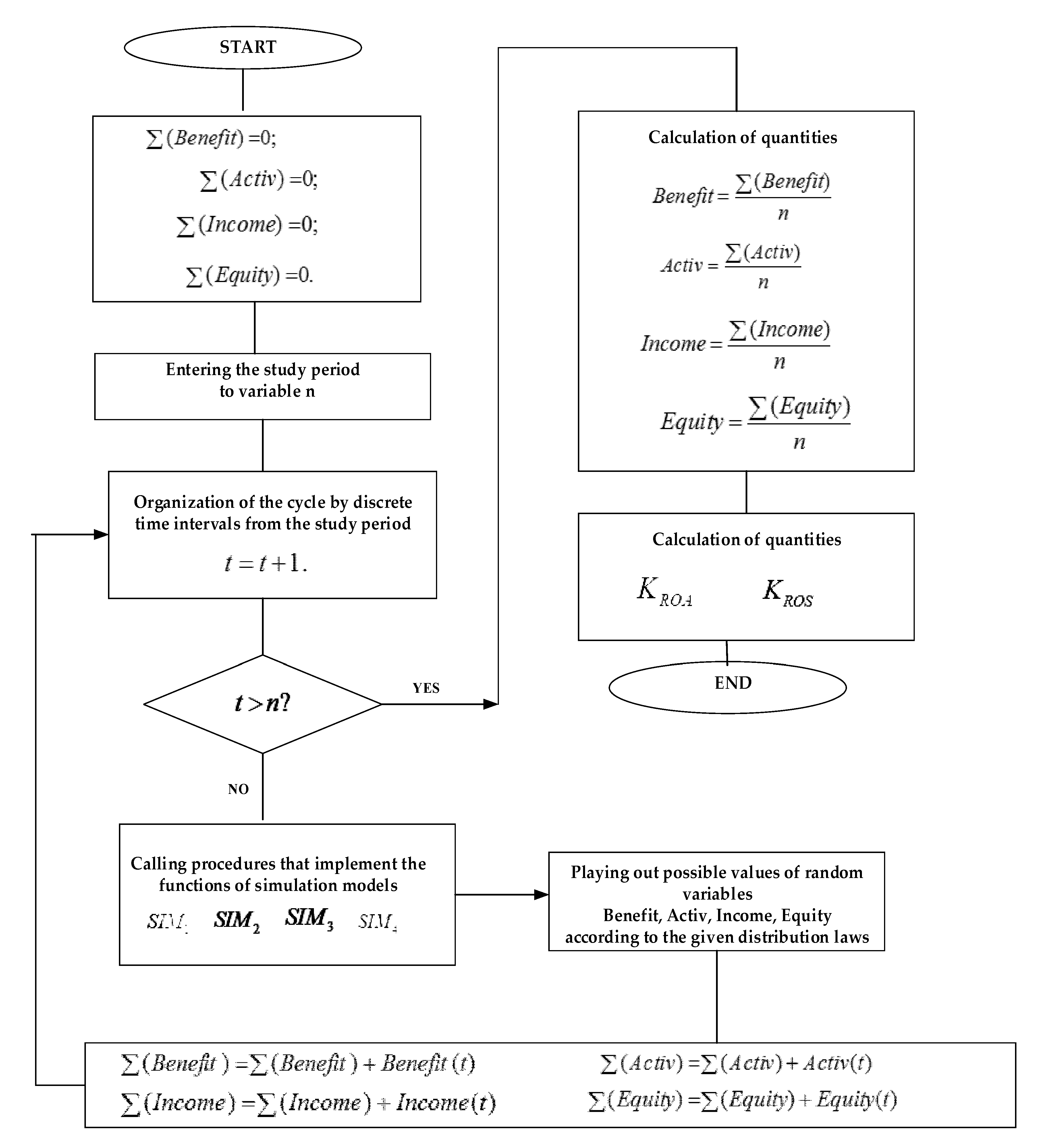
The generated values of the values B e n e f i t , A c t i v , I n c o m e , E q u i t y are used by factor financial analysis models D P 2 , D P 3 , in accordance with the algorithm shown in Figure 2.
The algorithm works as follows. Generation of possible values of random variables B e n e f i t , A c t i v , I n c o m e , E q u i t y at a time according t to the given distribution laws is implemented by simulation models S I M 1 , S I M 2 , S I M 3 , S I M 4 . A loop t is organized by a variable. At the end of the cycle, the generated values are summed in variables ( B e n e f i t ) ; ( A c t i v ) ; ( I n c o m e ) ; ( E q u i t y ) . At the beginning of the cycle, these variables are assigned zero values:
( B e n e f i t ) = 0 , ( A c t i v ) = 0 , ( I n c o m e ) = 0 , ( E q u i t y ) = 0 .
The accumulated amounts are used to calculate the average values
B e n e f i t = ( B e n e f i t ) n , A c t i v = ( A c t i v ) n , I n c o m e = ( I n c o m e ) n , E q u i t y = ( E q u i t y ) n , involved in determining the coefficients K R O A and K R O S .

3.3. Computer Implementation of a Complex of Mathematical Models of Factor Financial Analysis

The proposed set of economic and mathematical models Ω = < i = 1 4 W i , S I M i i = 1 4 , D P 2 , D P 3 > was implemented in the OMEGA software product. The user interface of the OMEGA software package contains menu items: “Input Statistical Data” and “DuPont Model”.
When you click the “Input Statistical Data” button, a drop-down list of “Net Profit”, “Own Capital”,“Revenue”, and “Assets” items appear and activating them invites the researcher to enter statistical data for the corresponding parameters. Pressing the “DuPont Model” button activates the simulation models S I M 1 , S I M 2 , S I M 3 , S I M 4 and models D P 2 , D P 3 The algorithm for the functioning of factor financial analysis models based on the application of the developed software product OMEGA presents the results of financial analysis of the operation of the company PJSC Gazprom. The initial data used in the financial analysis process is shown in Table 2.
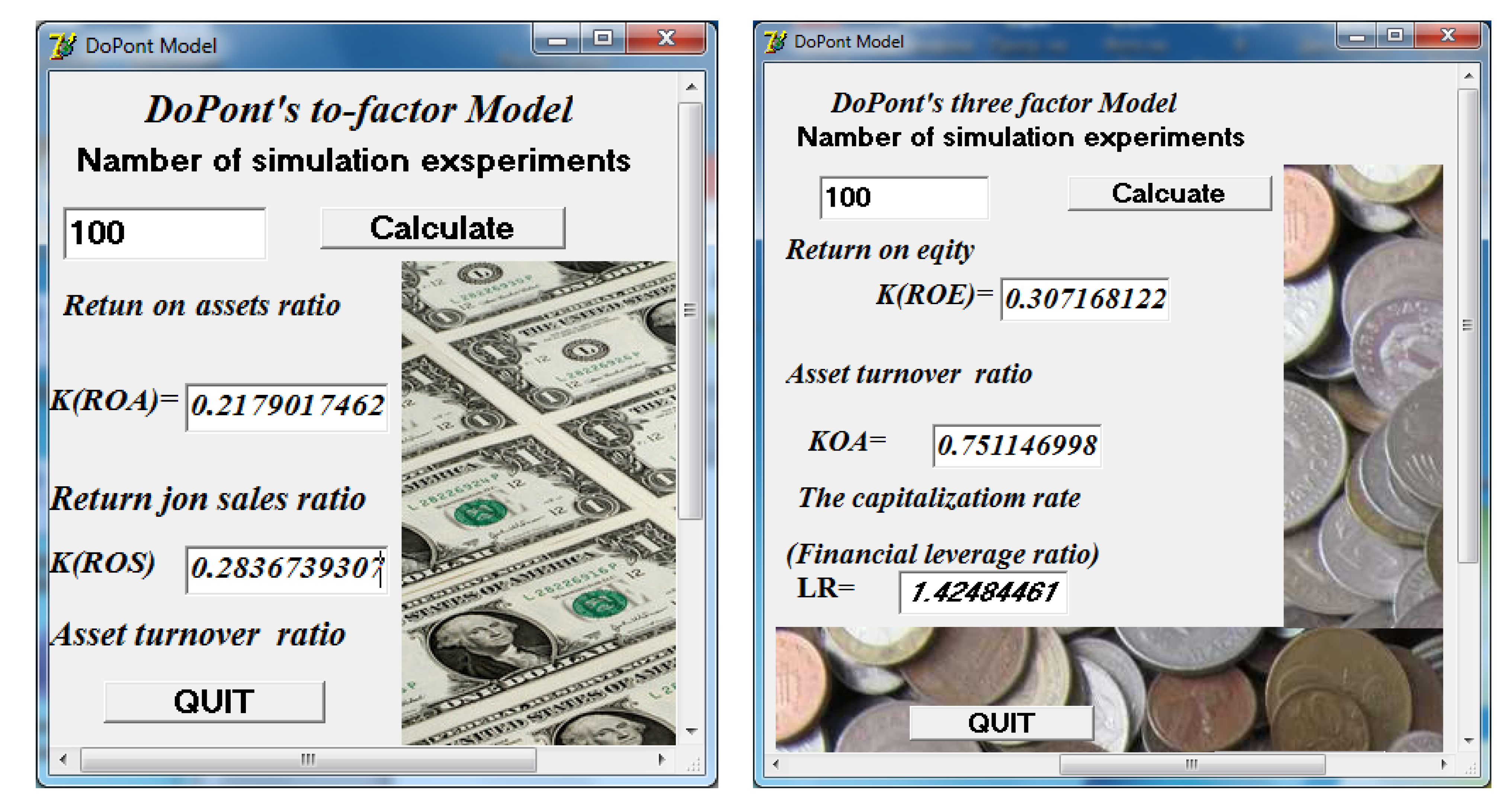
The initial data shown in Table 2 were entered into the OMEGA software product. As a result of statistical processing of the initial data, the laws of distribution of random variables “Net profit”, “Equity”, “Revenue”, and “Assets” were constructed, on the basis of which their forecast values were generated, and the characteristics of two-factor and three-factor analysis were determined. Figure 3 shows the result of the OMEGA program.
Table 3 shows the results of real and model-generated source data.
The generated data were evaluated according to the Fischer criterion. In this case, the generated possible values of random variables B e n e f i t ( t ) , A c t i v ( t ) , I n c o m e ( t ) , E q u i t y ( t ) were compared with the data obtained during a full-scale experiment (Table 3). The null hypothesis that there is no difference between the experimental and generated data was tested by comparing the variances of the experimental data B e n e f i t i , A c t i v i , I n c o m e i , E q u i t y i ,
D ( B e n e f i t ) = i = 1 n ( B e n e f i t i M ( B e n e f i t ) ) 2 n 1 ;   M ( B e n e f i t ) = i = 1 n B e n e f i t i n ;
D ( A c t i v ) = i = 1 n ( A c t i v i M ( A c t i v ) ) 2 n 1 ;   M ( A c t i v ) = i = 1 n A c t i v i n ;
D = i = 1 n ( E q u i t y i M ( E q u i t y ) ) 2 n 1 ;   M ( ω ) = i = 1 n E q u i t y i n ;
with the dispersion of adequacy
D ˜ ( B e n e f i t ) = i = 1 n ( B e n e f i t i B e n e f i t ¯ i ) 2 n 1
D ˜ ( A c t i v ) = i = 1 n ( A c t i v i A c t i v ¯ i ) 2 n 1 ;
D ˜ ( I n c o m e ) = i = 1 n ( I n c o m e i I n c o m e ¯ i ) 2 n 1 ;
D ˜ ( E q u i t y ) = i = 1 n ( E q u i t y i E q u i t y ¯ i ) 2 n 1 ;
where B e n e f i t ¯ i , A c t i v ¯ i , I n c o m e ¯ i , E q u i t y ¯ i —the possible values of the corresponding random variables played using the method of statistical tests according to the given laws of the probability distribution. The degree of equality of variances D ( X ) and D ˜ ( X ) , X { B e n e f i t , A c t i v , I n c o m e , E q u i t y } was evaluated by the Fisher statistical criterion, the calculated value F = D ˜ ( X ) D ( X ) which was compared with the table value F T . Table 4 shows the calculated and tabular values of the Fisher criterion for the studied values B e n e f i t , A c t i v , I n c o m e , E q u i t y .
Table 4 shows a high degree of correspondence between the generated and experimental data since the relation is fulfilled for all random variables F < F T .
Figure 3 shows the result of the OMEGA program.
As a result of two-factor and three-factor analysis, the following characteristics were obtained: return on assets ratio K(ROA) = 0.2179; return on sales ratio K(ROS) = 0.307; asset turnover ratio KOA = 0.75; return on equity K(ROE) = 0.307;capitalization ratio (leverage ratio) LR = 1.425.
The advantage of the constructed models is their ability to minimize the following effects of information asymmetry: objectivity, reliability, complexity, accuracy, relevance, and usefulness. The proposed architecture of factor financial analysis tools (Figure 1), based on the interaction of mathematical models with the database, assumes a constant accumulation of current operational information in the course of the company’s operation and its subsequent computer processing. This reduces the elements of subjectivity, the level of inaccuracy, which contributes to the adoption of correct management decisions that increase the efficiency of the organization’s functioning.

4. Discussion: Complexity of Economics, Mathematical Model, and Open Innovation

This research was focused on the development of a model tool for financial analysis of the functioning of an enterprise that belongs to the class of financial innovations that stimulate the development of the digital economy. The development of digital innovations in the analysis of the functioning of enterprises is currently considered as the main resource that leads them to the innovative trajectory of financial stability. At present, the application of innovations in all areas of enterprise activity has become a central focus of accelerating economic development. At the present stage, information technologies used in the management of small and medium-sized companies [50,51,52,53,54], banking systems [55], consulting organizations [56], etc., have become an actual innovative tool. In the evolution of computer information technologies, as a key factor in the innovative transformation of all spheres of activity of enterprises, the most important role is given to the use of mathematical modeling to solve problems of analyzing the results of their functioning. The economic and mathematical tools developed by the authors were based on the DuPont model, which allows analyzing the dynamics of the profitability of an enterprise in the course of two-factor and three-factor financial analysis. In this case, an interdisciplinary approach was used to synthesize the methods of deterministic financial analysis and simulation modeling. The simulation model was built in the class of discrete-event models and used the following retrospective statistical data as input information: the company’s net profit, the average value of assets, the amount of revenue, the amount of equity. As a result of statistical processing of these data, their probability distribution laws were constructed, which were subsequently used to generate possible values of a random variable using the method of statistical tests. In the course of the research, the adequacy of the constructed economic and mathematical models was evaluated according to the Fisher criterion. At the same time, the generated values of random variables were compared with the data obtained as a result of a full-scale experiment. In accordance with the algorithm of the model, the values of random variables played according to the method of statistical tests were received at the input of the mathematical model of the DuPont factor analysis. The article presented a block diagram of the algorithm for the functioning of economic and mathematical models of factor financial analysis with its subsequent description. The constructed mathematical models were implemented in the software product and included in the innovative technological chain of financial analysis of the enterprise. The article proposed the architecture of the enterprise factor analysis tools, according to which retrospective statistical information is accumulated in the database during the operation of the enterprise and subsequently used for factor financial analysis. Based on the use of the constructed economic and mathematical models, experiments were conducted, the results of which are shown in the corresponding tables of the article. The empirical basis of the study was the data on the functioning of Gazprom. The mathematical models proposed by the authors of this article allow, based on the processing of retrospective data accumulated in the database, the analysis of the financial condition of the enterprise by determining the coefficients of return on equity and assets using the convergence of deterministic and stochastic approaches. The results of the conducted research contribute to the development of innovative tools for conducting financial analysis of enterprises. The constructed mathematical models were implemented in computer programs and integrated into the information technology as a basic component of innovative financial management of the enterprise.

5. Conclusions

Recent events have clearly demonstrated the scientific and practical significance of research devoted to accelerating the economic development of any country, which is based on the use of rapidly developing digital platforms. The development of these platforms poses new challenges not only for business processes but also for their analysis systems, including financial ones. Traditional methods of financial analysis no longer correspond to the changing business environment and require the creation of computer technologies based on mathematical models.
The computer technology proposed by the authors, based on mathematical models, will allow the financial analyst to predict the financial condition of the company based on the analysis of historical information accumulated in the database.

Author Contributions

Conceptualization, A.B.; methodology, I.Y.; software, E.S.; formal analysis, A.N.; writing—original draft preparation, A.K.; writing—review and editing, I.M. All authors have read and agreed to the published version of the manuscript.

Funding

This research received no external funding.

Conflicts of Interest

The authors declare no conflict of interest.

References

  1. Ali, H.F.; Charbaji, A. Applying factor analysis to financial ratios of international commercial airlines. Int. J. Commer. Manag. 1994, 4, 25–37. [Google Scholar] [CrossRef]
  2. Chen, Y.S.; Chen, L.-H.; Liaw, S.-Y. Using financial factors to investigate productivity: An empirical study in Taiwan. Ind. Manag. Data Syst. 2001, 101, 378–384. [Google Scholar] [CrossRef]
  3. Tan, P.M.; Koh, H.C.; Low, L.C. Stability of Financial Ratios: A Study of Listed Companies in Singapore. Asian Rev. Account. 1997, 5, 19–39. [Google Scholar] [CrossRef]
  4. Winand, M.; Zintz, T.; Scheerder, J. A financial management tool for sport federations. Sport Bus. Manag. Int. J. 2012, 2, 225–240. [Google Scholar] [CrossRef] [Green Version]
  5. Tamulevičienė, D.; Mackevičius, J. Methodology of complex analysis of tangible fixed assets. Entrep. Sustain. Issues 2019, 7, 1341–1352. [Google Scholar] [CrossRef]
  6. Timofeeva, N.Y. Forecasting the level of profitability of agricultural products of the Lipetsk region. Mod. Econ. Probl. Solut. 2017, 7, 129–135. [Google Scholar]
  7. Deminova, S.V.; Suchkova, N.A. Forecasting the profitability and sustainability of an organization’s activities using computer modeling. Bull. OrelGIET 2014, 4, 142. [Google Scholar]
  8. Alti, A.; Titman, S. A Dynamic Model of Characteristic-Based Return Predictability. SSRN Electron. J. 2017, 74, 6–3187. [Google Scholar] [CrossRef]
  9. Addoum, J.M.; Delikouras, S.; Korniotis, G.M.; Kumar, A. Income Hedging, Dynamic Style Preferences, and Return Predictability. J. Financ. 2019, 74, 2055–2106. [Google Scholar] [CrossRef]
  10. Bouchaud, J.; Krüger, P.; Landier, A.; Thesmar, D. Sticky Expectations and the Profitability Anomaly. J. Financ. 2018, 74, 639–674. [Google Scholar] [CrossRef]
  11. Weisbrod, E. Stockholders’ Unrealized Returns and the Market Reaction to Financial Disclosures. J. Financ. 2018, 74, 899–942. [Google Scholar] [CrossRef]
  12. Chiang, C.; Dai, W.; Fan, J.; Hong, H.; Tu, J. Robust Measures of Earnings Surprises. J. Financ. 2018, 74, 943–983. [Google Scholar] [CrossRef]
  13. Malloy, C.; Moskowitz, T.; Vissing-Jørgensen, A. Long-run stockholder consumption risk and asset returns. J. Financ. 2009, 64, 2427–2479. [Google Scholar] [CrossRef]
  14. Pastor, L.; Stambaugh, R.F. Predictive Systems: Living with Imperfect Predictors. SSRN Electron. J. 2008, 64, 4–1583. [Google Scholar] [CrossRef] [Green Version]
  15. Livdan, D.; Sapriza, H.; Zhang, L. Financially Constrained Stock Returns. SSRN Electron. J. 2006, 64, 4–1827. [Google Scholar] [CrossRef] [Green Version]
  16. Fama, E.; French, K. The corporate cost of capital and the return on corporate investment. J. Financ. 1999, 54, 1939–1967. [Google Scholar] [CrossRef]
  17. Harford, J. Corporate Cash Reserves And Acquisitions. SSRN Electron. J. 1997, 54, 6–1969. [Google Scholar] [CrossRef]
  18. Easterwood, J.C.; Nutt, S.R. Inefficiency in Analysts’ Earnings Forecasts: Systematic Misreaction or Systematic Optimism? J. Financ. 1999, 54, 1777–1797. [Google Scholar] [CrossRef]
  19. Jiang, F.; Ma, Y.; Wang, X. Multiple blockholders and earnings management. J. Corp. Financ. 2020, 64, 101689. [Google Scholar] [CrossRef]
  20. Sanchis, R.; Duran-Heras, A.; Poler, R. Optimising the Preparedness Capacity of Enterprise Resilience Using Mathematical Programming. Mathematics 2020, 8, 1596. [Google Scholar] [CrossRef]
  21. Cerna, S.; Guyeux, C.; Royer, G.; Chevallier, C.; Plumerel, G. Predicting Fire Brigades Operational Breakdowns: A Real Case Study. Mathematics 2020, 8, 1383. [Google Scholar] [CrossRef]
  22. Vasylieva, T.; Jurgilewicz, O.; Poliakh, S.; Tvaronavičienė, M.; Hydzik, P. Problems of measuring country’s financial security. J. Int. Stud. 2020, 13, 329–346. [Google Scholar] [CrossRef]
  23. Hilkevics, S.; Semakina, V. The classification and comparison of business ratios analysis methods. Insights Reg. Dev. 2019, 1, 48–57. [Google Scholar] [CrossRef] [Green Version]
  24. Shahi, T.B.; Shrestha, A.; Neupane, A.; Guo, W. Stock Price Forecasting with Deep Learning: A Comparative Study. Mathematics 2020, 8, 1441. [Google Scholar] [CrossRef]
  25. Espinoza-Audelo, L.F.; Olazabal-Lugo, M.; Blanco-Mesa, F.; León-Castro, E.; Alfaro-Garcia, V. Bonferroni Probabilistic Ordered Weighted Averaging Operators Applied to Agricultural Commodities’ Price Analysis. Mathematics 2020, 8, 1350. [Google Scholar] [CrossRef]
  26. Borodin, A.; Mityushina, I. Evaluating the effectiveness of companies using the DEA method. Nauk. Visnyk Natsionalnoho Hirnychoho Universytetu 2020, 6, 193–197. [Google Scholar] [CrossRef]
  27. Streltsova, E.; Yakovenko, I. Support of Dicision-Making in Interbudgetary Regulation on the Basis of Simulation Modeling. Smart Innov. Syst. Technol. 2019, 139, 165–172. [Google Scholar]
  28. Selvachandran, G.; Ngan, T.T.; Sharma, R. Similarity Measure of Lattice Ordered Multi-Fuzzy Soft Sets Based on Set Theoretic Approach and Its Application in Decision Making. Mathematics 2020, 8, 1255. [Google Scholar] [CrossRef]
  29. Lamothe-Fernández, P.; Alaminos, D.; Lamothe-López, P.; Fernández-Gámez, M.A. Deep Learning Methods for Modeling Bitcoin Price. Mathematics 2020, 8, 1245. [Google Scholar] [CrossRef]
  30. Szetela, B.; Mentel, G.; Mentel, U.; Bilan, Y. Directional Movement Distribution in the Bitcoin Markets. Eng. Econ. 2020, 31, 188–196. [Google Scholar] [CrossRef]
  31. Meng, Y.; Qasem, S.N.; Shokri, M.S. Dimension Reduction of Machine Learning-Based Forecasting Models Employing Principal Component Analysis. Mathematics 2020, 8, 1233. [Google Scholar] [CrossRef]
  32. Popkov, Y.S.; Popkov, A.Y.; Dubnov, Y.A.; Solomatine, D. Entropy-Randomized Forecasting of Stochastic Dynamic Regression Models. Mathematics 2020, 8, 1119. [Google Scholar] [CrossRef]
  33. Chiu, M.-C.; Chen, T.-C.T.; Hsu, K.-W. Modeling an Uncertain Productivity Learning Process Using an Interval Fuzzy Methodology. Mathematics 2020, 8, 998. [Google Scholar] [CrossRef]
  34. Jiang, P.; Hu, Y.-C.; Wang, W.; Jiang, H.; Wu, G. Interval Grey Prediction Models with Forecast Combination for Energy Demand Forecasting. Mathematics 2020, 8, 960. [Google Scholar] [CrossRef]
  35. Suganthi, L.; Samuel, A.A. Energy models for demand forecasting—A review. Renew. Sustain. Energy Rev. 2012, 16, 1223–1240. [Google Scholar] [CrossRef]
  36. Ediger, V.Ş.; Akar, S. ARIMA forecasting of primary energy demand by fuel in Turkey. Energy Policy 2007, 35, 1701–1708. [Google Scholar] [CrossRef]
  37. González, P.A.; Zamarreño, J.M. Prediction of hourly energy consumption in buildings based on a feedback artificial neural network. Energy Build. 2005, 37, 595–601. [Google Scholar] [CrossRef]
  38. Tutun, S.; Chou, C.-A.; Canıyılmaz, E. A new forecasting framework for volatile behavior in net electricity consumption: A case study in Turkey. Energy 2015, 93, 2406–2422. [Google Scholar] [CrossRef]
  39. Lauret, P.; Fock, E.; Randrianarivony, R.N.; Manicom-Ramsamy, J.-F. Bayesian neural network approach to short time load forecasting. Energy Convers. Manag. 2008, 49, 1156–1166. [Google Scholar] [CrossRef]
  40. Wang, C.-H.; Hsu, L.-C. Using genetic algorithms grey theory to forecast high technology industrial output. Appl. Math. Comput. 2008, 195, 256–263. [Google Scholar] [CrossRef]
  41. Cui, J.; Liu, S.-F.; Zeng, B.; Xie, N.-M. A novel grey forecasting model and its optimization. Appl. Math. Model. 2013, 37, 4399–4406. [Google Scholar] [CrossRef]
  42. Hu, Y.-C.; Tseng, F.-M. Functional-link net with fuzzy integral for bankruptcy prediction. Neurocomputing 2007, 70, 2959–2968. [Google Scholar] [CrossRef]
  43. Nieto, P.J.G.; Gonzalo, E.G.; Lasheras, F.S.; Sánchez, A.B. A Hybrid Predictive Approach for Chromium Layer Thickness in the Hard Chromium Plating Process Based on the Differential Evolution/Gradient Boosted Regression Tree Methodology. Mathematics 2020, 8, 959. [Google Scholar] [CrossRef]
  44. Zhou, Y.; Zhou, M.; Xia, Q.; Hong, W.-C. Zhou Construction of EMD-SVR-QGA Model for Electricity Consumption: Case of University Dormitory. Mathematics 2019, 7, 1188. [Google Scholar] [CrossRef] [Green Version]
  45. Shih, P.-C.; Chiu, C.-Y.; Chou, C.-H. Using Dynamic Adjusting NGHS-ANN for Predicting the Recidivism Rate of Commuted Prisoners. Mathematics 2019, 7, 1187. [Google Scholar] [CrossRef] [Green Version]
  46. Blackledge, J.; Kearney, D.; Lamphiere, M.; Rani, R.; Walsh, P. Econophysics and Fractional Calculus: Einstein’s Evolution Equation, the Fractal Market Hypothesis, Trend Analysis and Future Price Prediction. Mathematics 2019, 7, 1057. [Google Scholar] [CrossRef] [Green Version]
  47. Ermakov, S.; Leora, S. Monte Carlo Methods and the Koksma-Hlawka Inequality. Mathematics 2019, 7, 725. [Google Scholar] [CrossRef] [Green Version]
  48. Afanasyev, D.O.; Fedorova, E.A. On the impact of outlier filtering on the electricity price forecasting accuracy. Appl. Energy 2019, 236, 196–210. [Google Scholar] [CrossRef]
  49. Zelenkov, Y.; Fedorova, E.; Chekrizov, D. Two-step classification method based on genetic algorithm for bankruptcy forecasting. Expert Syst. Appl. 2017, 88, 393–401. [Google Scholar] [CrossRef]
  50. Prendes-Espinosa, P.; Solano-Fernández, I.; García-Tudela, P. EmDigital to Promote Digital Entrepreneurship: The Relation with Open Innovation. J. Open Innov. Technol. Mark. Complex. 2021, 7, 63. [Google Scholar] [CrossRef]
  51. Oudgou, M. Financial and Non-Financial Obstacles to Innovation: Empirical Evidence at the Firm Level in the MENA Region. J. Open Innov. Technol. Mark. Complex. 2021, 7, 28. [Google Scholar] [CrossRef]
  52. Jeong, H.; Shin, K.; Kim, E.; Kim, S. Does Open Innovation Enhance a Large Firm’s Financial Sustainability? A Case of the Korean Food Industry. J. Open Innov. Technol. Mark. Complex. 2020, 6, 101. [Google Scholar] [CrossRef]
  53. Jin, S.; Lee, K. The Government R&D Funding and Management Performance: The Mediating Effect of Technology Innovation. J. Open Innov. Technol. Mark. Complex. 2020, 6, 94. [Google Scholar] [CrossRef]
  54. Leitão, J.; Pereira, D.; De Brito, S. Inbound and Outbound Practices of Open Innovation and Eco-Innovation: Contrasting Bioeconomy and Non-Bioeconomy Firms. J. Open Innov. Technol. Mark. Complex. 2020, 6, 145. [Google Scholar] [CrossRef]
  55. Rashid, H.U.; Nurunnabi, M.; Rahman, M.; Masud, A.K. Exploring the Relationship between Customer Loyalty and Financial Performance of Banks: Customer Open Innovation Perspective. J. Open Innov. Technol. Mark. Complex. 2020, 6, 108. [Google Scholar] [CrossRef]
  56. Méndez-Suárez, M.; García-Fernández, F.; Gallardo, F. Artificial Intelligence Modelling Framework for Financial Automated Advising in the Copper Market. J. Open Innov. Technol. Mark. Complex. 2019, 5, 81. [Google Scholar] [CrossRef] [Green Version]
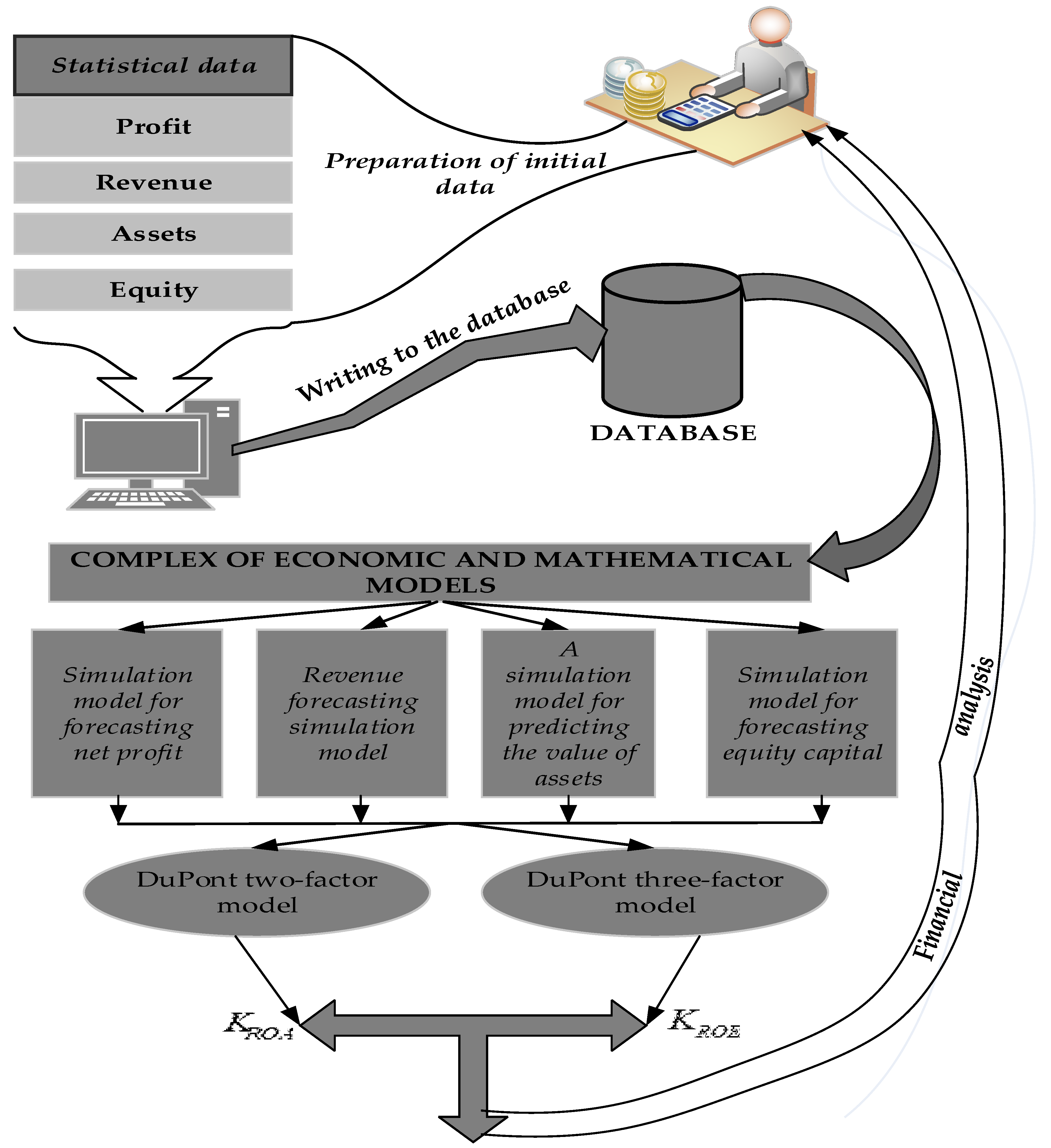
Figure 1. The architecture of the Toolkit the factorial financial analysis.
Joitmc 07 00079 g001
Figure 2. The algorithm of functioning of factor models for financial analysis D P 2 , D P 3 .
Joitmc 07 00079 g002
Figure 3. The results of factor analysis of financial.
Joitmc 07 00079 g003
Table 1. Laws of distribution of random variables B e n e f i t , A c t i v , I n c o m e , E q u i t y .
R(Benefit)IntervalsBen1Ben2Benm
Relative frequencyP(Benefit1)P(Benefit2)P(Benefitm)
R(Activ)IntervalsAc1Ac2Acm
Relative frequencyP(Activ1)P(Activ2)P(Activm)
R(Income)IntervalsIn1In2Inm
Relative frequencyP(Income1)P(Income2)P(Incomem)
R(Equity)IntervalsEq1Eq2Eqm
Relative frequencyP(Equity1)P(Equity2)P(Equitym)
Table 2. Statistical data for factor analysis of the functioning of the PJSC Gazprom.
YearNet ProfitEquity CapitalRevenueAssets
2007360,449,5504,663,465,9901,774,959,4375,929,361,713
2008173,021,6304,773,520,5982,507,009,5046,181,534,689
2009624,613,2735,398,689,4192,486,940,6186,950,737,357
2010364,478,3826,187,890,2342,879,390,3247,828,107,263
2011879,601,6647,539,089,8953,534,341,4319,521,274,120
2012556,387,1697,883,295,4783,659,150,75710,035,900,474
2013628,311,2218,369,165,4603,933,335,31310,855,186,062
2014188,980,0169,089,213,1203,990,280,17212,249,735,124
2015403,522,8069,322,338,8404,334,293,47712,981,247,957
2016411,424,59710,414,000,2473,934,488,44113,852,945,759
2017100,297,97710,324,208,3704,313,031,61614,385,169,353
Table 3. Conformity assessment experienced and generated by the method of statistical tests the original data.
Net ProfitEquity CapitalRevenueAssets
Real DataThe Generated DataReal DataThe Generated DataReal DataThe Generated DataReal DataThe Generated Data
360,449,550320,542,6704,663,465,9903,992,167,3811,774,959,437893,211,6215,929,361,7133,884,564,529
173,021,630184,011,4504,773,520,5985,124,125,8702,507,009,504998,115,4126,181,534,6895,223,876,561
624,613,273529,824,2825,398,689,4194,284,363,8822,486,940,6181,754,671,5236,950,737,3574,881,563,761
364,478,382392,253,6716,187,890,2347,003,001,4202,879,390,3242,111,431,9127,828,107,2637,337,817,825
879,601,66477,510,4327,539,089,8957,176,401,5673,534,341,4312,992,317,8499,521,274,1208,991,113,610
556,387,169235,272,0987,883,295,4786,376,832,6533,659,150,7572,932,581,43810,035,900,4746,345,145,356
628,311,221439,221,3838,369,165,4606,654,216,5713,933,335,3132,299,928,72710,855,186,06211,167,567,481
188,980,016211,471,0579,089,213,1208,872,925,4113,990,280,1723,000,181,35712,249,735,12419,949,783,765
403,522,806296,319,7149,322,338,8406,221,546,7214,334,293,4773,873,169,84712,981,247,95713,825,001,345
411,424,597383,517,32910,414,000,2479,837,110,1643,934,488,4413,111,258,32513,852,945,75919,457,656,731
100,297,977111,224,31510,324,208,3708,656,435,6514,313,031,6164,313,031,61614,385,169,35321,376,574,674
Table 4. Values of the Fisher criterion for estimating statistical proximity of variances D ( X ) and D ˜ ( X ) , X { B e n e f i t , A c t i v , I n c o m e , E q u i t y } .
Benefit Activ Income Equity
F F T F F T F F T F F T
1.49871.841.741.841.42351.840.4611.84
Publisher’s Note: MDPI stays neutral with regard to jurisdictional claims in published maps and institutional affiliations.