Abstract
The peak power of the manufacturing systems can increase electricity costs and reduce the use of renewable energy suppliers. The power of the machining processes depends on the processing time of the operations. Then, the allocation of the power to the machines of a manufacturing system controls the processing time of the manufacturing operations. An efficient allocation model can reduce the peak power, keeping the throughput performance level. This paper proposes a game theory to allocate the power to the machines including the dependence of the processing time from the power allocated. The game model uses the Gale-Shapley algorithm that forms couples of under and overloaded machines. Then, each couple exchanges the power from the underloaded to overloaded machines. The model considers the global workload and the jobs in queue for each machine. A simulation model tests the proposed method compared to a benchmark where each machine works with fixed power. The simulation results show how the model can improve the performance of the manufacturing system in several conditions tested. In particular, the main benefits can be obtained when the manufacturing system has high or medium utilization or the uncertainty affects the processing time.
1. Introduction
The new legislation, national reduction targets and cost pressure drive the production companies to improve the energy efficiency [1].
Recent international research denoted an increment of the world industrial energy consumption by 3.4% annually until 2040 [2]. Manufacturing activities consume a third of the total energy produced in the United States and a quarter in Europe [3,4].
The investment to satisfy the demand during peak periods can be more relevant; Faruqui et al. [5] estimated that the cost in the United States due to the peak demand of only 100 hours of the year is between 10% and 20% of electricity cost.
The traditional approaches to design and control of manufacturing systems do not take into account the energy reduction target. In recent years, the introduction of energy reduction focus worsens the other indicators, such as throughput, work in process, etc.
One field of the research concerns the reduction in energy consumption in manufacturing systems considering the switch-off of the machines [6,7,8]. The introduction of buffers is necessary to keep the throughput target of the system.
Another problem is the peak power consumption because the power consumption at any time should not exceed a maximum quantity. The load balancing and the minimization of the peak power can contribute significantly to reducing the energy costs (energy supplier or penalty costs). In the case of a manufacturing system composed of CNC machines, the power consumption impacts on the processing time. In particular, when the processing time decreases, the power consumption increases.
Moreover, the smoothing of the machines’ power load can improve the use of renewable energy as a photovoltaic array [9].
The off-line and on-line approaches can support the control and reduction in the peak power in manufacturing systems. The off-line approaches concern the use of predictive scheduling that includes energy issues. These approaches cannot face unforeseen events such as production demand, renewable energy outputs, etc. [10]. The on-line approaches assure the performance of the manufacturing system when the system condition dynamically changes [11].
Some works proposed a real-time control of the machines to determine the start of the operations to control the peak load [9]. Other works proposed scheduling approaches based on heuristic algorithms, such as a genetic algorithm, simulated annealing, artificial neural networks, etc. [12,13,14].
These approaches considered the energy improvements, but restricted manufacturing system performance measures are evaluated. The computational complexity of these models limits the potential application of real-time control in manufacturing systems when the number of machines increases. Moreover, the fourth industrial revolution drives the use of cloud computing, Big data, Internet of Things and the reduced computational complexity and open innovation are key success factors in this context [15].
Open innovation is defined as follows: “open innovation is a paradigm that assumes that firms can and should use external ideas as well as internal ideas, and internal and external paths to market, as the firms look to advance their technology [16]”. These infrastructures are necessary to manage complex manufacturing systems and develop algorithms for improving flexibility and saving costs.
This paper proposes the real-time control of the energy consumption of flexible manufacturing systems. The model works in quasi real-time to allocate the power available to the machines evaluating the system conditions. The power allocated to the machine determines the processing time of the machine and the performance.
The power allocation among the machines has a peak constraint of the manufacturing system. The approach developed is similar to a cooperation mechanism among the machines to share the total power of the system as a limited resource. The cooperation mechanism proposed is based on a game theory model. The game model ensures a limited computational complexity that allows supporting the more complex manufacturing system. A simulation model is used to test the proposed model and evaluates several performance measures with fixed peak power.
The paper is structured as follows. The past works proposed in the literature on power allocation in manufacturing systems are discussed in Section 2. Section 3 introduces the Gale–Shapley algorithm and manufacturing system architecture. The experimental simulation characteristics are described in Section 4. The discussion of the numerical results is provided in Section 5, while Section 6 explains the main conclusions and highlights some future research directions.
2. Literature Review
The scheduling problem in job shop systems focused on improving the production performance, reducing production costs [17]. Over the last few years, the reduction in costs has included the reduction in energy consumption in manufacturing systems [18].
Scheduling models may include energy consumption, but beyond a few machines, the problem is difficult to solve. The applications of the mathematical models proposed in the literature are suitable for small cases, while the heuristic approaches can be applied in real industrial cases [18,19]. These models allocate tasks to reduce energy consumption.
Another research field in reducing energy consumption is the switch off policy to reduce the standby energy of the machines, introducing buffers. These models control the switch-off of the machines when the upstream buffer is empty or the downstream buffer reaches a maximum level. These approaches need an adequate buffers’ level to reduce the impact on throughput [6,7].
Few works have been concerned with the real-time load management of the machines to reduce peak load to respect the constraints of the maximum power energy available, including those depending on the processing time by the power. Módos et al. [20] studied the scheduling on a single machine with an energy consumption limit. They proposed logic-based Benders decomposition, Branch-and-Bound algorithms and one heuristic algorithm (Tabu-Search). These algorithms are complex, used on a single machine and small instances; therefore, these models are not applicable in real industrial cases.
Several works focused on flowlines to reduce the peak power with the introduction of a buffer and switch-off policy of the machines. Sun and Li [21] proposed a Markovian model in flow shop systems to reduce the power load of the manufacturing system without impact on the throughput. They introduced buffers in a flow line to reduce the energy consumption of some machines by the switch off or reducing the energy of the process.
Fernandez et al. [22] proposed the introduction of the buffer in a flow line to reduce the energy consumption during peak periods under the constraint of system throughput. When the downstream buffer reaches a defined level, the machine can be switched off. A similar approach was proposed in Sun et al. [23], who studied the introduction of the buffer to reduce electricity consumption during peak periods in flowline systems. In this case, the costs of the buffer and the failure of the machines were considered. Nagasawa et al. [24] proposed a model to reduce the peak power consumption in flow shop systems under uncertain processing times of the operations. The scheduling approach proposed inserts idle times to reduce the peak power of the system. The computational time of the algorithm proposed can increase significantly with the size of the system. Wang and Wang [25] studied a flow shop to solve the scheduling problem with peak power consumption constraints and minimize the makespan. They proposed five decoding methods to yield good schedules from a job permutation.
Other works considered the introduction of renewable energy as an energy source for the manufacturing system. Beier et al. [26] proposed a real-time energy flexibility control to align manufacturing system energy control variable renewable energy supply without compromising throughput. The manufacturing system considered was a flow line with the introduction of the buffer and a control strategy to switch off the machines.
Few works proposed models in a job-shop context; Liu et Al. [18] proposed a scheduling model in job-shop manufacturing to minimize the total electricity consumption and total weighted tardiness. The model proposed was tested in a very simplified context with 10 jobs and 10 machines; this limits the application in real industrial applications.
Popp and Zhae [27] proposed a framework to investigate the influence of the machines on the energy demand. The objective is to determine the machines where the energy can reduce the product quality to determine the manufacturing system part to control without a negative effect on the performance.
Schultz et al. [28] studied a short-term production control where the electric energy is considered as limited production capacity. The objective is to align energy demand in production with energy supply while maintaining logistic goals.
Some works focused on the electric load forecast. The models proposed are based on several heuristic methods, such as the Hybrid Self-Recurrent Support Vector Regression Model with variational mode decomposition and Improved Cuckoo Search Algorithm, and the hybrid chaotic immune algorithm. These models are applied in civil context and for the production of electric energy. A potential field of application of these models can be the introduction of renewable energy supplies in manufacturing systems [29,30,31,32,33].
Gajic et al. [13] proposed a MILP production planning model to reduce electricity consumption in a real melt shop. The reduction in terms of costs obtained is around 3%.
The major part of the research focused on a single machine or flow shop. However, in real industrial cases, job shop systems have significant relevance. The models proposed in the literature are characterized by relevant computational complexity that reduces the applicability to a few machines. This limits the possibility to extend these methods to real industrial cases. Nowadays, the manufacturing companies need to cooperate to improve efficiency; the proposed method is suitable to promote the cooperation among enterprises to allocate power and reduce the energy costs. In this context, the use of the open innovation models helps the enterprises to use the emerging technologies to improve energy and resource efficiency of industrial production [34,35].
Lee et al. [36] and Hossain and Kauranen [37] discussed an overview of the open innovation models used in small and medium enterprises (SMEs) to overcome traditional cooperation approaches and generate value added for the partners. These models based on the development of intelligent automation systems, such as smart factories, gain benefit from the application of open innovation [38,39,40]. Moreover, game theory is a promised method to support open innovation model as shown in the work of Yun et al. [41]. The resource integration can gain relevant benefit from the adoption of open innovation models [42].
This paper proposes a model that limits the computational workload allowing the applicability in real industrial cases with complex manufacturing systems. This approach works as a cooperation method among the machines that share the power available as a limited resource. The cooperation model collects the state of each machine and allocates the power among the machine under a peak constraint. Therefore, the model proposed to pursue the improvement of the performance, reducing the peak power needed.
A game theory model based on the Gale–Shapley algorithm supports cooperation among the machines. The capacity cooperation [43] and the reconfigurable manufacturing systems [44] were some examples of cooperation models based on the Gale–Shapley algorithm.
Any works based on game theory were proposed to support manufacturing systems under peak power load. Then, the first research question of this paper is the following:
RQ1: What is the impact of the cooperation model based on the Gale–Shapley algorithm on the performance of a job shop manufacturing system?
The second research question regards the possibility to reduce the peak power keeping the same performance of the manufacturing system:
RQ2: Can the peak power load reduce without negative effect on the performance of the manufacturing system?
3. Reference Context
The model considered is a job shop system where the jobs have a random routing sequence with a due date assigned. The main assumptions of the manufacturing system are the following:
- Operations cannot be pre-empted;
- Each machine can process only one task at once;
- The queues are managed by the earliest due date (EDD) policy to improve the lateness performance.
In this research, the material handling time is included in the machining time, and the handling resources are always available. This reference context was used in previous works for workload control research [45].
The notation is the following:
M = 1, M is the index of the machines or work centers (the terms can be interchangeable);
i is the index of the generic part enters in the manufacturing system
aim = 1 if the part i requires the operation of the machine m, 0 otherwise;
Topim is the process time of the part i in the machine m
WLm is the workload of the machine/work center m;
WLqm is the sum of the processing time of the part in queue in the machine/work center m;
WLeqm is an equivalent workload computed for each machine/work center m;
WLav is the average of the workload equivalent over all machines/work centers;
U is the cardinality of the under-loaded set of machines;
O is the cardinality of the over-loaded set of machines;
U = 1, U is the index of the under-loaded machines’ set;
O = 1, O is the index of the over-loaded machines’ set;
RWLo is the difference of the workload of the machine o in the over-loaded set to the WLav;
OWLu is the difference of the workload of the machine u in the under-loaded set to the WLav;
Uo,u is the preference (Gale-Shapley model) of the member o of the over-loaded set for the u member of the under-loaded set;
Uu,o is the preference (Gale-Shapley model) of the member u of the under-loaded set for the o member of the over-loaded set;
Tp is the period time fixed to evaluate the reconfiguration of the machines.
α is the weight of the workload WLm to compute the workload equivalent;
β is the weight of the workload WLqm to compute the workload equivalent;
Powm is the power allocated to the machine/work center m;
Pmaxm is the maximum power for the machine/work center m;
Pminm is the minimum power for the machine/work center m;
3.1. Energy Consumption Model
The allocation of the power to the machines determines the cutting speed and, therefore, the processing time of the task for the jobs. An energy consumption model is necessary to define the relationship between power and the cutting speed. The energy consumption model used in this research is the same as that proposed in Kara and Li [46] and Anderberg et al. [47]. In brief, the main equations used in this research are explained. Equation (1) computes the specific energy consumption (SEC) of the machine:
where C0 and C1 are the specific machine coefficients and MRR [cm3/sec] is the material remove rate. The SEC is a functional unit that is the energy consumed to remove 1 cm3 of material; this is allowed to compare the energy consumption under different cutting conditions. Empirical experiments conducted on the manufacturing machines determine the parameters C0 and C1. The material removal rate (MRR) is the amount of material removed from the workpiece per unit time.
The power of the machine is determined by Equation (2):
where P0 [kw] is the fixed power consumption when the machine is in a standby state.
Equation (3) describes the processing time (PT) of the operation.
where,
where,
p is the deep of cut;
D is the diameter of the tool;
L is the length of the cutting operation.
The above model allows obtaining the processing time of the machine for the power allocated. Then, the generic CNC machine controls the processing time based on the power available.
3.2. Approach Proposed
The cooperation mechanism proposed shares power among the machines. Then, the model forms a couple of machines to share power. The Gale–Shapley algorithm supports this model [48]. The original model denotes two sets of agents, called men and women, with the same size. Every agent has a complete list of preferences for the opposite sex. The Gale–Shapley algorithm finds stable couples among men and women. A complete description of the algorithm and applications can be found in Renna [44], Gale and Shapley [48], Kobayashi and Matsui [49]. The Gale–Shapley algorithm is characterized by low computational complexity and this algorithm demonstrated the aptitude for short-term decisions [50].
The Gale–Shapley algorithm needs to be adapted to support the power allocation among the machines of the manufacturing system. The processing time of the technological operations depends on the power allocated to the machine. The Gale–Shapley algorithm works on two sets defined men and women; therefore, the machines that compose the manufacturing system should be divided into men and women for analogy.
The following decision is necessary to use the Gale–Shapley Algorithm:
- -
- What are the conditions that make a machine belong to the men or women set;
- -
- How preferences are calculated among the components of the two sets.
A machine belongs to men or women set considering the workload within the manufacturing system (global information) and the parts in the queue of the machines (local information). Each part that enters in the manufacturing systems obtains the (aim) and process time (Topim) following the parameters described in Section 4.
Then, the workload of each machine m (WLm) increases by adding the workload due to the new part in the manufacturing system as shown in Equation (6):
When the part i leaves the machine m and the workload of the machine m is decreased by the Topim, then, the total processing time of the parts in the queue (Q) of the machine m is evaluated, as shown in Equation (7):
Then a weighted average between the two workloads is computed (Equations (6) and (7)):
where .
The WLeqm takes into account the local information of the machine m (the queue) and the global information, that is, the workload of the machine m, due to the parts in other machines that will visit the machine m.
The machines are divided into two sets: over-loaded machines OL (men) and under-loaded machines UL (women).
The average equivalent workload (Equation (8)) of the work centers is computed when the power allocation is evaluated (after a Tp period, Equation (9)).
If the workload of the m-machine is lower than WLav, then m ∊ UL set;
If the workload of the m-machine is higher than WLav, then m ∊ OL set;
For each member of the sets OL and UL, the following equations are computed:
Equation (10) computes the power requested (RWLo) by the member o of the over-loaded machine. The request is calculated multiplying a percentage value by difference between the maximum power (Pmaxm) and the power of the machine m (Powm). The percentage value is the percentage difference between the WLeqm of machine m and the average workload WLav.
Equation (9) computes the power that under-loaded machine can offer (OWLu).
The offer is calculated multiplying a percentage value by the difference between the power of the machine m (Powm) and the minimum power (Pminm). The percentage value is the percentage difference between the average workload WLav and the WLeqm of machine m.
The preferences of the men and women are computed using the utility functions as shown in Equations (12) and (13).
The ghost member is necessary when the men and women are not equal, while the Gale–Shapley algorithm works with a symmetric condition (value −1 in Equations (12) and (13)). If the model forms a couple with a ghost member, this couple is not considered as a valid solution.
Then, Equations (12) and (13) mean that the preference is higher when the difference between the power offered and requested is lower. The algorithm of Gale–Shapley iterates until one man or one woman is still free. At the end of the algorithm, a couple of machines to exchange power from the under-loaded to the over-loaded is made.
The power allocation model follows a periodic review policy; every Tp period, the algorithm starts to re-allocate the power among the machines.
The algorithm works through the following steps every Tp time (periodic policy, see Figure 1):
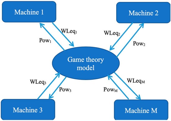
Figure 1.
Game Theory Model.
- Each machine communicates to the centralized decision support model the equivalent workload computed, as shown in Equation (8).
- Then, the decision support model applies the Gale–Shapley model to decide the power for each machine;
- At the end of the computation of the Gale–Shapley model, the power allocated is communicated to each machine.
- The power allocated determines the processing time of the machines.
The real industrial application can be supported by a multi-agent architecture that is more relevant in the actual industry 4.0 [51].
4. Simulation Model
The job shop consists of six work centers, and each work center is characterized by one machine.
When a part is assigned the operations following a discrete uniform distribution (between 1 and 6), the routing follows a random sequence of the operations assigned. The inter-arrival time of the part follows an exponential distribution.
The information about the machine consumption model is reported in [30]; the first simulation to test the proposed approach considers the same technological operation for all the machines with the following data:
- -
- Fadal VMC 4020 [30]: C0 = 2.845, C1 = 1.330 and P0 = 0.74.
- -
- D = 30 mm, p = 5 mm, a = 1.2 mm/revolution, L = 2000 mm.
The appendix reports the table with the correspondence between the power and the processing time.
The following performance measures permit the evaluation of the manufacturing system.
- -
- Three performance measures are used to evaluate the ability to deliver the job on time: percentage of tardy jobs; the standard deviation of lateness; average lateness [unit time]. The standard deviation allows evaluating the fluctuation of the delivery time related to the due date.
- -
- Throughput [parts/unit time]: the total number of items produced by the manufacturing system.
- -
- Average system time [unit time]: the average time from the enter time of the job in the manufacturing system and the exit from its.
- -
- Work in process (WIP) [parts]: the average total parts in the system (the sum of the queues and parts in the machines);
- -
- Average machines’ utilization [a-dimensional]: the average utilization of the machines that compose the manufacturing system;
- -
- Bottleneck shiftness: this index describes the propensity of a bottleneck to shift among work centers as defined in [52].
The statistical analysis of the simulation is conducted following the terminating analysis approach. The simulation length is 25,000 time units. For each experiment class, a number of replications able to assure a 5% confidence interval and 95% of a confidence level for each performance measure conducted. To assure these parameters each experiment class conducted needed over 3000 replications with about 12 hours of computation time (4 GHz Intel Core i7 and 16 Gb RAM).
Different power levels of the manufacturing system (see Table 1) characterize the simulation experiments. Three different values are considered 30, 36 and 42 KW; the manufacturing system consists of six machines, then, the mean power for each machine is, respectively, 5, 6 and 7 Kw.

Table 1.
Simulation parameters.
To keep the same average utilisation, the inter-arrival time is adapted when the power available changes for the manufacturing system.
All the simulations described above are repeated in the case of process uncertainty and the introduction of a bottleneck in the manufacturing system. Moreover, the simulations are repeated for different values of Tp. The value of Tp that leads to better results is always Tp = 5.
Finally, the single machine can operate with a maximum power of 9 Kw and a minimum of 4 KW (see Appendix A).
5. Numerical Results
The numerical results are reported as the percentage difference with the benchmark. The benchmark assigns a fixed power to each machine distributed equally for each case considered (30, 36 and 42 KW). Figure 2 shows the main performance measures evaluated.
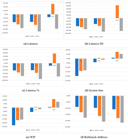
Figure 2.
Simulation results. (a): Lateness; (b): Standard Deviation of the Lateness; (c): percentage of parts in lateness; (d): throughput time of the manufacturing system; (e): Work In Process; (f): Bottleneck shiftness.
The delivery job in time indicators (lateness, lateness DS and lateness %) have the same behavior. There are significant improvements in these measures, in particular, in the cases of int1 and int2. When the inter-arrival time is higher (int3) the benefits are important with higher power available. These performance measures get worst with the combination of higher inter-arrival and medium power available.
The throughput times of the system and the WIP are very similar. The benefits are relevant with lower inter-arrival time (int1) and greater when the power available is lower. The reduction in the bottleneck shift is important in every case tested and it is greater with higher power available.
These results suggest how the proposed method enables improving the performance of the manufacturing system when the average utilization is medium or high. This allows for reducing the power available of the manufacturing system to obtain the same performance level.
Figure 3 shows the effect of the introduction of a bottleneck or processing time uncertain.
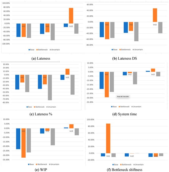
Figure 3.
Simulation results with uncertain and bottleneck. (a): Lateness; (b): Standard Deviation of the Lateness; (c): percentage of parts in lateness; (d): throughput time of the manufacturing system; (e): Work In Process; (f): Bottleneck shiftness.
The proposed method works better under the uncertain processing time of the machine in every case of utilization. The introduction of the bottleneck reduces the improvement of the proposed method when the utilization is medium and in some cases is worst with lower utilization.
These results show the robustness of the proposed method when the utilization of the manufacturing system is higher, while in case of lower utilization some conditions such as the introduction of the bottleneck can reduce significantly the performance.
Table 2 reports the couple of the α and β values that lead to a better result for each case tested.
Table 2.
Best values of α and β for the simulation cases.
The utilisation, power, bottleneck and processing time uncertain lead to different values of the weights. As the reader can notice, when the power available is lower, the workload of the parts in the queue (β) has minor importance. Otherwise, the workload of the parts in the queue is more important when the power available is higher or a machine is a bottleneck. The processing time uncertain leads to obtain the same importance between the two workloads evaluated.
6. Conclusions and Future Development Paths
This paper presents a method to allocate power among the machines of a flexible manufacturing system. Each machine processes the job with the processing time that depends on the power allocated. The method proposed used the Gale–Shapley algorithm, which is a game theory method to share resources. This decision model also works with limited computational time when the manufacturing system consists of several machines. The objective is a method that allows reducing the peak power needed to pursue a performance level.
In response to the first research question: What is the impact of the cooperation model based on the Gale-Shapley on the performance of a job shop manufacturing system? Using the simulation, the results show how the proposed method can support power allocation and improve performance measures. The medium or high average utilization and potential uncertainty in processing time improve the performance of the proposed method, while the bottleneck can reduce the effect of the proposed method. In response to the second research question: Can the peak power load reduce without a negative effect on the performance of the manufacturing system? The simulation results show that the same level of performance can be obtained with lower power available for the manufacturing system.
6.1. Managerial Implication
The study proposed in this paper evaluates the impact of the power allocation on the performance of a flexible manufacturing system considering the impact on the processing time. The results of this research suggest how the proposed method can support the manufacturing system on power allocation management. This is important, for example, if a renewable energy source is available to integrate into the manufacturing system. The proposed method can improve the use of renewable energy without reducing performance in case of demand fluctuations or uncertain processing time. Moreover, the proposed method can easily include other components of the industrial plant that need power allocation. The open innovation models can support the proposed model in the case of networks in SMEs that cooperate, sharing manufacturing resources.
6.2. Limitation and Future Research
This limitation of the research concerns the evaluation of the impact of the costs both in terms of peak power and production due to the change in the cutting speed. The cutting speed impacts the tool life of the manufacturing operations and the costs. Future research is needed to include the costs of energy in the manufacturing operations to evaluate the impact on the global costs. Moreover, the model proposed will include the introduction of a renewable energy source.
Funding
This research received no external funding.
Conflicts of Interest
The authors declare no conflict of interest.
Appendix A
| Vt [m/min] | Processing Time [min] | MRR [cm3/sec] | SEC [Kj/cm3] | Power [KJ/sec] | Energy [Kj] | |
| Pmin | 45 | 3.488888889 | 0.71656051 | 4.70108889 | 4.10861465 | 860.07 |
| 50 | 3.14 | 0.796178344 | 4.51548 | 4.335127389 | 816.738 | |
| 55 | 2.854545455 | 0.875796178 | 4.36361818 | 4.561640127 | 781.284545 | |
| 60 | 2.616666667 | 0.955414013 | 4.23706667 | 4.788152866 | 751.74 | |
| 65 | 2.415384615 | 1.035031847 | 4.12998462 | 5.014665605 | 726.740769 | |
| 70 | 2.242857143 | 1.114649682 | 4.0382 | 5.241178344 | 705.312857 | |
| 75 | 2.093333333 | 1.194267516 | 3.95865333 | 5.467691083 | 686.742 | |
| 80 | 1.9625 | 1.27388535 | 3.88905 | 5.694203822 | 670.4925 | |
| 85 | 1.847058824 | 1.353503185 | 3.82763529 | 5.920716561 | 656.154706 | |
| 90 | 1.744444444 | 1.433121019 | 3.77304444 | 6.147229299 | 643.41 | |
| 95 | 1.652631579 | 1.512738854 | 3.7242 | 6.373742038 | 632.006842 | |
| 100 | 1.57 | 1.592356688 | 3.68024 | 6.600254777 | 621.744 | |
| 105 | 1.495238095 | 1.671974522 | 3.64046667 | 6.826767516 | 612.458571 | |
| 110 | 1.427272727 | 1.751592357 | 3.60430909 | 7.053280255 | 604.017273 | |
| 115 | 1.365217391 | 1.831210191 | 3.57129565 | 7.279792994 | 596.31 | |
| 120 | 1.308333333 | 1.910828025 | 3.54103333 | 7.506305732 | 589.245 | |
| 125 | 1.256 | 1.99044586 | 3.513192 | 7.732818471 | 582.7452 | |
| 130 | 1.207692308 | 2.070063694 | 3.48749231 | 7.95933121 | 576.745385 | |
| 135 | 1.162962963 | 2.149681529 | 3.4636963 | 8.185843949 | 571.19 | |
| 140 | 1.121428571 | 2.229299363 | 3.4416 | 8.412356688 | 566.031429 | |
| 145 | 1.082758621 | 2.308917197 | 3.42102759 | 8.638869427 | 561.228621 | |
| 150 | 1.046666667 | 2.388535032 | 3.40182667 | 8.865382166 | 556.746 | |
| Pmax | 155 | 1.012903226 | 2.468152866 | 3.38386452 | 9.091894904 | 552.552581 |
| 160 | 0.98125 | 2.547770701 | 3.367025 | 9.318407643 | 548.62125 | |
| Average processing time | 2.235069444 | |||||
References
- Council of the European Union. Energy and Climate Change—Elements of the Final Compromise; Council of the European Union: Brussels, Belgium, December 2008; Volume 2008, pp. 1–18.
- USEIA. EIA—International Energy Outlook 2016: Chapter 7. Industrial Sector Energy Consumption; DOE/EIA-0484(2016); USEIA: Washington, DC, USA, August 2016.
- USEIA. EIA—Annual Energy Outlook 2016; DOE/EIA-0383(2016); USEIA: Washington, DC, USA, August 2016.
- Eurostat. Consumption of Energy—Statistics Explained. 2017. Available online: http://ec.europa.eu/eurostat/statisticsexplained/index.php/Consumption_of_energy (accessed on 17 January 2019).
- Faruqui, A.; Hledik, R.; Newell, S.A.; Pfeifenberger, J.P. The Power of Five Percent: How Dynamic Pricing Can Save $35 Billion in Electricity Costs; The Brattle Group: Cambridge, MA, USA, 2007; Available online: http://www.brattle.com/_documents/UploadLibrary/Upload574.pdf (accessed on 25 March 2019).
- Renna, P. Energy saving by switch-off policy in a pull-controlled production line. Sustain. Prod. Consum. 2018, 16, 25–32. [Google Scholar] [CrossRef]
- Frigerio, N.; Matta, A. Analysis on energy efficient switching of machine tool with stochastic arrivals and buffer information. IEEE Trans. Autom. Sci. Eng. 2016, 13, 238–246. [Google Scholar] [CrossRef]
- Beier, J. Existing Approaches in the Field of Energy Flexible Manufacturing Systems. In Sustainable Production, Life Cycle Engineering and Management; Springer: Cham, Switzerland, 2017. [Google Scholar]
- Abikarram, J.B.; McConky, K. Real time machine coordination for instantaneous load smoothing and photovoltaic intermittency mitigation. J. Clean. Prod. 2017, 142, 1406–1416. [Google Scholar] [CrossRef]
- Kim, H.-M.; Lim, Y.; Kinoshita, T. An Intelligent Multiagent System for Autonomous Microgrid Operation. Energies 2012, 5, 3347–3362. [Google Scholar] [CrossRef]
- Molina, T.; Gafurov, T.; Prodanovic, M. Proactive Control for Energy Systems in Smart Buildings. In Proceedings of the 2nd IEEE PES International Conference and Exhibition on Innovative Smart Grid Technologies (ISGT Europe), Manchester, UK, 5–7 December 2011; pp. 1–8. [Google Scholar]
- Dai, M.; Tang, D.; Giret, A.; Salido, M.A.; Li, W.D. Energy-efficient scheduling for a flexible flow shop using an improved genetic-simulated annealing algorithm. Robot. Comput. Int. Manuf. 2013, 29, 418–429. [Google Scholar] [CrossRef]
- Gajic, D.; Hadera, H.; Onofri, L.; Harjunkoski, I.; Di Gennaro, S. Implementation of an integrated production and electricity optimization system in melt shop. J. Clean. Prod. 2017, 155, 39–46. [Google Scholar] [CrossRef]
- Chen, T.-L.; Cheng, C.-Y.; Chou, Y.-H. Multi-objective genetic algorithm for energy-efficient hybrid flow shop scheduling with lot streaming. Ann. Oper. Res. 2018. [Google Scholar] [CrossRef]
- Shim, S.-O.; Park, K.; Choi, S. Sustainable Production Scheduling in Open Innovation Perspective under the Fourth Industrial Revolution. J. Open Innov. Technol. Mark. Complex. 2018, 4, 42. [Google Scholar] [CrossRef]
- Chesbrough, H.W. Open Innovation: The New Imperative for Creating and Profiting from Technology; Harvard Business Press: Boston, MA, USA, 2003. [Google Scholar]
- Hoogeveen, H. Multicriteria scheduling. Eur. J. Oper. Res. 2005, 167, 592–623. [Google Scholar] [CrossRef]
- Liu, Y.; Dong, H.; Lohse, N.; Petrovic, S.; Gindy, N. An investigation into minimizing total energy consumption and total weighted tardiness in job shop. J. Clean. Prod. 2014, 65, 87–96. [Google Scholar] [CrossRef]
- Yan, H.; Fei, L.; Hua-jun, C.; Cong-bo, L. A bi-objective model for job-shop scheduling problem to minimize both energy consumption and makespan. J. Cent. South Univ. Technol. 2005, 12, 167–171. [Google Scholar]
- Módos, I.; Šůcha, P.; Hanzálek, Z. Algorithms for Robust Production Scheduling with Energy Consumption Limits. Comput. Ind. Eng. 2017, 112, 391–408. [Google Scholar] [CrossRef]
- Sun, Z.; Li, L. Potential capability estimation for real time electricity demand response of sustainable manufacturing systems using Markov decision process. J. Clean. Prod. 2014, 65, 184–193. [Google Scholar] [CrossRef]
- Fernandez, M.; Li, L.; Sun, Z. Just-for-peak buffer inventory for peak electricity demand reduction of manufacturing systems. Int. J. Prod. Econ. 2013, 146, 178–184. [Google Scholar] [CrossRef]
- Sun, Z.; Li, L.; Fernandez, M.; Wang, J. Inventory control for peak electricity demand reduction of manufacturing systems considering the tradeoff between production loss and energy savings. J. Clean. Prod. 2014, 82, 84–93. [Google Scholar] [CrossRef]
- Nagasawa, K.; Ikeda, Y.; Irohara, T. Robust flow shop scheduling with random processing times for reduction of peak power consumption. Simul. Model. Pract. Theory 2015, 59, 102–111. [Google Scholar] [CrossRef]
- Wang, J.J.; Wang, L. Decoding methods for the flow shop scheduling with peak power consumption constraints. Int. J. Prod. Res. 2019. [Google Scholar] [CrossRef]
- Beier, J.; Thiede, S.; Herrmann, C. Energy flexibility of manufacturing systems for variable renewable energy supply integration: Real-time control method and simulation. J. Clean. Prod. 2017, 141, 648–661. [Google Scholar] [CrossRef]
- Popp, R.S.H.; Zaeh, M.F. Determination of the technical energy flexibility of production systems. Adv. Mater. Res. 2014, 1018, 197–202. [Google Scholar] [CrossRef]
- Schultz, C.; Sellmaier, P.; Reinhart, G. An approach for energy-oriented production control using energy flexibility. Procedia CIRP 2015, 29, 197–202. [Google Scholar] [CrossRef]
- Zhang, Z.-C.; Hong, W.-C.; Li, J. Electric load forecasting by hybrid self-recurrent support vector regression model with variational mode decomposition and improved cuckoo search algorithm. IEEE Access 2020, 8, 14642–14658. [Google Scholar] [CrossRef]
- Hong, W.-C.; Li, M.W.; Geng, J.; Zhang, Y. Novel chaotic bat algorithm for forecasting complex motion of floating platforms. Appl. Math. Model. 2019, 72, 425–443. [Google Scholar] [CrossRef]
- Zhang, Z.-C.; Hong, W.-C. Electric load forecasting by complete ensemble empirical model decomposition adaptive noise and support vector regression with quantum-based dragonfly algorithm. Nonlinear Dyn. 2019, 98, 1107–1136. [Google Scholar] [CrossRef]
- Dong, Y.; Zhang, Z.; Hong, W.-C. A hybrid seasonal mechanism with a chaotic cuckoo search algorithm with a support vector regression model for electric load forecasting. Energies 2018, 11, 1009. [Google Scholar] [CrossRef]
- Hong, W.-C.; Dong, Y.; Lai, C.-Y.; Chen, L.-Y.; Wei, S.-Y. SVR with hybrid chaotic immune algorithm for seasonal load demand forecasting. Energies 2011, 4, 960–977. [Google Scholar] [CrossRef]
- Jalal, A.Q.; Allalaq, H.A.E.; Shinkevich, A.I.; Kudryavtseva, S.S.; Ershova, I.G. Assessment of the Efficiency of Energy and Resource-saving Technologies in Open Innovation and Production Systems. Int. J. Energy Econ. Policy 2019, 9, 289–296. [Google Scholar] [CrossRef]
- Kudryavtseva, S.S.; Shinkevich, A.I.; Shvetsov, M.Y.; Bordonskaya, L.A.; Gorlachev, V.P.; Persidskaya, A.E.; Schepkina, N.K. National open innovation systems: An evaluation methodology. J. Sustain. Dev. 2015, 6, 270–278. [Google Scholar] [CrossRef]
- Lee, S.; Park, G.; Yoon, B.; Park, J. Open innovation in SMEs—An intermediated network model. Res. Policy 2010, 39, 290–300. [Google Scholar] [CrossRef]
- Hossain, M.; Kauranen, I. Open innovation in SMEs: A systematic literature review. J. Strategy Manag. 2016, 9, 58–73. [Google Scholar] [CrossRef]
- Shim, S.-O.; Park, K. Technology for Production Scheduling of Jobs for Open Innovation and Sustainability with Fixed Processing Property on Parallel Machines. Sustainability 2016, 8, 904. [Google Scholar] [CrossRef]
- Yusr, M.M. Innovation capability and its role in enhancing the relationship between TQM practices and innovation performance. J. Open Innov. Technol. Mark. Complex. 2016, 2, 6. [Google Scholar] [CrossRef]
- Park, H.S. Technology convergence, open innovation, and dynamic economy. J. Open Innov. Technol. Mark. Complex. 2017, 3, 24. [Google Scholar] [CrossRef]
- Yun, J.J.; Won, D.; Park, K. Dynamics from open innovation to evolutionary change. J. Open Innov. Technol. Mark. Complex. 2016, 2, 7. [Google Scholar] [CrossRef]
- Lichtenthaler, U.; Lichtenthaler, E. A capability-based framework for open innovation: Complementing absorptive capacity. J. Manag. Stud. 2009, 46, 1315–1338. [Google Scholar] [CrossRef]
- Argoneto, P.; Renna, P. Capacity sharing in a network of enterprises using the Gale–Shapley model. Int. J. Adv. Manuf. Technol. 2013, 69, 1907–1916. [Google Scholar] [CrossRef]
- Renna, P. Decision-making method of reconfigurable manufacturing systems’ reconfiguration by a Gale-Shapley model. J. Manuf. Syst. 2017, 45, 149–158. [Google Scholar] [CrossRef]
- Renna, P. Workload control policies under continuous order release. Prod. Eng. Res. 2015, 9, 655–664. [Google Scholar] [CrossRef]
- Kara, S.; Li, W. Unit process energy consumption models for material removal processes. CIRP Ann. Manuf. Technol. 2011, 60, 37–40. [Google Scholar] [CrossRef]
- Anderberg, S.; Kara, S.; Beno, T. Impact of Energy Efficiency on Computer Numerically Controlled Machining. Proc. Inst. Mech. Eng. Part B J. Eng. Manuf. 2009, 224, 531–541. [Google Scholar] [CrossRef]
- Gale, D.; Shapley, L.S. College admissions and the stability of marriage. Am. Math. Mon. 1962, 69, 9–14. [Google Scholar] [CrossRef]
- Kobayashi, H.; Matsui, T. Creating Strategies for the Gale-Shapley Algorithm with Complete Preference Lists. Algorithmica 2010, 58, 151–169. [Google Scholar] [CrossRef]
- Teo, C.-P.; Sethuraman, J.; Tan, W.-P. Gale-Shapley stable marriage problem revisited: Strategic issues and applications. Manag. Sci. 2001, 47, 1252–1267. [Google Scholar] [CrossRef]
- Huang, Z.; Kim, J.; Sadri, A.; Dowey, S.; Dargusch, M.S. Industry 4.0: Development of a multi-agent system for dynamic value stream mapping in SMEs. J. Manuf. Syst. 2019, 52, 1–12. [Google Scholar] [CrossRef]
- Lawrence, S.R.; Buss, A.H. Shifting Production Bottlenecks: Causes, Cures, and Conundrums. Prod. Oper. Manag. 1994, 3, 21–37. [Google Scholar] [CrossRef]


© 2020 by the author. Licensee MDPI, Basel, Switzerland. This article is an open access article distributed under the terms and conditions of the Creative Commons Attribution (CC BY) license (http://creativecommons.org/licenses/by/4.0/).