Solving a Special Case of the Generalized Assignment Problem Using the Modified Differential Evolution Algorithms: A Case Study in Sugarcane Harvesting

Abstract

We proposed and created a methodology to solve a real-world problem, which is a special case of the generalized assignment problem. The problem consists of assigning drivers to harvesters, which will then be assigned to harvest sugarcane in order to maximize daily profit. A set of drivers have various levels of experience. Therefore, a different capability to harvest sugarcane leads to a range of daily wages. Each harvester has different operating years and engine size, which affects its fuel consumption rate and capacity to harvest sugarcane, respectively. Assigning a worker to a harvester can improve the fuel consumption and efficiency of the harvester. We developed a mathematical model to reflect this problem and to solve it to find the maximum outcome using Lingo v.11 commercial optimization software. Since Lingo v.11 is limited to solving only small-size test instances, for medium to large test instances, four modified differential evolution (MDE) algorithms were used to solve the problem: MDE-1, MDE-2, MDE-3, and MDE-4. MDE-2 was found to be the best proposed heuristics because it has intensification and diversification ability. MDE has been tested with the case study. We tried to increase the daily profit by implementing three strategies: (1) change all harvesters that are more than five years old, (2) train drivers to reach maximum capacity, and (3) a combination of 1 and 2. Each strategy has a different investment. The breakeven point (number of days) to return the investment was calculated from the increase of daily profit. The computational results show that strategy 2 is the best because it has the quickest rate of investment return rate. However, this strategy has a disadvantage, since it is possible that drivers may leave the company if they have been highly trained. Moreover, strategy 1 has an acceptable break-even point at 392 days.

1. Introduction

Sugarcane is a globally important commercial crop that can be used to produce both direct and indirect products such as sugar, ethanol, jaggery, and fodder. Sugarcane is a tall perennial grass reaching 3 to 4 m in height. Therefore, its cultivation is not easy, and it needs special tools to be harvested effectively.

To harvest sugarcane, cutting at the ground level is needed because the sweetness level is higher in this part of the cane. The tips of the stem and leaves are immediately removed. Traditionally, hand harvesting is effective to harvest sugarcane. Currently, mechanical harvesters play an important role in sugarcane harvesting due to a shortage of labor and increased labor costs. A harvester is very powerful since it can replace 200 laborers. In the first era of using the harvester instead of human labor, the price of the harvester is still high. The mumber of harvesters in use is limited but there are many farmers who want to use it. Therefore, the scheduling of fields to be harvested by the harvesters is needed to achieve the aim of the farmers or the owner of the harvester. The scheduling problem is one out of the most famous combinatorial optimization for all researchers. There are some excellent examples of the studies involved in the scheduling problem such as Shim, et al. [1], Shim and Park [2], Jeong, et al. [3], Joo, et al. [4], and Jeong and Shim [5].

Later on, many brands, sizes, and types of the harvester have been released to the market. There is limitation for using a particular harvester such as some fields cannot be served by some harvester types due to the steepness of the field or insufficient roads/tracks to the field. This make it more difficult to assign the field to the suitable harvester. Moreover, the cost control is also of interest to the owner of the harvester. The level of effectiveness of the machine has been considered when assigning the harvester to the field. It depends on a few factors, such as the model and number of operating years, and the experience of the user. In this research study, these variations have been taken into account in order to generate fair results.

This research aims to assign harvesters to harvest sugar in sugarcane fields. One harvester can be assigned to more than one field if it has enough time remaining. Different harvesters use different amounts of time because they have different harvesting capacities. The harvester has limited working time. Therefore, this problem falls into behavior according to the generalized assignment problem (GAP). The field presents the task and the harvester can be interpreted as the agent in the GAP problem.

A generalized assignment problem (GAP) is where the task is assigned to one employee or agent. The agent can serve more than one task and different assignments consume different resources. The agent must use less resource than its capacity. GAP was first proposed by Ross and Soland [6], and proved to be an NP-hard problem [7]. Later, Chu and Beasley [8] proved that GAP is NP-complete and the existing exact methods are practical only for instances where there are no additional constraints.

An extended version has been studied, so that the GAP can imitate the behavior of a real-world problem. Osorio and Laguna [9] took into consideration the availability of workers and the possibility of job rotation in the worker assignment problem. Alfares [10] and Elshafei and Alfares [11] discussed the restrictions on working days and off-days for workers. Alfares [10] tried to optimize the number of workers, while Elshafei and Alfares [11] tried to minimize the labor cost. Recently, location/allocation has been considered while making decisions in GAP [12]. The proposed problem that is closest to the GAP type is the multilevel GAP, which was introduced by Laguna et al. 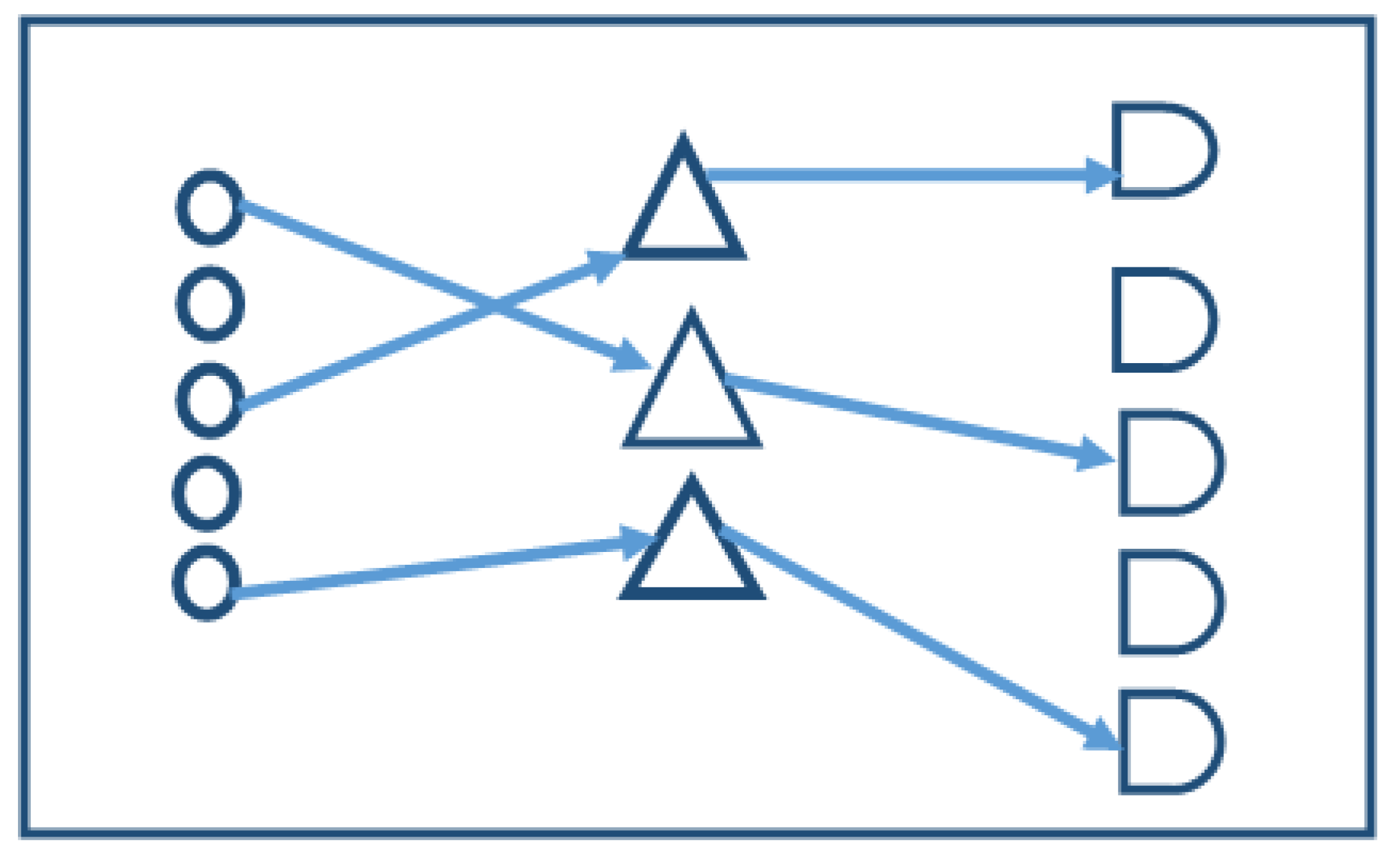[13]. We assigned the driver to the harvester. The skill level of the worker will affect the effectiveness of the harvester, which also has a different capacity. The capacity of the harvester means the driving and harvest speed affect its resource usage. Then the fields will be assigned to the harvester, and this assignment affects the profit because each field has different sweet and density levels, which affect the amount of sugarcane that can be harvested per day. The harvester can be assigned to serve more than one field if it has enough daily capacity (time). Therefore, the proposed problem is the special case of GAP where many new parameters and conditions have been added to the problem definition.

Comparing our problem to Kaewman et al. [14], this article proposes the multi-level assignment problem. The young chicken farm has been assigned to deliver the chicken to the egg farm (to feed the young chicken and collect the eggs from it to sell). The number of chickens that is needed in the egg farm has to be at least 50% satisfied and it can be obtained from more than one chicken farm. When finishing the assignment of the chicken farm to deliver chickens to the egg farms, a suitable truck will be assigned to transport the chicken from the chicken farm to the egg farm. In the real world, the trucks have different ages of use or machine type, which can consume different fuel usage. Moreover, the experience and driving style of a specific driver is also to change the fuel consumption (speed used), which can change the total profit generated. The special attributes addressed above have been considered in our study.

The proposed problem is one out of the combinatorial optimization, which is hard to solve. Most of the small sizes of the test instances have been solved by the exact methods while larger sizes of test instances and the exact methods are mostly unable to solve the problems into optimality within the reasonable computational time. The metaheuristics and heuristics are used to find the promising solution. Metaheuristics have been successfully developed to solve various problem types both in discrete and continuous optimization such as disease detection from medical images [15], fruit peel defects detection [16], develop the intelligent simulation and control model of electric drive engine [17], and use to solve the GAP problem [18]. Solving GAP, some effective exact methods have been proposed to solve classical GAP, such as branch and bound [6], branch and price [19], etc. To reduce the computational time of the exact method where the problem size is very large, heuristics and metaheuristics have been presented to solve the GAP and other combinatorial optimization problems such as the heuristics approximation method [20] and the approximation approach to adapt the knapsack solving method [21], heuristics, where it is the combination of the exact method and heuristics [22], simulated annealing [23], tabu search [24], genetic algorithm [25], very-large-scale neighborhood search [26], bee algorithm [27], and differential evolution algorithm (DE) to solve the GAP has been proposed by Tasgetiren et al. [28] and Sethanan and Pitakaso [29]. The computational results show that DE outperforms all other heuristics proposed so far.

DE has been used to solve various types of problems such as production planning [30,31], manufacturing problems [32], and more. Dechampai et al. [33] presented DE to solve the capacitated vehicle routing problem (VRP) in the poultry industry with the flexibility of mixing pickup and delivery services and maximum duration of a route. Akkararungruangkul and Kaewman [32] studied the special case of a vehicle routing problem where the condition of the road was considered. They modified the mutation process by using different formulas to increase the search capacity of DE, and the computational result showed that the new formula outperformed the traditional formula of DE. Sethanan and Pitakaso [34] improved DE by adding two more steps known as reincarnation and the survival process to improve the intensification search of the DE. These steps were added after the selection process. Sethanan and Pitakaso [29] improved the differential evolution algorithm by adding effective local searches to increase the search mechanism for solving a generalized assignment problem. With the use of different mutation and recombination processes and matching to improve the solution quality, it has been proven that using different pairs of mutation and recombination processes gives a different solution quality, such as in Pitakaso and Sethanan [29] and Boon, et al. [35].

From the literature, DE is more effective if the local search is included, but it increases the computational time. DE is modified by adding more processes to the original version, such as the recombination process, the reborn process, and the reincarnation process, to get better solutions. These processes can improve the solution quality of the original DE because they enhance the search capability of the original system.

Therefore, DE is designed to solve the proposed problem. The mutation process is modified to include two more sets of vectors (best vector and random vector) that are used in addition to the set of target vectors, which is used in the original version of DE. The selection of these three sets of vectors was done by probability, which can increase or decrease during the simulation. This one controls by the score of each set of vectors. The score was updated regarding the quality of the solution via that set of vectors. Moreover, three sets of vectors were introduced into the original DE mechanism. These sets of vectors are categorized as best vector (BV), second best vector (B2), and randomly selected vector (RS). These three vectors were stored in the selection process and the local search (swap) was applied to them.

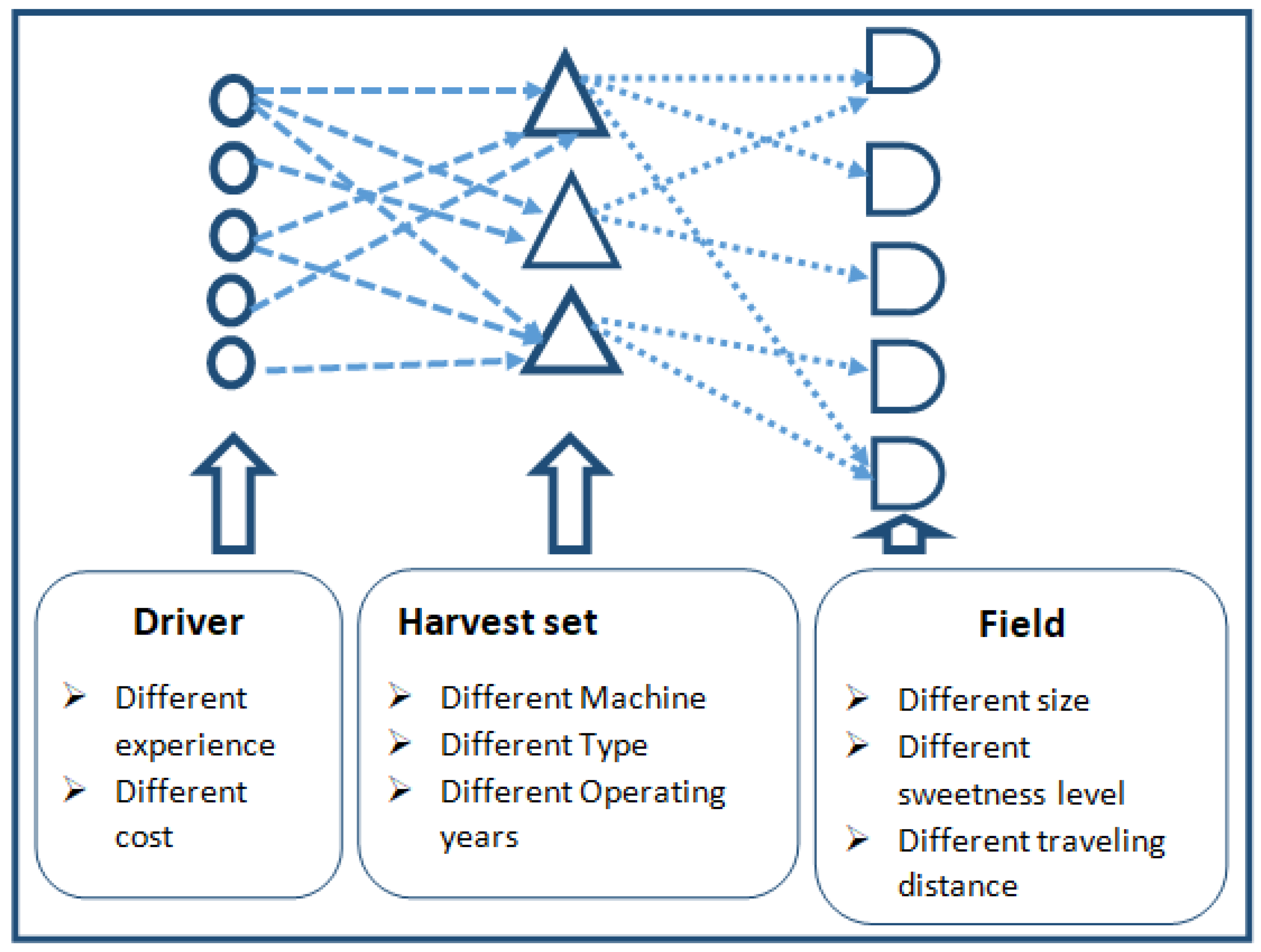
The contributions of this paper are two-fold: (1) the real-world problem, which is the special case of the GAP that has been introduced, and (2) the modified differential evolution. The real-world problem is a special case of GAP, since it has four attributes, which is more than any other GAP proposed in the literature. The attributes are: (1) drivers have different levels of experience, (2) each harvester has different capacity and operating years, which results in different effectiveness in harvesting, (3) the time required to harvest each field depends on the harvester used and its driver, and (4) the profit from harvesting depends on the sweetness of the sugarcane, which is dependent on the field. These attributes have to be accounted to the model so that the profit of the whole system is maximized.

This paper has been organized as follows: Section 2 describes the mathematical model that represents the proposed problem. Section 3 describes the proposed method that was used to solve the problem (DE). Section 4 gives the computational framework and results. Lastly, Section 5 is the conclusion and future outlook.

2. Problem Definition and Mathematical Model for Special Case of the Generalized Assignment Problem

This section explains the problem definition and the mathematical model that represents the proposed problem.

2.1. Problem Definition

We call our problem a special case of the generalized assignment problem in this particular research study. The proposed problem is composed of three actors: (1) the driver, (2) the harvester set, and (3) the sugarcane field. The problem is to pair a driver with a suitable harvester set to harvest a suitable sugarcane field so that the daily profit is maximized. The profit depends on the income and cost generated in the system, while the income is generated from the amount of harvested sugarcane sold multiplied by the sweetness level of the harvested sugarcane (the price of sugarcane sold is based on per ton unit). The profit is the result of total income subtracted by the cost of the harvester’s fuel consumption and the corresponding driver’s daily wages. There is a pool of drivers with various levels of experience and wages. The harvester sets have a range of machine types and operating years, which determines the fuel consumption rate. The efficiency of harvesting is also affected by the driver of the particular harvester set. After the harvester set and its driver have been assigned, they will start to harvest the assigned sugarcane field, where each plant has a different size, sweetness level, and travelling distance. All of these activities generate the special case of GAP (S-GAP). The framework of the unsolved and solved problem is shown in Figure 1.

As illustrated in Figure 1 and Figure 2, the solved problem is that one driver will be paired with a suitable harvester set to harvest a suitable sugarcane field. The mathematical model of the proposed problem is shown in Section 2.2.

2.2. Mathematical Model

The mathematical model for economic crop planning is as follows:

Indices

i

Workers i when i = 1, …, I

j

Harvester j when j = 1, …, J

k

Sugarcane field k when k = 1, …, K

Parameters

I

Number of available workers

J

Number of available harvesters

K

Number of sugarcane fields

D_jk

Hours required to travel from the harvester parking area j to the sugarcane field k

P_i

Experience factor of worker i (effective in the cutting factor)

R_i

Experience factor in using fuel of worker j

E_j

Fuel consumption rate of harvester j (baht/hours)

U_jj

Scaling factor of using fuel depending on years that the harvester has been used

V

Production rate of sugarcane (tons/rai)

B_k

Sweetness factor of sugarcane field k

S_k

Selling price of sugarcane field k (baht)

A_k

Area of sugarcane field k (rai)

C_i

Hiring cost of worker i (baht/day)

T_j

Theoretical cutting speed of harvester j (rai/hour)

L

Work regulation of worker (hours/day)

Decision Variables

• X_jk $=\{\begin{array}{c} 1 if cutting set j is assigned to sugarcane field k\\ 0 otherwise\end{array}$
• Y_ij $=\{\begin{array}{c} 1 if worker i is assigned to cutting set j\\ 0 otherwise\end{array}$
• $\mathrm{Wi}=\{\begin{array}{c} 1 if worker i is in used\\ 0 otherwise\end{array}$
• Z_k $=\{\begin{array}{c} 1 if sugarcane field is assigned by at least one cutting set\\ 0 otherwise\end{array}$
• H_jk = Hours required to cut sugarcane in field k using harvester j
• Q_jk = Hours required to travel from j to k
• M_j = Real fuel consumption rate of harvester j (baht/hours)
• N_j = Real cutting speed of harvester j (rai/hours)

Objective function

$$\max z={\displaystyle \sum }_{k=1}^K{Z}_k\times B_k\times S_k-{\displaystyle \sum }_{k=1}^K{\displaystyle \sum }_{j=1}^J{X}_{jk}\times D_{jk}\times M_j-{\displaystyle \sum }_{k=1}^K{\displaystyle \sum }_{j=1}^J{H}_{jk}\times X_{jk}\times M_j-{\displaystyle \sum }_{k=1}^K{W}_i\times C_i$$

(1)

Subjected to

$$Z_k\le {{\displaystyle \sum }}_{j=1}^J{X}_{jk}\forall k=1\dots K$$

(2)

$${{\displaystyle \sum }}_{k=1}^K{X}_{jk}\le 1\forall j=1\dots J$$

(3)

$${{\displaystyle \sum }}_{j=1}^J{Y}_{ij}\le 1\forall i=1\dots I$$

(4)

$$W_i\ge {{\displaystyle \sum }}_{j=1}^J{Y}_{ij}\forall i=1\dots I$$

(5)

$$M_j={{\displaystyle \sum }}_{i=1}^I{Y}_{ij}\times R_i\times E_j\times U_j\forall j=1\dots J$$

(6)

$$N_j={{\displaystyle \sum }}_{i=1}^I{Y}_{ij}\times T_J\times P_i\forall j=1\dots J$$

(7)

$$\begin{gathered} {\mathrm{Q}}_{\mathrm{jk}}=2\times {\mathrm{D}}_{\mathrm{jk}}\forall k=1\dots K \\ \forall j=1\dots J \end{gathered}$$

(8)

$$\begin{gathered} {\mathrm{H}}_{\mathrm{jk}}=\frac{{\mathrm{A}}_{\mathrm{k}}}{{\mathrm{N}}_{\mathrm{j}}}k=1\dots K \\ \forall j=1\dots J \end{gathered}$$

(9)

$${{\displaystyle \sum }}_{\mathrm{i}=1}^{\mathrm{I}}{\mathrm{Q}}_{\mathrm{JK}}\times {\mathrm{H}}_{\mathrm{JK}}\times {\mathrm{X}}_{\mathrm{JK}}\le \mathrm{L}\forall j=1\dots J$$

(10)

$$\begin{gathered} X_{jk}\ge {{\displaystyle \sum }}_{i=1}^I{Y}_{ij}k=1\dots K \\ \forall j=1\dots J \end{gathered}$$

(11)

The objective of Equation (1) is to maximize profit from selling sugarcane, which is related to the function of sugarcane sweetness. The actual profit is generated by subtracting the transportation cost, fuel cost to operate the harvester set, and labor cost from income from mathematical model. Regarding Equation (2), it is important that only sugarcane field k, which has been assigned harvester set j, is harvested. Regarding Equation (3), we need to ensure that one harvester set is assigned to only one field at a time. Equations (4) and (5) address the assignment of one worker to one harvester set at a time. Equation (6) is used to calculate the real fuel consumption if we assign worker I to harvester set j. Equation (7) is used to calculate the real cutting speed of harvester set j, which is the function of the efficiency of the worker who has been assigned to the harvester set. Equation (8) specifies the traveling time from j to k. Equation (9) is the number of hours required to harvest sugarcane at field k, Equation (10) ensures that the time used to travel and harvest is not over the allowed working hours per day, and Equation (11) ensures that only the harvester set with an assigned driver will be allowed to harvest in field k.

3. Proposed Heuristic

We present a differential evolution algorithm (DE) to solve the proposed problem. Originally, the DE is composed of four steps: (1) generate initial solution, (2) implement the mutation process, (3) execute the recombination process, and (4) complete the selection process. The modified DE that is discussed in this paper has five steps: (1) generate initial solution, (2) implement the mutation process, (3) execute the recombination process, (4) perform the selection process, and (5) update the reserved vectors.

Generally, DE has three types of vectors: (1) target vector, (2) mutant vector, and (3) trial vector. The modified DE (MDE) presented in this paper adds the following vectors:

(1) Set of second best vectors (B2-vectors)

The second best vector is stored while the selection process is performed. The other worse solution while comparing to the objective function is deleted from the system, but only the second best vector set is kept. This set is composed of the second best vector of all vectors and is iteratively updated. This increases the intensification of the algorithm because we will search intensively on these vectors when the predefined condition is met.

(2) Set of randomly selected vectors (RS-vectors)

The RS-vector is selected from the worse solution while the selection process is performed. The worse vector normally is updated in the set of second best vectors, and then the old second best vector is deleted. When it is deleted, the RS-vector is updated. There are two choices to deal with the old second best vector: (1) delete it from the system, or (2) store it as an RS-vector. The probability is controlled by using Equation (13).

(3) Set of vectors that are iteratively randomly generated (RV-vectors).

(4) Best vector given by all vectors in all previous iterations (BV-vectors).

Please note that RS-vectors, RV-vectors, B2-vectors, and BV-vectors have the same number of vectors as target vectors, mutant vectors, and trial vectors.

Originally, mutant vectors come only from operating the target vector, while mutant MDE vectors come from operating target vectors, BV-vectors, and RV-vectors. This is used to increase intensification of the original DE, but it also has a chance to select from the set of random vectors that can still give good diversification of the DE. The chance depends on the current iteration. If it is in the very first iteration of the probability, then, to select from the random vector, is higher than the very last iteration.

Moreover, the swap heuristics is performed in the sets of BV-vectors, RS-vectors, and B2-vectors. The following steps are used to explain the modified differential evolution algorithm (MDE).

3.1. Generating the Initial Solution and Decoding Method

The Differential evolution algorithm (DE) generally works on real numbers because the mutation and recombination processes are about using arithmetic signs to calculate mutant and trial vectors. This section explains how to get the solution to the problem from the real numbers generated from the DE’s operators.

3.1.1. Initial Solution

In the first iteration, the value in the position of each vector that has a size of 1 × D is randomly generated. D is the total number of sugarcane fields, harvesters, and drivers. For example, if we have six sugarcane fields, four harvester sets, and five drivers, D is equal to 6 + 4 + 5, which is 15. If NP = 5, this denotes NP as the number of vectors required. The initial target vectors are shown in

Table 1. Randomly generated target vectors in the first iteration.

Type	Sugarcane Field						Harvester				Driver
#Vector	1	2	3	4	5	6	1	2	3	4	1	2	3	4	5
1	0.84	0.39	0.92	0.56	0.06	0.72	0.72	0.09	0.43	0.47	0.65	0.36	0.63	0.00	0.32
2	0.71	0.45	0.40	0.63	0.78	0.07	0.61	0.16	0.54	0.12	0.56	0.70	0.71	0.70	0.38
3	0.55	0.20	0.63	0.34	0.39	0.14	0.10	0.93	0.61	0.09	0.06	0.35	0.88	0.92	0.06
4	0.80	0.75	0.49	0.76	0.74	0.55	0.18	0.82	0.90	0.57	0.75	0.44	0.86	0.19	0.94
5	0.22	0.20	0.12	0.42	0.74	0.90	0.72	0.09	0.43	0.47	0.65	0.36	0.63	0.00	0.32
Ak	80	50	40	70	32	41
Bk	1.2	1.5	0.9	0.8	1.0	0.8
Ej							120	180	110	130
Uj							1.1	1.3	1.0	1.2
Tj							9	10	6	8
Ri											1.2	0.7	0.8	1.1	1.2
Pi											0.9	1.2	1.1	0.9	0.8

A_k, area of field k (rai). B_k, sweetness factor of field k. E_j, fuel consumption rate of harvester j (baht/hours). U_j, used/aged factor of harvester j. T_j, harvest rate of harvester j (rai). R_i, experience factor affecting fuel consumption rate of driver i. Pi, experience level affecting the harvesting rate of driver i.

.

From Table 1, one vector is divided into three subsets. The first subset (first six positions) represents the sugarcane field, while the second (next four positions) and third (last five positions) subsets represent the harvester and driver, respectively. The information on an example that will be used to illustrate the proposed heuristics is given in Table 1 as well. More needed information is as follows: (1) fuel cost is 115 Thai baht (THB)/h, (2) selling price (S) of the sugarcane is 600 THB/ton, (3) standard sugar cane obtained from 1 rai of the sugarcane field is equal to 12 tons, (4) all drivers are only allowed to work a maximum of nine hours per day, and (5) the time required to drive from the parking area of each harvester set to each sugarcane field is shown in

Table 2. Time (h) required to drive from the parking area of harvester set j to field k.

Field	1	2	3	4	5	6
Harvester
1	0.80	0.08	0.99	0.35	0.89	0.15
2	0.32	0.79	0.11	0.04	0.18	0.55
3	0.84	0.65	0.66	0.70	0.08	0.05
4	0.25	0.95	0.08	0.63	0.89	0.21

.

3.1.2. Decoding Method

We designed our decoding method to have five steps, as follows.

(1)

Sort all subsets of vectors separately (field, harvester, and driver) in ascending order. The results of sorting are shown in

Table 3. Results of sorting value in the position of vector 1.

Type		Sugarcane Field							Harvester					Driver
Order		1	5	4	3	6	2		2	3	4	1		4	5	2	3	1
1		0.08	0.21	0.22	0.24	0.45	0.61		0.09	0.43	0.47	0.72		0.00	0.32	0.36	0.63	0.65

. The sugarcane field order is 1, 5, 4, 3, 6, and 2. The harvester order is 2, 3, 4, and 1 while the driver’s order is 4, 5, 2, 3, and 1, respectively.

(2)

Assign a driver to a harvester and assign the harvester to the sugarcane field(s) using the order obtained from step 1. We first assign the driver to the harvester. The pair of the driver and harvester will be assigned to serve the sugarcane field. The order of assignment will be executed according to the orders obtained from step 1. Two rules that have to be kept during the assignment is: (2.1) Assign the entity (field, harvester, driver) that is in position at the front of the order first and (2.2) if the current position violates the capacity constraints of the harvester (maximum time used 9 h.), the entity that is in the next position is allowed to be replaced.

For instance, when driver 4 (first position in driver’s order) is assigned to harvester set 2 (first order of harvester’s order), the real harvester rate after the harvester is calculated from the experience factor of worker i (P_i) multiplied by the standard harvesting rate of harvester j (T_j). Therefore, the real harvesting rate while we assign driver 4 to harvester 2 is 0.9 × 10 = 9 rai/h. Then we assign the pair of driver 4 and harvester 2 to sugarcane field 1 (first sugarcane field in the order). The traveling time from harvester set 2 to field 1 is 0.32 h (Table 2). If we have 9 h available, the traveling time used is 0.32. Therefore, it has 9 – (0.32 × 2) = 8.36 h left for harvester 2. As the result, a maximum of 75.24 rai can be harvested with this matchup, since the harvesting field 1 cannot be done within 8.36 h because field 1 has an area of 80 rai to be harvested, which means it needs 8.88 h to harvest. However, field 1 cannot be assigned to serve field 1. The next field’s order is field 5, which will be assigned to harvester 2 instead of field 1. Field 5 has an area of 34 rai. Harvester set 2 requires 4.13 h (traveling time from harvester set 2 to field 5 is 0.18 h). Hence, 4.87 harvesting hours are left. Therefore, we have to find another field from the list that is possible to support harvester set 2. Field 3 is the next field that is possible to assign harvester set 2. The results of the assignment are shown in

Table 4. Results from the assignment process.

Driver	Harvester	Maximum Cap. Rai/Hours	Field	Area (rai) (B)	Hours Required (B/A)
4	2	0.9 × 10 = 9	5	34	4.13
			3	40	4.607
5	3	0.8 × 6 = 4.8	6	41	8.64
2	4	1.2 × 8 = 9.6	1	80	8.83
3	1	1.1 × 9 = 9.9	4	70	7.77

.

(3) Calculate the profit generated from the assignment in step 2.

From Table 4, the fields that are harvested are 5, 3, 6, 1, and 4, which have an area of 34, 40, 41, 80, and 70 rai, respectively. These fields can produce 408, 480, 492, 960, and 840 tons of sugarcane, respectively (column A × 12 tons/rai). The sweetness factor (Sk) multiplied by the price of sugarcane per ton (600 THB/t) is used to get the real selling price of sugarcane produced from each field (see column D). Lastly, the real selling price multiplied by the amount of sugarcane in the field gives income (THB) for this specific assignment (

Table 5. Income of the harvesting plan.

Field	Total Area (A)	Amount of Sugarcane (ton) A × 12 (C)	Sweetness Factor (Sk) (B)	Real Selling Price (baht) (D) = 1500 × B	Income (baht) D × C
5	34	408	1	600	244,800
3	40	480	0.9	540	259,200
6	41	492	0.8	480	236,160
1	80	960	1.2	720	691,200
4	70	840	0.9	540	453,600

). The total income of this assignment is 1,884,960 baht.

Table 6. Results of calculating hours required to execute the plan.

Driver	Harvester	Field	Total Area (Ak) (A)	Harvesting Speed (Tj) (B)	Efficiency Factor of Worker (Pi) (C)	Real Harvesting Rate Nj = B × C (D)	Hours Required to Harvest Field k D = A/D	Traveling Time (Two-Way) (E)	Total Time Used F = D + E
4	2	5	34	10	0.9	9	3.78	0.36	4.14
		3	40	10	0.9	9	4.44	0.22	4.66
5	3	6	41	6	0.8	4.8	8.54	0.10	8.64
2	4	1	80	8	1.2	9.6	8.33	0.50	8.83
3	1	4	70	9	1.1	9.9	7.07	0.35	7.42

and

Table 7. Results of calculating the total cost for the plan.

Driver	Harvester	Engine Type (Uj) (A)	Theoretical Fuel Usage (Ej) (baht/hours) (B)	Experience Factor in Using Fuel (Ri) (C)	Real Fuel Usage Rate (Mj) D = A × B × C	Total Time Used (From Table 6) (E)	Total Fuel Cost F = E × D
4	2	1.3	180	1.1	257.4	4.14	1065.64
		1.3	180	1.1	257.4	4.66	1199.48
5	3	1.0	110	1.2	132	8.64	1140.48
2	4	1.2	130	0.7	109.2	8.83	964.24
3	1	1.1	120	0.8	105.6	7.42	783.55

are used to calculate the total cost of the plan. The real harvesting rate (Nj) is calculated from the relationship of assigning driver I to harvester set j. For example, assigning driver 4 to harvester set 2 generates Nj = 0.9 × 10 = 9. This is because driver 4 has an experience factor of 0.9, and the theoretical harvesting speed of harvester set 2 is 10. The time required to harvest the assigned field is calculated from the total area of the field divided by Nj, and the result is shown in Table 6, column D. This time is added with two-way traveling time of harvester set j to field j and the total time used for each assignment is obtained. The result is shown in Table 6, column F.

From Table 7, the real fuel usage rate (Mj) is the product of engine type usage rate, theoretical fuel usage, and the experience factor of the driver assigned to the set, and the result is shown in column D. The total fuel cost of each assignment can now be calculated by multiplying Mj by the total time used from Table 6, which is shown in column F. The total fuel cost for this assignment plan is 5153.49 baht. The drivers’ cost is then calculated based on their experience. Drivers 4, 5, 2, and 3 have an experience factor of 0.9, 0.8, 1.2, and 1.1, respectively. Their standard daily income is 1000 baht. Therefore, multiplying by their corresponding experience factor to reflect the real daily income for drivers 4, 5, 2, and 3 is 900, 800, 1200, and 1100 baht, respectively. In total, the expense for the drivers is 4000 baht, which makes the total cost 9153.49 baht per day. Thus, the total profit per day is 1,884,960 − 9,153.49 = 1,875,806.51 806.61 Baht.

3.2. Mutation Process

Afterward, the problem was encoded like the vector shown in Table 1. The mutation process needs to be executed in order to get mutant vectors. Mutant vectors can be obtained by using Equation (12), which randomly selects three vectors out of all target vectors. Let r₁, r₂, and r₃ denote randomly selected vectors from target vectors, while F is the scaling factor. In the proposed heuristics, F is set to 0.8 (Qin et al. 2009), i is the vector number, and j is the vector’s position. The new vector, which is calculated by Equation (12), is called a mutant vector. G is the current iteration of the simulation. Each group of vectors is a separate mutant, which may use different controlled parameters such as CR (recombination rate).

$$V_{i,j,G+1}=X_{r_1,j,G}+F\left(X_{r_2,j,G}-X_{r_3,j,G}\right)$$

(12)

In this paper, Equation (12) is modified so that, instead of randomly selected vectors from the set of target vectors as stated in the proposed heuristic, the random vectors can come from three sets of vectors, which are (1) the set of target vectors (TV-vectors), (2) the set of best vectors (BV-vectors), and (3) the set of random vectors (RV-vectors). Equations (13) and (14) are both used to calculate the probability of selecting the set of vectors.

$$O_{h.G}=O_{h,G-1}+S_{h,G-1}$$

(13)

where $O_{s,G}$ is the attractiveness of selecting the set of vectors h, when h ∈ set of target vectors, set of best vectors, and set of random vectors. $S_{h,G-1}$ is the score of the set of vectors h in the last iteration. $S_{h,G-1}$ is set at 5 when the set of vectors h is used in Equation (12) in the last iteration, and it is found as the new optimal solution. $S_{h,G-1}$ is set at 3 when the set of vectors h is used in Equation (12) in the last iteration, and it is found as the new personal best solution. $S_{h,G-1}$ is set at 1 when the set of vectors h is used in Equation (12) in the last iteration, and it gives the worst solution. For example, if the current attractiveness of TV, BV, and RV is 100, 120, and 90, respectively, in the particular iteration G. The calculated new score is shown in

Table 8. Results of an updated score of a set of vectors in iteration G. TV, target vectors. BV, best vectors. RV, random vectors.

Vector	Set of Vectors Used in (12) in G-1 Iteration	Solution from G-2 Iteration	Solution from G-1 Iteration	Score Added	TV-Score	BV-Score	RV-Score
1	TV, BV, BV	14,590	15,124	1	101	122	90
2	BV, RV, RV	15,123	14,443	3	101	125	96
3	RV, TV, TV	14,245	12,531	5	110	125	101
4	BV, BV, BV	15,412	14,910	3	110	134	101
5	RV, BV, RV	13,567	14,255	1	110	135	103

.

From Table 8, the scores of TV, SB, and RS after iteration G are 110, 135, and 103, respectively. These scores will then be used to calculate the probability to select the set of vectors using Equation (14).

$$p_{h.G}=\frac{O_{h,G}}{{{\displaystyle \sum }}_{h=1}^H{O}_{h,g}}$$

(14)

where h = 1…H or 1 to 3 when h = 1, 2, and 3 means TV-vectors, BV-vectors, and RV-vectors, respectively. The next step of the DE is the recombination process.

3.3. Recombination Process

Equation (15) is used to build up the trial vector ($U_{i,j,G}$) using the information from mutant vectors ($V_{i,j,G}$) and target vectors ($X_{i,j,G}$).

$$U_{i,j,G}=\{\begin{array}{c}{V}_{i,j,G}ifran{d}_{i,j}\le CR\\ X_{i,j,G}ifran{d}_{i,j}>CR\end{array}$$

(15)

where $ran{d}_{i,j}$ is the random number of position j of vector i.

After the trial vector has been obtained, the selection process is executed.

3.4. Selection Process

The result of the selection process is to generate the new target vectors ($X_{i,j,G+1}$), using Equation (16) to select from the previous target vector or trial vector.

$$X_{i,j,G+1}=\{\begin{array}{c}{U}_{i,j,G} \mathrm{if} \mathrm{f}\left(U_{i,j,G}\right)\le \mathrm{f}\left(X_{i,j,G}\right)\\ X_{i,j,G} \mathrm{otherwise}\end{array}$$

(16)

After the selection process, the normal process of the differential evolution algorithm (DE) is then applied. Recall that the sets of B2-vectors (second best-vectors) and RS-vectors (random selected vectors) are stored here. When it is replaced by the new personal best solution, the set of B2-vectors is updated automatically. The vectors used in this paper are composed of sets of vectors that come from a different way, as shown in

Table 9. Conclusion of types of vector sets.

Type of Vector	Update	Rule of Initializing	Rule of Deleting
Target vector (TV)	Very iteration using Equation (16)	Random	When the new best target vector is found
Mutant vector (MV)	Very iteration using Equation (12)	Use Equation (12)	-
Trial vector (TrV)	Very iteration using Equation (15)	Use Equation (15)	When it is worse than the current target vector
Best vector (BV)	Update every time a new solution is found that is better than at least one vector in BV	Use first set of target vectors	A worse vector will be replaced by a new one
Second best vector (B2)	Update every time the new target vector is generated from the trial vector	Use first set of trial vectors	A worse vector will be replaced by a new one
Random vector (RV)	Generate every new iteration	Random	All vectors deleted every iteration
Random selected vector (RS)	Randomly select from the vector deleted from B2	Use first set of trial vectors	Randomly deleted

. Table 9 shows how to initialize, update, and delete all types of vectors.

After the selection process, Equation (17) is used to decide whether the local search should be applied in that iteration.

3.5. Local Search

The local search was applied with three types of vectors: best vector (BV), second best vector, (B2), and randomly selected vector (RS). The probability of performing the local search can be calculated using Equation (17). When NY is the number of iterations, then the global best solution cannot be improved.

$$P_{localsearch}=\frac{NY}{MaxIteration}$$

(17)

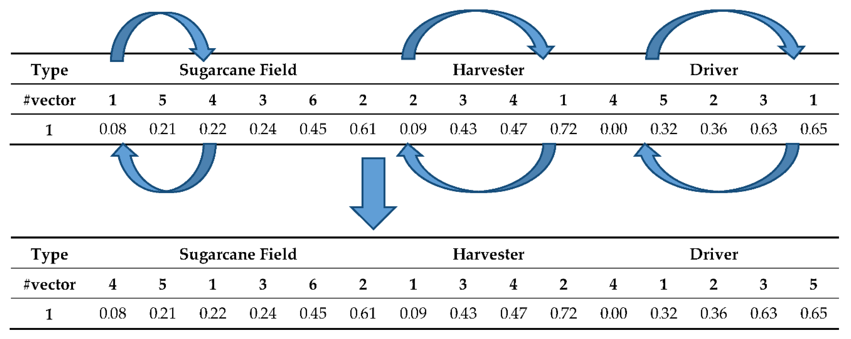
The swap algorithm will be applied to all three sets of vectors when we carry out the local search. For example, we have a current vector, as shown in Figure 3. If the swap is performed on sugarcane field positions 1 and 3, harvester sets 1 and 4, and drivers 2 and 5. Then new vectors for each item are obtained.

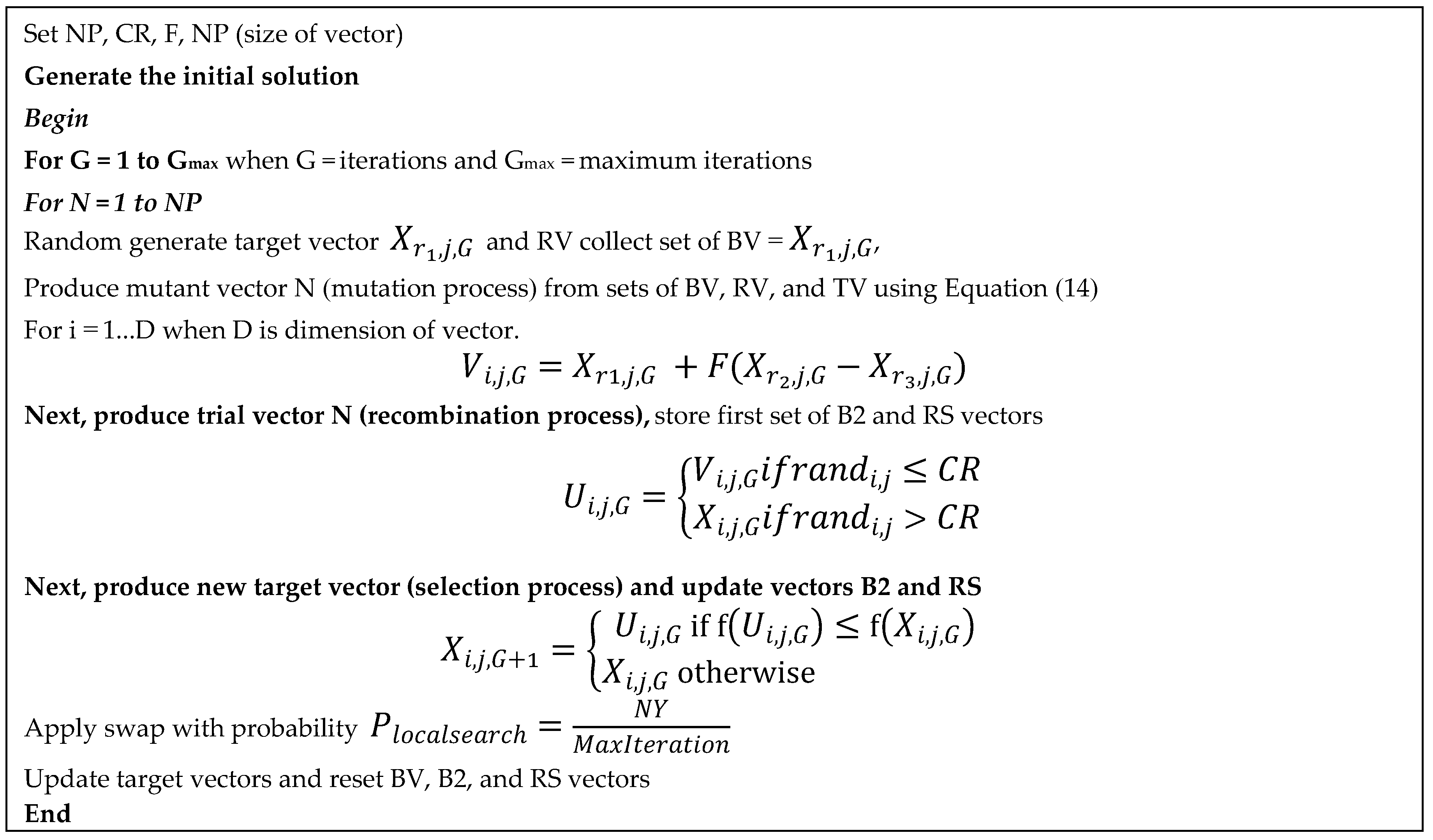
From Figure 3, we can see that only the field number is rearranged and the value in every position remains the same. Therefore, after applying the decoding method, the solution changes. The swap will be applied to every entity or position of a vector. A decoding method is always applied to a pair of vectors that have been swapped. The same process is applied for BV, B2, and RS vectors. In total, 3 × NP vectors are searched, and the best NP vector is used as the new target vector in iteration G + 1. The current BV, B2, and RS are newly initialized whenever the local search is performed. The modified DE is concluded in Figure 4.

4. Computational Framework and Results

The proposed heuristics was coded in Dev C++ using a PC with Intel Core i3 CPU 3.70 GHz Ram DDR4 8 GB. The parameters of the proposed heuristics were set to be the same as in the literature (Pitakaso and Sethanan (2016)), which is Cr = 0.8, F = 1.5, and NP = 10. 9. Randomly generated data were formed and tested for the effectiveness of the algorithm by comparing with the best solution and the lower bound obtained from Lingo v.11. The case study was executed as 15 cases. The details of the test instances are given in

Table 10. Characteristics of test instances and case study.

#Instances	#Fields	#Harvesters	#Drivers	#Instances	#Fields	#Harvesters	#Drivers
1	6	4	5	6	20	21	22
2	6	5	5	7	25	27	23
3	15	13	12	8	30	23	26
4	15	16	18	9	35	28	35
5	20	19	23	Case study	73	62	69

.

The number of fields ranges from 6 to 73 to represent small to large problems. The numbers of harvester sets and drivers were selected to represent all cases. For example, the number of harvester sets could be higher or lower than the number of fields, and the number of drivers could be higher or lower than the numbers of fields and harvester sets. The number of harvester sets ranges from 4 to 62, and the number of drivers ranges from 5 to 69.

Table 11. Values of parameters.

Parameter	Min Value	Max Value	Parameter	Min Value	Max Value
Ak	20	120	Ri	0.6	1.4
bk	0.6	1.5	Pi	0.7	1.5
Ej	80	210	Tj	6	14
Uj	1.0	1.7

shows the values of parameters used in this proposed problem. In this case study, the minimum and maximum number of each parameter is selected from the real maximum and minimum value.

The proposed problem is solved by using three DE algorithms, DE-1, DE-2, and DE-3, characteristics, which are shown in

Table 12. Definitions of Lingo v.11 solutions and the proposed algorithm.

Algorithm	Min Value
L1	Optimal solution obtained from Lingo
LU	Upper bound of Lingo given within 96 h
LB	Best solution given by Lingo within 96 h
DE	Original DE
MDE-1	Modified DE without a local search
MDE-2	Modified DE with a local search
MDE-3	MDE-2 without using RV
MDE-4	MDE-2 without using BV

.

Table 12 gives details and definitions of the simulation test. Lingo v.11′s limited maximum time is 96 h or 5760 min, and the DE and MDE’s stopping criterion is the number of iterations, which was set at 1000. The solution of the test instances is shown in

Table 13. Profit generated from different methods.

#Instances	Type	L1	LU	LB	DE	MDE-1	MDE-2	MDE-3	MDE-4
1	Profit	102,954	102,954	102,954	102,954	102,954	102,954	102,954	102,954
	Comp	1.45	1.45	1.45	1.1	1.1	1.3	1.2	1.2
2	Profit	176,097	176,097	176,097	176,097	176,097	176,097	176,097	176,097
	Comp	10.31	10.31	10.31	3.5	3.9	4.12	4.01	4.03
3	Profit	N/A	359,128	332,591	341,258	347,217	351,831	346,136	346,283
	Comp	5760	5760	5760	5.88	5.98	6.43	6.32	6.36
4	Profit	N/A	479,129	438,219	441,258	445,981	467,193	451,821	450,562
	Comp	5760	5760	5760	4.23	5.12	5.89	5.43	5.41
5	Profit	N/A	589,182	559,129	560,821	568,127	579,812	568,213	568,129
	Comp	5760	5760	5760	13.43	15.43	16.23	15.89	15.81
6	Profit	N/A	678,684	632,152	642,518	647,561	667,246	653,412	652,954
	Comp	5760	5760	5760	21.56	22.15	24.32	23.59	24.12
7	Profit	N/A	741,282	711,242	722,568	724,125	731,562	728,159	727,151
	Comp	5760	5760	5760	23.34	25.45	26.75	25.61	25.89
8	Profit	N/A	812,875	789,822	792,831	799,284	806,542	800,212	800,512
	Comp	5760	5760	5760	30.12	33.54	35.42	34.18	34.03
9	Profit	N/A	1,192,123	1,042,318	1,082,675	1,091,786	1,130,941	1,100,878	1,100,765
	Comp	5760	5760	5760	45.54	48.43	50.23	49.54	50.14
Case study	Profit	N/A	2,812,411	2,524,612	2,618,124	2,627,619	2,684,982	2,635,124	2,649,218
	Comp	5760	5760	5760	60.43	65.89	70.73	69.45	68.76

. The best solution generated from each method is recorded. In this case, Lingo v.11 can find the optimal solution before 5760 min of computational time is recorded. For the proposed heuristics, the best solution generated during 1000 iterations is recorded, and the computational time of 1000 iterations is shown in Table 13.

Table 13 shows the computational results of 10 test instances. To have a better conclusion, the paired t-test was used to check the differences of each method. The results of the statistical tests are shown in

Table 14. Statistical test results (paired t-test).

	LB	DE	MDE-1	MDE-2	MDE-3	MDE-4
LU	> 0.026	> 0.066	> 0.025	> 0.043	> 0.029	> 0.025
LB	-	< 0.048	< 0.027	< 0.017	< 0.022	< 0.028
DE	-	-	< 0.001	< 0.005	< 0.0001	< 0.006
MDE-1	-	-	-	< 0.009	< 0.011	< 0.036
MDE-2	-	-	-	-	> 0.011	> 0.005
MDE-3	-	-	-	-	-	= 0.221

.

From Table 14, we can see that all proposed heuristics give better solutions than the best solution obtained from Lingo v.11 (LB). We can conclude from Table 14 that the order of algorithms from the best to worst performing methods is MDE-2, MDE-3, MDE-4, MDE-1, and DE. There is no evidence to show that MDE-3 and MDE-4 are different from one another, but they are different from all the other heuristics.

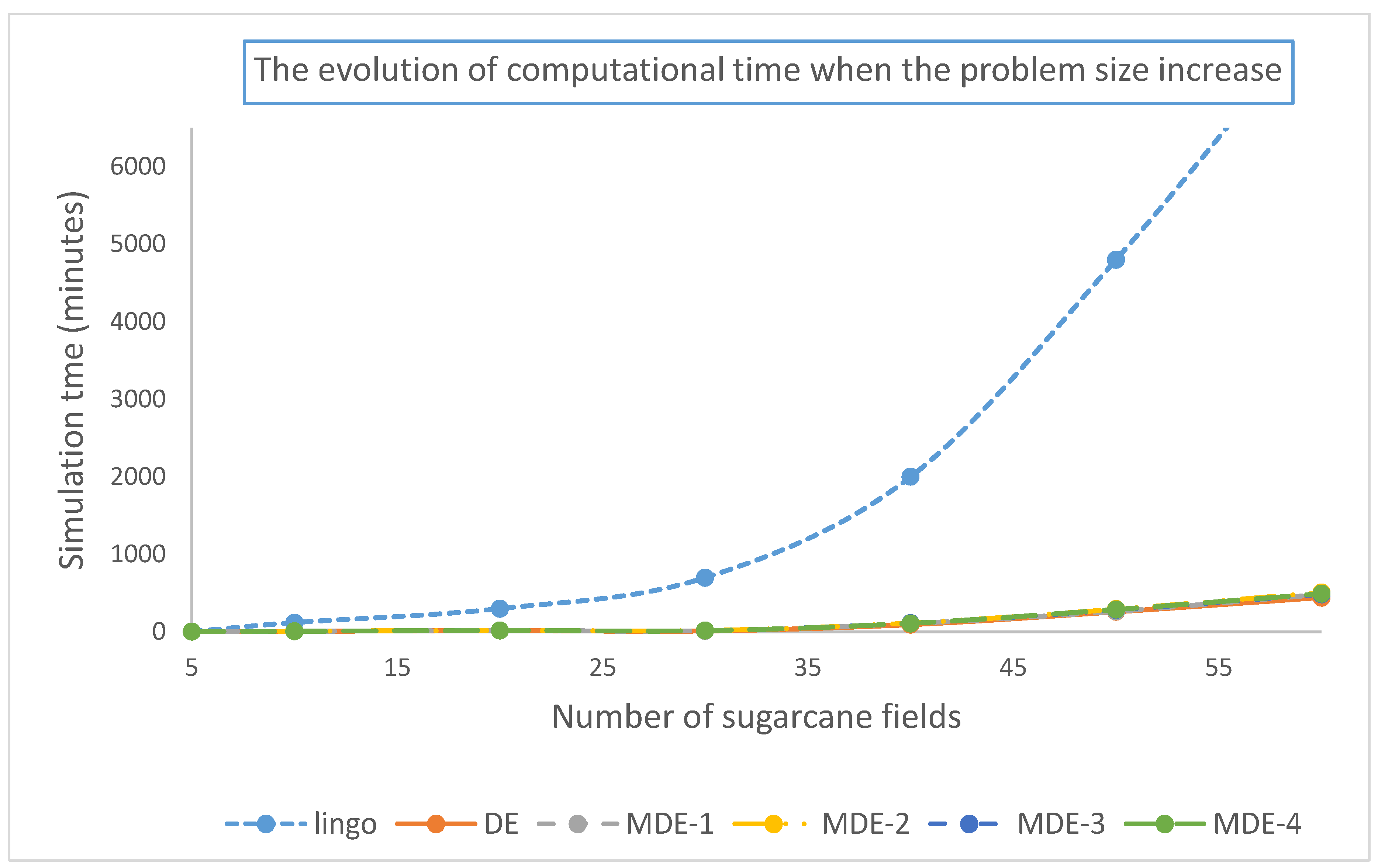
At this point, we discovered why each of the proposed heuristics is different. We use the computational time to plot and visualize the evolution of using computational time of each proposed heuristic using Lingo v.11, and the results are shown in Figure 5.

From Figure 5, we can see that Lingo v.11 computational time exponentially increases as the size of the problem increases, while, for DE and MDE, the computational time gradually increases, but the growth is relatively low.

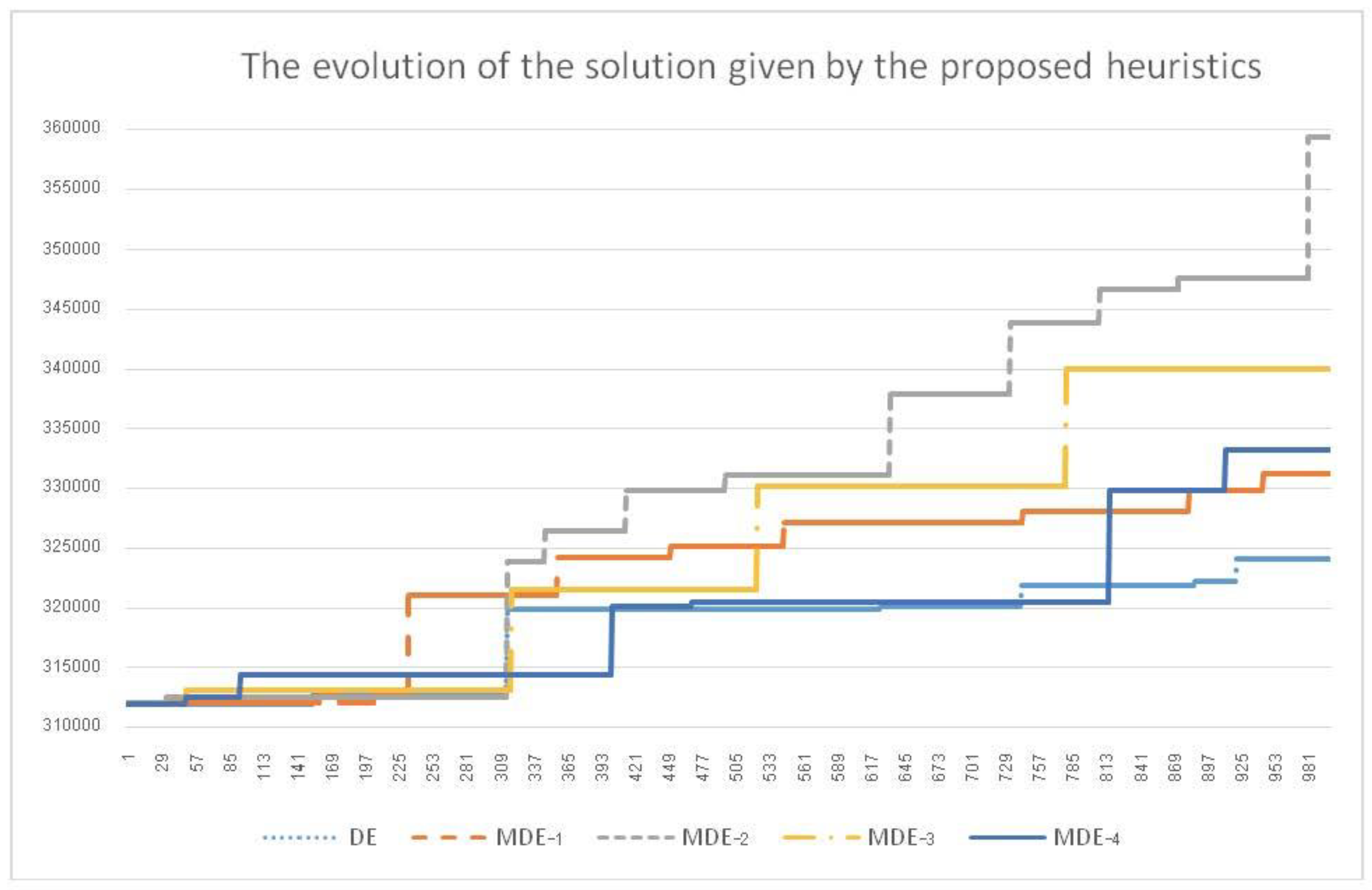
Figure 6 shows the evolution of the proposed heuristics in finding a solution when the iteration is longer.

From Figure 6, we can see that the general DE is the worst heuristic to find a satisfactory solution. This because the DE does not have the guide from the best solution. The current target vector has a good algorithm search for the good solution, but it did not improve the solution quality. The second worst solution is MDE-1, which is the DE that uses the guide from the good solution (BV-vector), but it does not have a local search. We can see from the behavior of this algorithm that it can always find better solutions, but, when finding a new solution, the solution quality stays the same and does not change so much. This means that the algorithm is guided by the good solution (BV-vector) and also escapes from the local optimal (RV-vector). However, the solution does not change much each time it finds a better solution. MDE-2, MDE-3, and MDE-4 perform similarly to one another, since they can often find new solutions. However, the only difference is that MDE-4 seems to change less often when finding the new best solution due to the fact that it does not use the guide from the best vector (BV). It introduces only the random vector to the current vector, and, therefore, the guide to a good area, which allows the local search to perform better. This is lost from the algorithm. MDE-3 can find a good solution in a very short amount of time, and when it finds a good solution, it sticks to that area long before it can find a new best solution. The reason for this is that it sticks onto the local optimal since it is the fastest converse heuristic, which comes from the guide of the best vector (BV) to a good area but does not introduce the random vector (RV) to escape from the local optimal. Therefore, it loses its diversification. Lastly, MDE-2 is the compensation of MDE-3 and MDE-4 and has both diversification and intensification behavior. Hence, MDE-2 outperforms all other proposed heuristics in finding a good solution.

Fuel consumption is one of the main expenses for harvesting. According to the results above, three strategies are presented here to reduce the total cost. (1) The change harvesters that are already in use for more than five years, which can reduce the energy consumption rate affected by the engine (U_j = 1.0 for all J), (2) train all drivers so they have an experience level of at least 1.0, and (3) change engines and train drivers (combination of 1 and 2). Strategy 1 requires an investment of 15,000,000 baht. Strategy 2 requires an investment of 5,000,000 baht, and strategy 3 requires 20,000,000 baht. We used MDE-2 to execute these three strategies and calculate break-even points (days), as shown in

Table 15. Break-even (days) for three proposed strategies.

	Current Cost	Change Engines	Train Drivers	Change Engines + Train Drivers
Case study	2,684,982	2,646,689	2,641,245	2,621,451
Investment	-	15,000,000	5,000,000	20,000,000
Diff–Profit	-	38,293	43,737	63,531
Break-even(days)	-	391.716502	114.319684	314.806945

.

From Table 15, the most beneficial strategy for the company is to train drivers because it only needs 114,319 days to return all investment. Nonetheless, this strategy deals with human beings, which involves more factors that have to be taken into account, such as emotions and intelligence of the drivers (not everyone can be trained). Changing engines needs 391,716 days to return all investments, which is not long. After that, in up to five years, it will generate profit for the company.

5. Conclusions and Outlook

This paper presents a methodology to solve a special case of the generalized assignment problem (S-GAP). The problem is composed of assigning drivers to harvesters and then harvesters to sugarcane fields in order to maximize daily profit. The drivers have different levels of experience, which means they have a different capability to harvest sugarcane and different levels of daily wages. The harvesters have been used for different periods of time, which affects their fuel consumption rate. Harvesters have different sizes and different capacities to harvest sugarcane. Assigning workers to harvesters can change the fuel usage and harvest rate of the harvesters.

We developed a mathematical model and solved the problem optimally by commercial optimization software. It can only solve a very small problem (see Table 14). Five heuristics have been presented to solve the problem more effectively for a larger size of test instances. One of these five methods is the differential evolution algorithm and the other four are modified differential evolution algorithms MDE-1, MDE-2, MDE-3, and MDE-4. MDE-1 uses Equations (12)–(14) to generate the mutation vector, which is the product of BV-vectors, RV-vectors, and TV-vectors, instead of using only TV-vector, like the original DE. The probability of using the best vector (BV), the random vector (RV), and the target vector (TV) in the mutation process employs the idea of the attractiveness of each group of vectors. MDE-2 is MDE-1 with a swap algorithm added to the mechanism. The swap will be the probability to commence. The probability of using swap increases when the number of iterations that the new best solution uses rises.

The computational result shows that when Lingo v.11 finds the optimal solution, all proposed heuristics can also find the optimal solution, but they use less computational time. When the size of the problem increases, the capability of Lingo finding the solution reduces. The computational time of Lingo v.11 exponentially increases, while that of the other proposed heuristics slightly increases. Comparing all proposed heuristics, MDE-2 is significantly better than all the others due to the fact that it has both diversification (the use of RV-vector) and intensification (the use of BV-vector and local search).

The local search, which is applied to three sets of vectors, best vector (BV), second best vector (B2), and randomly selected vector (RS), is helpful. It increases the solution quality of the proposed heuristics. MDE-1 is the only MDE that has no local search, and it generates a worse solution than the other methods.

Moreover, we tried to increase daily profit by presenting three management strategies: (1) change all harvesters that are more than five years old, (2) train drivers to reach the maximum capacity, and (3) use a combination of 1 and 2. Each strategy requires a different investment. The daily profit was simulated from MDE-2. The increased profit from the original MDE-2 was compared with the investment of each strategy. The computational result shows that strategy 2 is the best due to the fact that it has a lower break-even point (it requires the smallest number of days to return the investment), but it has a weak point since drivers will not always have full working capacity. The drivers may quit the company if they gain too much of a driving skill. Strategy 1 is within the acceptable break-even time, which may return all investments within 392 days.

From the computational result, we can conclude that metaheuristics like DE can successfully solve the proposed problem. The other metaheuristics, which has an excellent search mechanism such as the polar bear optimization [36], the Dragonfly algorithm [37], and the whale optimization algorithm [38], should successfully solve the proposed problem. The proposed algorithm can be more interesting if it can find the maximum profit for the farmers and keep the maximum income for the drivers so that they are willing to follow the constructed plan. This will turn the proposed problem from GAP to muti-objective GAP, which is also applicable to solve by DE and other heuristics addressed above.

The article presents very successful algorithms to solve the problem. The sugarcane business is one out of the most important business in Thailand. Each year, more than 10,000 million Baht circulate in this business. The algorithm that we propose is not only used to solve the specific problem, but also can solve the related problem. Enhancing the capability of the algorithm, a good software design is needed. When the software finished the related business, it can customize the software and share the license or patent of the developed software. Therefore, it is not limited only in the sugarcane business. Therefore, the open innovation concept has been applied to the sugarcane and the related business sector. The goal of open innovative is to be successful in business even if it has rapid changes in the business environment by buying, sharing, researching, developing, and more. An example of open innovation research studies can be revealed in Yun et al. [39] and Yun et al. [40].