
A Hybrid Grey Wolf Optimization Algorithm Using Robust Learning Mechanism for Large Scale Economic Load Dispatch with Vale-Point Effect


Abstract
1. Introduction
2. Problem Formulation
2.1. Objective Function
2.2. Equality and Inequality Constraints
- (a)
- Active power balance constraintThe total generated power output should be the same as the sum of the total power demand and the total system loss . This is represented as follows:
- (b)
- The limitations of the generatorThe power output of each generating unit should be limited to between its minimum and maximum power outputs, as shown in the inequality constraint in (6):where and are the minimum and maximum real power output of the generating unit i.
3. GWO Algorithm
3.1. Social Hierarchy
3.2. Encircling Prey
3.3. Hunting
4. Robust Learning-Based GWO Algorithm (RLGWO)
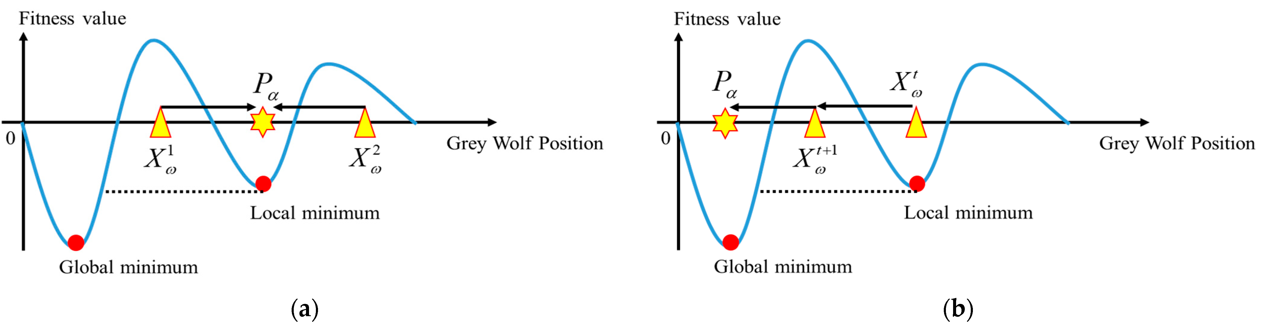
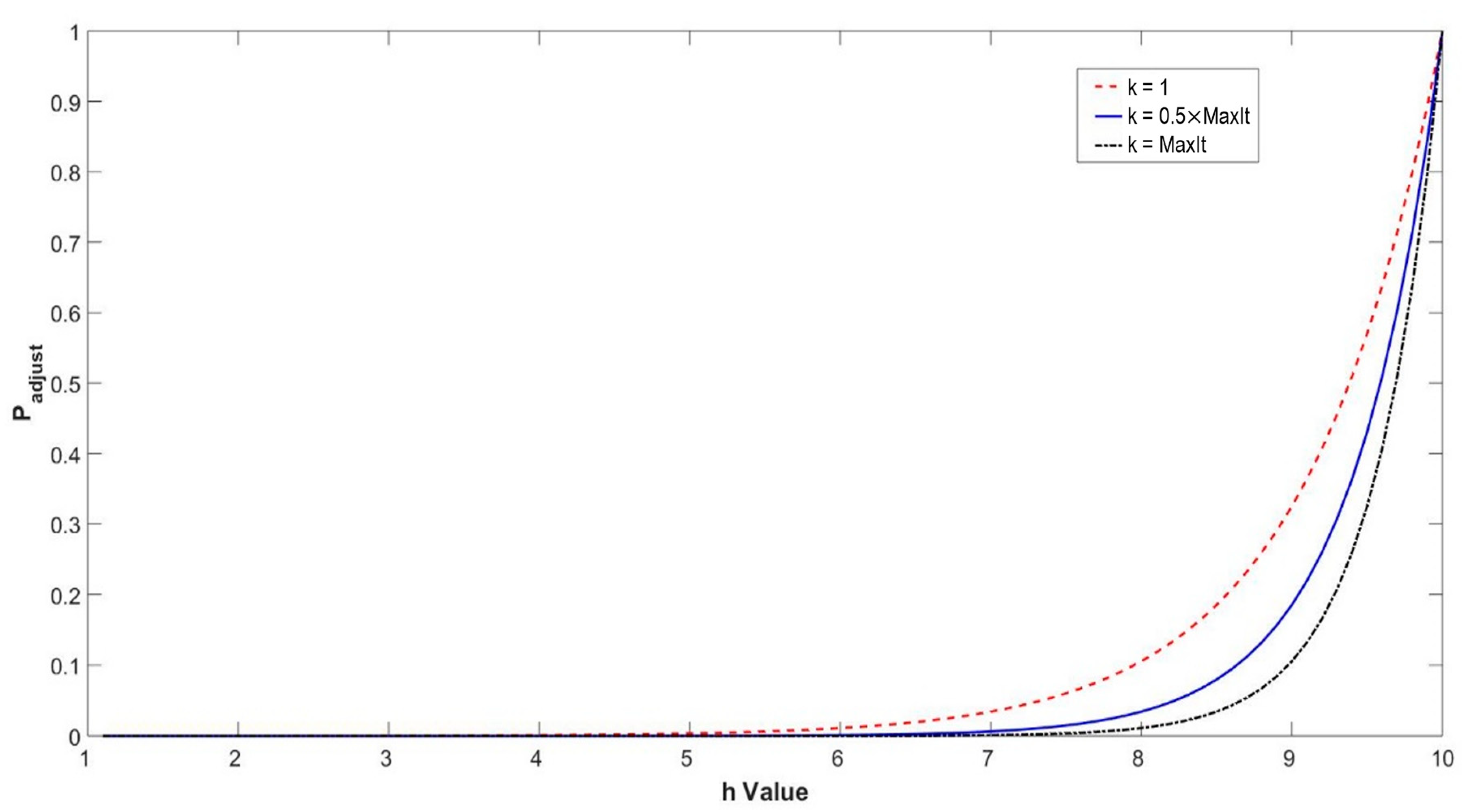
4.1. Robust Tolerance-Based Adjust Searching Direction Mechanism (RTASDM)
| Algorithm 1. Robust tolerance-based adjust searching direction mechanism |
| 1: At iteration kth; |
| then |
| 5: end if |
| 6: generate a random number in the range of [0,1]; |
| then |
| 8: Finding another candidate solution to replace alpha (beta or gamma) |
| 9: end if |
4.2. Opposition-Based Learning for Candidate Generation Strategy
| Algorithm 2. Opposition-based learning for candidate generation strategy |
| 1: At iteration kth; |
| between [0,1]; |
| 4: Keep alpha, beta, and gamma as the leader; |
| 5: else |
| then |
| ; |
| 8: else |
| between [0,1]; |
| ; |
| 12: else |
| ; |
4.3. RLGWO Algorithm for Economic Load Dispatch
5. Simulation Results and Discussion
5.1. Test Systems and Results
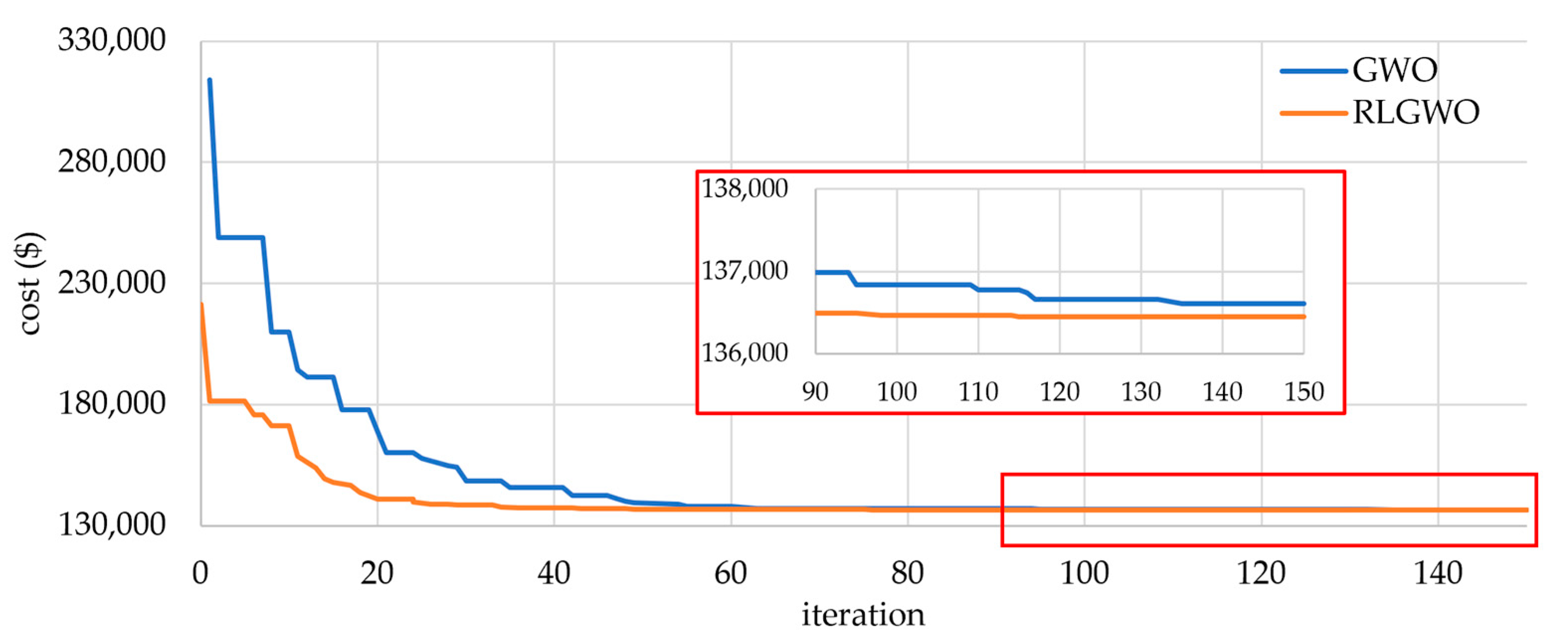
5.1.1. Test System 1
5.1.2. Test System 2
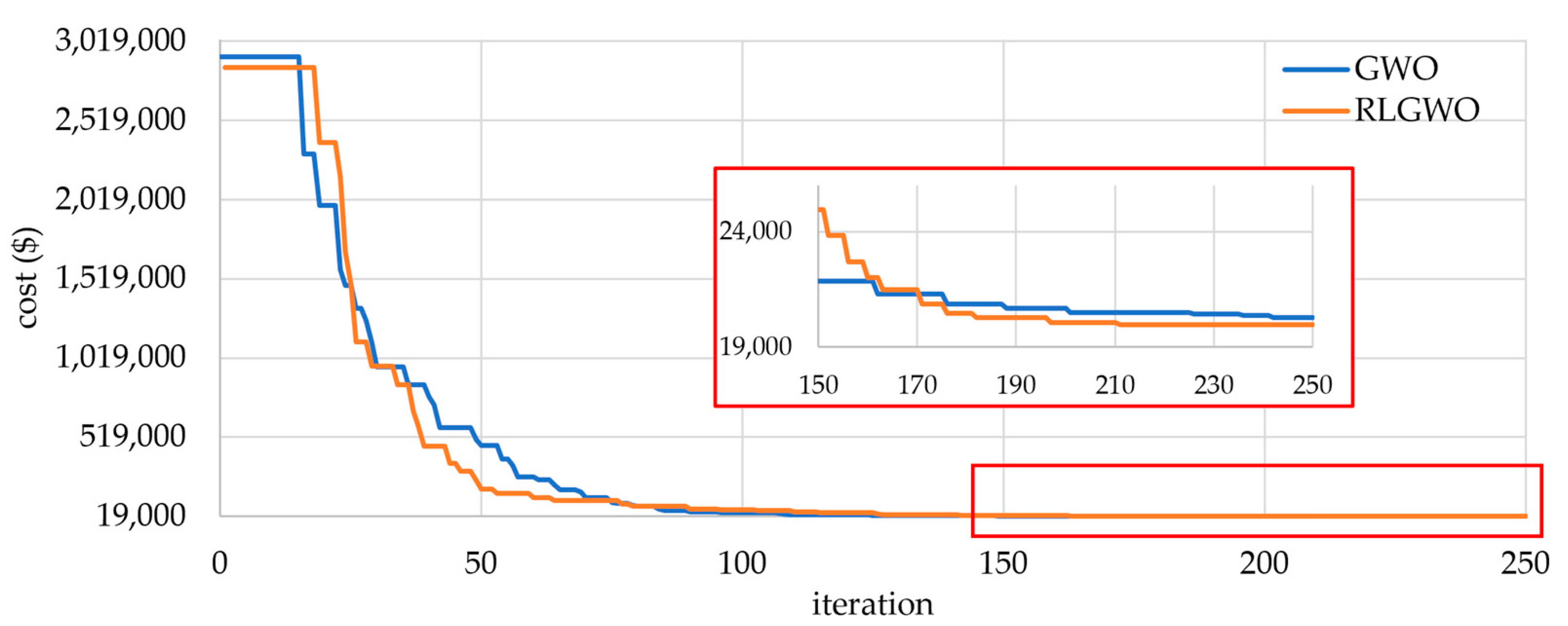
5.1.3. Test System 3
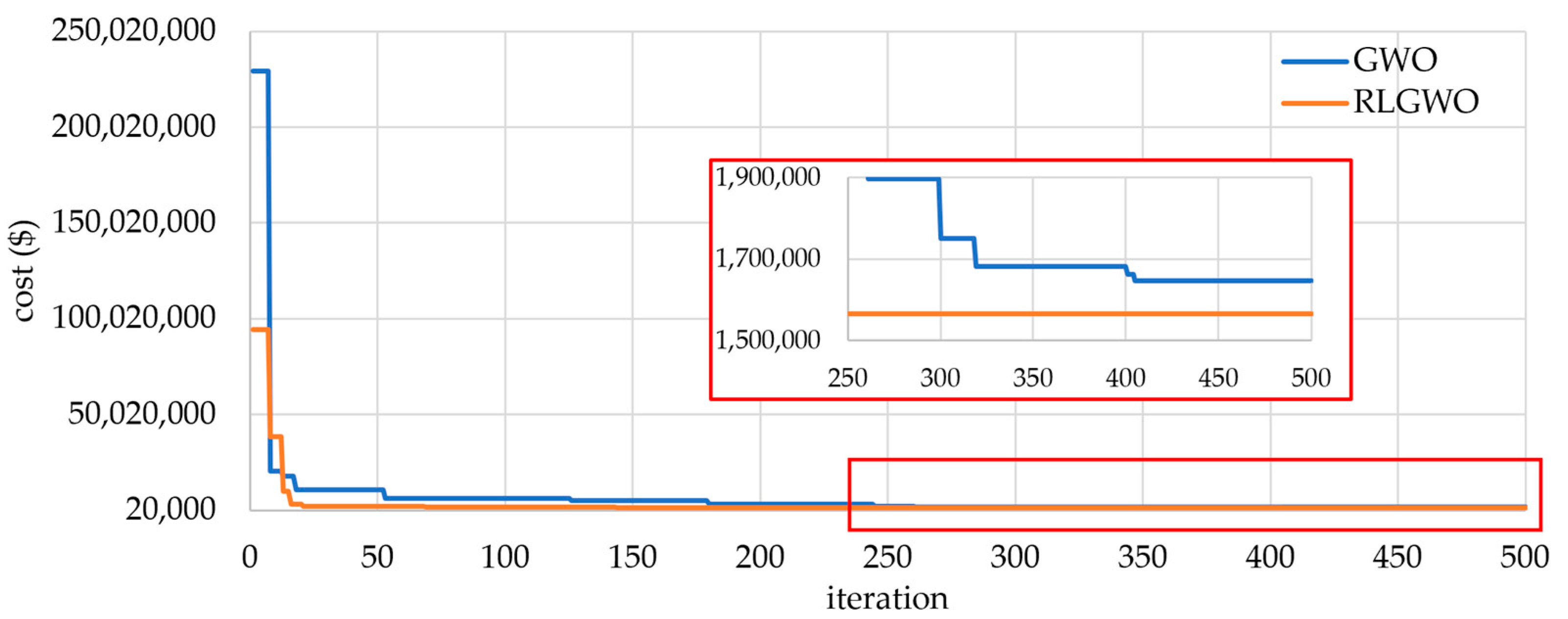
5.1.4. Test System 4
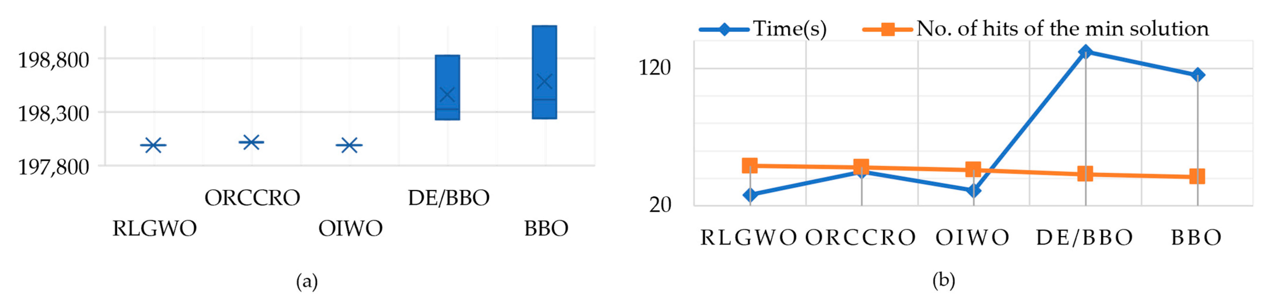
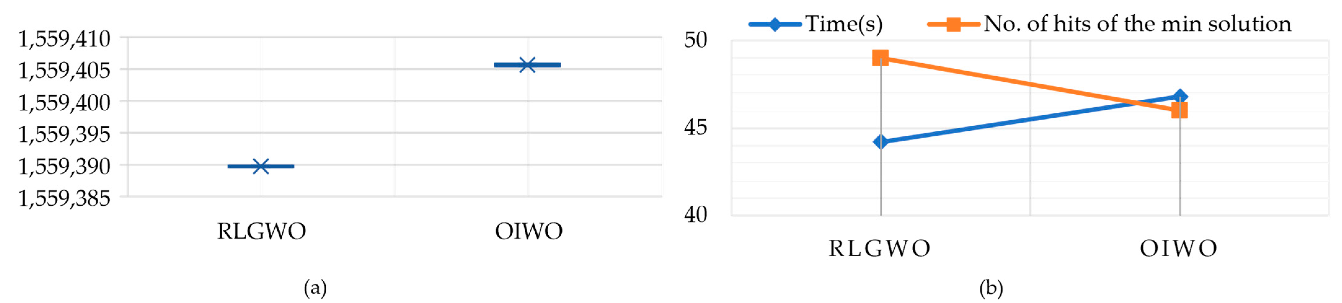
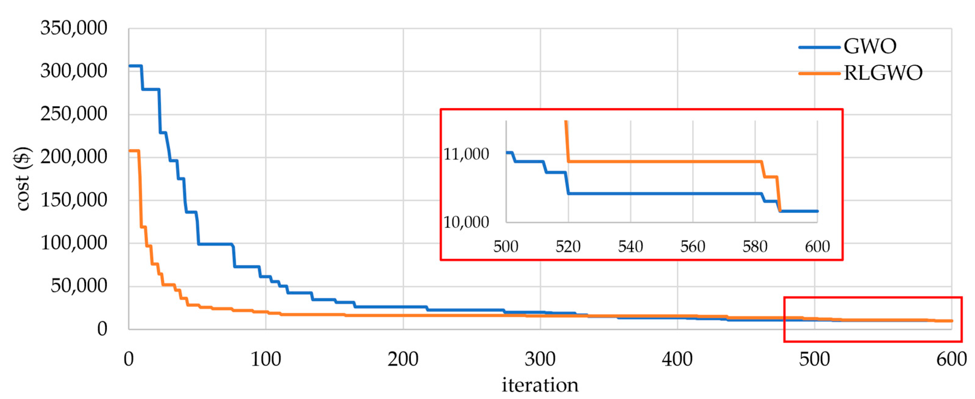
5.1.5. Test System 5
5.2. Comparative Study
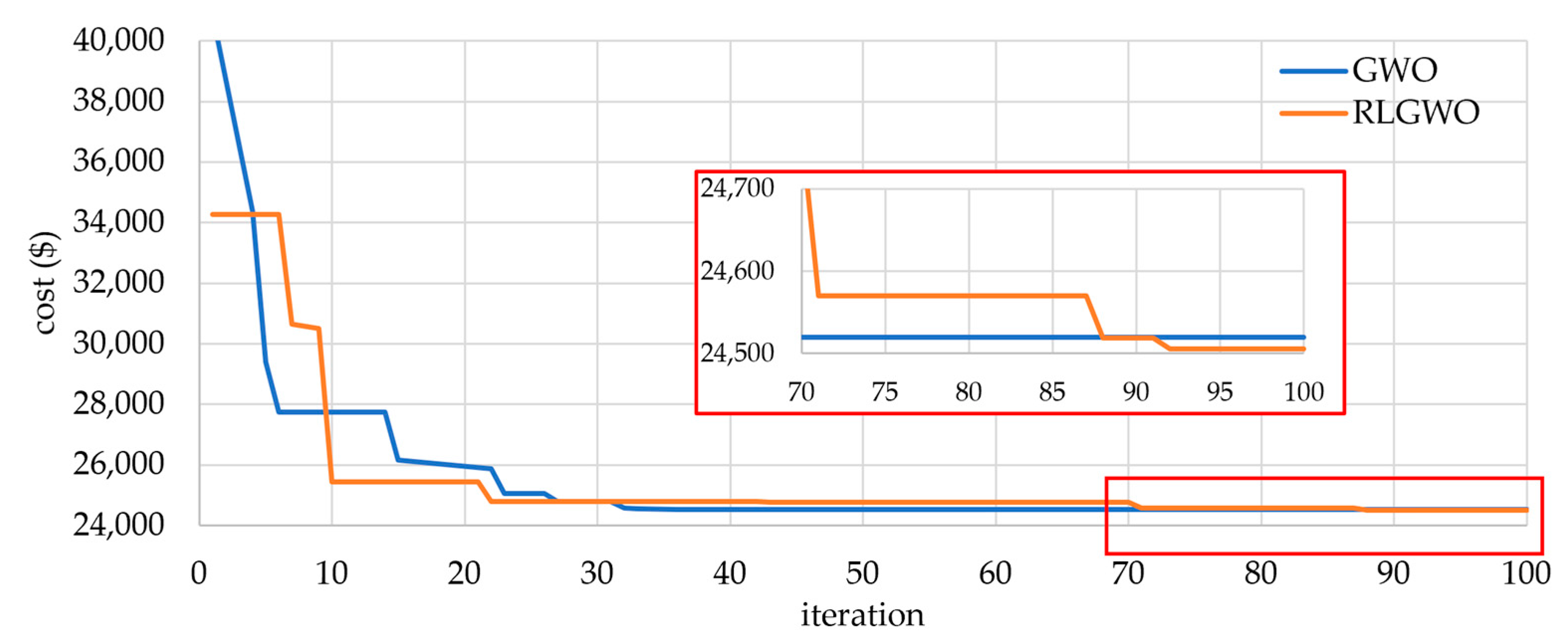
5.2.1. Solution Quality
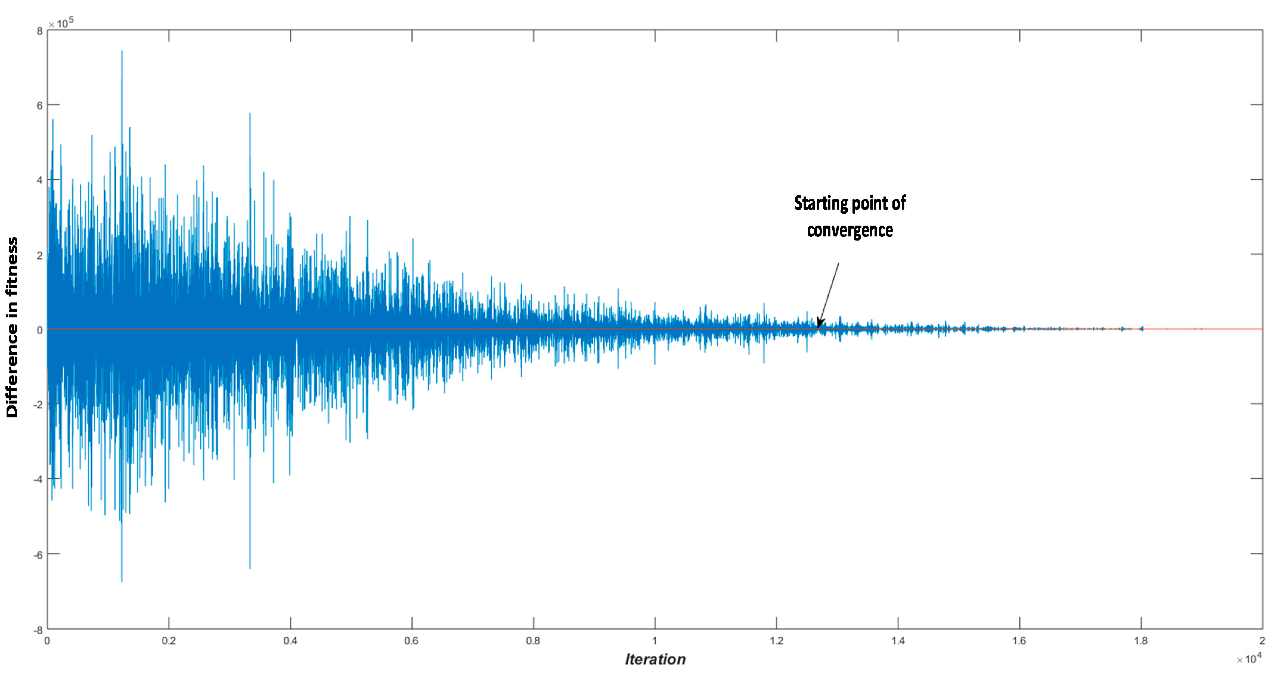
5.2.2. Computational Efficiency and Robustness
6. Conclusions and Future Work
Author Contributions
Funding
Institutional Review Board Statement
Informed Consent Statement
Data Availability Statement
Acknowledgments
Conflicts of Interest
References
- Chakraborty, S.; Senjyu, T.; Yona, A.; Saber, A.; Funabashi, T. Solving economic load dispatch problem with valve-point effects using a hybrid quantum mechanics inspired particle swarm optimisation. IET Gener. Transm. Distrib. 2011, 5, 1042–1052. [Google Scholar] [CrossRef]
- Wood, A.J.; Wollenberg, B.F.; Sheblé, G.B. Power Generation, Operation, and Control, 3rd ed.; Wiley-Interscience: Hoboken, NJ, USA, 2014. [Google Scholar]
- Lee, K.Y.; Park, Y.M.; Ortiz, J.L. Fuel-cost minimisation for both real-and reactive-power dispatches. IEE Proc. C (Gener. Transm. Distrib.) 1984, 131, 85–93. [Google Scholar] [CrossRef]
- Sasson, A.M. Nonlinear Programming Solutions for Load-Flow, Minimum-Loss, and Economic Dispatching Problems. IEEE Trans. Power Appar. Syst. 1969, PAS-88, 399–409. [Google Scholar] [CrossRef]
- Liang, Z.-X.; Glover, J.D. A zoom feature for a dynamic programming solution to economic dispatch including transmission losses. IEEE Trans. Power Syst. 1992, 7, 544–550. [Google Scholar] [CrossRef]
- Wong, K.; Fung, C. Simulated annealing based economic dispatch algorithm. IEE Proc. C Gener. Transm. Distrib. 1993, 140, 509–515. [Google Scholar] [CrossRef]
- Chen, P.-H.; Chang, H.-C. Large-scale economic dispatch by genetic algorithm. IEEE Trans. Power Syst. 1995, 10, 1919–1926. [Google Scholar] [CrossRef]
- Lin, W.-M.; Cheng, F.-S.; Tsay, M.-T. An improved tabu search for economic dispatch with multiple minima. IEEE Trans. Power Syst. 2002, 17, 108–112. [Google Scholar] [CrossRef]
- Ruey-Hsum, L. A neural-based redispatch approach to dynamic generation allocation. IEEE Trans. Power Syst. 1999, 14, 1388–1393. [Google Scholar] [CrossRef]
- Yalcinoz, T.; Short, M.J. Neural networks approach for solving economic dispatch problem with transmission capacity constraints. IEEE Trans. Power Syst. 1998, 13, 307–313. [Google Scholar] [CrossRef]
- Gaing, Z.-L. Particle swarm optimization to solving the economic dispatch considering the generator constraints. IEEE Trans. Power Syst. 2003, 18, 1187–1195. [Google Scholar] [CrossRef]
- Park, J.B.; Shin, J.R.; Lee, K.Y. Closure to discussion of “An improved particle swarm optimization for nonconvex economic dispatch prob-lems”. IEEE Trans. Power Syst. 2010, 25, 2010–2011. [Google Scholar] [CrossRef]
- Bhattacharya, A.; Chattopadhyay, P.K. Biogeography-Based Optimization for Different Economic Load Dispatch Problems. IEEE Trans. Power Syst. 2009, 25, 1064–1077. [Google Scholar] [CrossRef]
- Chiang, C.-L. Improved genetic algorithm for power economic dispatch of units with valve-point effects and multiple fuels. IEEE Trans. Power Syst. 2005, 20, 1690–1699. [Google Scholar] [CrossRef]
- Djokić, S.Ž.; Milanović, J.V.; Rowland, S.M. Advanced voltage sag characterisation II: Point on wave. IET Gener. Trans-Mission. Distrib. 2007, 1, 146–154. [Google Scholar] [CrossRef]
- Noman, N.; Iba, H. Differential evolution for economic load dispatch problems. Electr. Power Syst. Res. 2008, 78, 1322–1331. [Google Scholar] [CrossRef]
- Hou, Y.H.; Wu, W.; Xiong, X. Economic dispatch of power systems based on generalized ant colony optimization method. Zhongguo Dianji Gongcheng Xuebao/Proc. Chin. Soc. Electr. Eng. 2003, 23, 59. [Google Scholar]
- Coelho, L.D.S.; Mariani, V.C. Correction to “Combining of Chaotic Differential Evolution and Quadratic Programming for Economic Dispatch Optimization with Valve-Point Effect”. IEEE Trans. Power Syst. 2006, 21, 1465. [Google Scholar] [CrossRef]
- Vitthaladevuni, P.K.; Alouini, M.S. Discussion of “Economic Load Dispatch-A Comparative Study on Heuristic Optimi-zation Techniques With an Improved Coordinated Aggregation-Based PSO”. IEEE Trans. Broadcast. 2003, 49, 408. [Google Scholar] [CrossRef]
- Meng, K.; Wang, H.G.; Dong, Z.; Wong, K.P. Quantum-Inspired Particle Swarm Optimization for Valve-Point Economic Load Dispatch. IEEE Trans. Power Syst. 2009, 25, 215–222. [Google Scholar] [CrossRef]
- Roy, P.; Roy, P.; Chakrabarti, A. Modified shuffled frog leaping algorithm with genetic algorithm crossover for solving economic load dispatch problem with valve-point effect. Appl. Soft Comput. 2013, 13, 4244–4252. [Google Scholar] [CrossRef]
- Bhattacharya, A.; Chattopadhyay, P.K. Hybrid Differential Evolution With Biogeography-Based Optimization for Solution of Economic Load Dispatch. IEEE Trans. Power Syst. 2010, 25, 1955–1964. [Google Scholar] [CrossRef]
- Dai, C.; Hu, Z.; Su, Q. An adaptive hybrid backtracking search optimization algorithm for dynamic economic dispatch with valve-point effects. Energy 2021, 239, 122461. [Google Scholar] [CrossRef]
- Barisal, A.K.; Prusty, R.C. Large scale economic dispatch of power systems using oppositional invasive weed optimization. Appl. Soft Comput. 2015, 29, 122–137. [Google Scholar] [CrossRef]
- Tizhoosh, H.R. Opposition-Based Learning: A New Scheme for Machine Intelligence. In Proceedings of the International Conference on Com-putational Intelligence for Modelling, Control and Automation and International Conference on Intelligent Agents, Web Technologies and Internet Commerce (CIMCA-IAWTIC’06), Vienna, Austria, 28–30 November 2005. [Google Scholar]
- Mirjalili, S.; Mirjalili, S.M.; Lewis, A. Grey Wolf Optimizer. Adv. Eng. Softw. 2014, 69, 46–61. [Google Scholar] [CrossRef]
- El-Fergany, A.A.; Hasanien, H.H. Single and Multi-objective Optimal Power Flow Using Grey Wolf Optimizer and Dif-ferential Evolution Algorithms. Electr. Power Compon. Syst. 2015, 43, 1548–1559. [Google Scholar] [CrossRef]
- Shakarami, M.R.; Faraji, I. Design of SSSC-based Stabilizer to Damp Inter-Area Oscillations Using Gray Wolf Optimization Algorithm. 2015. Available online: https://sid.ir/paper/907750/en (accessed on 13 February 2023).
- Bhattacharjee, K.; Bhattacharya, A.; Dey, S.H.N. Oppositional Real Coded Chemical Reaction Optimization for different economic dispatch problems. Int. J. Electr. Power Energy Syst. 2014, 55, 378–391. [Google Scholar] [CrossRef]
- Sinha, N.; Chakrabarti, R.; Chattopadhyay, P.K. Evolutionary programming techniques for economic load dispatch. IEEE Trans. Evol. Comput. 2003, 7, 83–94. [Google Scholar] [CrossRef]
- Muro, C.; Escobedo, R.; Spector, L.; Coppinger, R. Wolf-pack (Canis lupus) hunting strategies emerge from simple rules in computational simulations. Behav. Process. 2011, 88, 192–197. [Google Scholar] [CrossRef]
- Long, W.; Jiao, J.; Liang, X.; Tang, M. An exploration-enhanced grey wolf optimizer to solve high-dimensional numerical optimization. Eng. Appl. Artif. Intell. 2018, 68, 63–80. [Google Scholar] [CrossRef]
- Gaidhane, P.J.; Nigam, M.J. A hybrid grey wolf optimizer and artificial bee colony algorithm for enhancing the performance of complex systems. J. Comput. Sci. 2018, 27, 284–302. [Google Scholar] [CrossRef]
- Wang, F.; Zhang, H.; Li, K.; Lin, Z.; Yang, J.; Shen, X.-L. A hybrid particle swarm optimization algorithm using adaptive learning strategy. Inf. Sci. 2018, 436–437, 162–177. [Google Scholar] [CrossRef]
- Shaw, B.; Mukherjee, V.; Ghoshal, S. A novel opposition-based gravitational search algorithm for combined economic and emission dispatch problems of power systems. Int. J. Electr. Power Energy Syst. 2012, 35, 21–33. [Google Scholar] [CrossRef]
- Chatterjee, A.; Ghoshal, S.; Mukherjee, V. Solution of combined economic and emission dispatch problems of power systems by an opposition-based harmony search algorithm. Int. J. Electr. Power Energy Syst. 2012, 39, 9–20. [Google Scholar] [CrossRef]
- Mandal, B.; Roy, P.K. Optimal reactive power dispatch using quasi-oppositional teaching learning based optimization. Int. J. Electr. Power Energy Syst. 2013, 53, 123–134. [Google Scholar] [CrossRef]
- Ergezer, M.; Simon, D. Oppositional biogeography-based optimization for combinatorial problems. In Proceedings of the 2011 IEEE Congress of Evolutionary Computation (CEC), New Orleans, LA, USA, 5–8 June 2011. [Google Scholar]
- Reddy, A.S.; Vaisakh, K. Shuffled differential evolution for large scale economic dispatch. Electr. Power Syst. Res. 2013, 96, 237–245. [Google Scholar] [CrossRef]
- Ciornei, I.; Kyriakides, E. A GA-API Solution for the Economic Dispatch of Generation in Power System Operation. IEEE Trans. Power Syst. 2011, 27, 233–242. [Google Scholar] [CrossRef]
- Orero, S.O.; Irving, M.R. Large scale unit commitment using a hybrid genetic algorithm. Int. J. Electr. Power Energy Syst. 1997, 19, 45–55. [Google Scholar] [CrossRef]


| Unit Number | Methods | |||
|---|---|---|---|---|
| RLGWO | SDE | OIWO | ORCCRO | |
| 1 | 628.3112 | 628.32 | 628.3185 | 628.32 |
| 2 | 299.1788 | 299.2 | 299.1989 | 299.2 |
| 3 | 299.1798 | 299.2 | 299.1991 | 299.2 |
| 4 | 159.7297 | 159.73 | 159.7331 | 159.73 |
| 5 | 159.7297 | 159.73 | 159.7331 | 159.73 |
| 6 | 159.7297 | 159.73 | 159.7331 | 159.73 |
| 7 | 159.7284 | 159.73 | 159.733 | 159.73 |
| 8 | 159.7297 | 159.73 | 159.7331 | 159.73 |
| 9 | 159.7284 | 159.73 | 159.733 | 159.73 |
| 10 | 77.3839 | 77.4 | 77.3953 | 77.4 |
| 11 | 113.1011 | 113.12 | 113.1079 | 112.14 |
| 12 | 92.3254 | 92.4 | 92.3594 | 92.4 |
| 13 | 92.3891 | 92.4 | 92.3911 | 92.4 |
| Total generating output | 2560.2446 | 2560.44 | 2560.3686 | 2559.44 |
| Power loss | 40.2446 | 40.43 | 40.3686 | 39.43 |
| Fuel cost | 24,514.78 | 24,514.95 | 24,514.83 | 24,513.99 |
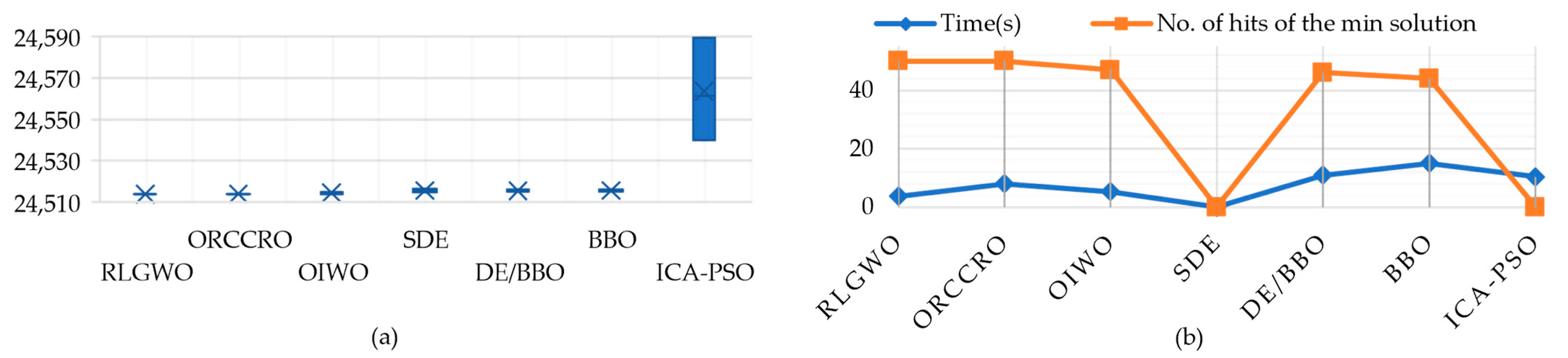
| Method | Generation Cost | Time (s) | No. of Hits of the Minimum Solution | ||
|---|---|---|---|---|---|
| Max | Min | Average | |||
| RLGWO | 24,514.78 | 24,514.78 | 24,514.78 | 3.7 | 50 |
| ORCCRO | 24,513.91 | 24,513.91 | 24,513.91 | 8 | 50 |
| OIWO | 24,514.83 | 24,514.83 | 24,514.83 | 5.3 | 47 |
| SDE | NA | 24,514.88 | 24,516.31 | NA | NA |
| DE/BBO | 24,515.98 | 24,514.97 | 24,515.05 | 11 | 46 |
| BBO | 24,516.09 | 24,515.21 | 24,515.32 | 15 | 44 |
| ICA-PSO | 24,589.45 | 24,540.06 | 24,561.46 | 10.4 | NA |
| Unit Number | Methods | ||||||
|---|---|---|---|---|---|---|---|
| RLGWO | OIWO | DE/BBO | ORCCRO | BBO | SDE | GAAPI | |
| 1 | 113.9954 | 113.9908 | 111.04 | 111.68 | 112.54 | 110.06 | 114 |
| 2 | 114 | 114 | 113.71 | 112.16 | 113.22 | 112.41 | 114 |
| 3 | 119.99885 | 119.9977 | 118.64 | 119.98 | 119.51 | 120 | 120 |
| 4 | 183.0428 | 182.5131 | 189.49 | 182.18 | 188.37 | 188.72 | 190 |
| 5 | 88.1189 | 88.4227 | 86.32 | 87.28 | 90.41 | 85.91 | 97 |
| 6 | 140 | 140 | 139.88 | 139.85 | 139.05 | 140 | 140 |
| 7 | 299.99995 | 299.9999 | 299.86 | 298.15 | 294.97 | 250.19 | 300 |
| 8 | 296.0327 | 292.0654 | 285.42 | 286.89 | 299.18 | 290.68 | 300 |
| 9 | 299.94085 | 299.8817 | 296.29 | 293.38 | 296.46 | 300 | 300 |
| 10 | 279.7137 | 279.7073 | 285.07 | 279.34 | 279.89 | 282.01 | 205.25 |
| 11 | 197.0559 | 168.8149 | 164.69 | 162.35 | 160.15 | 180.82 | 226.3 |
| 12 | 94.08905 | 94 | 94 | 94.12 | 96.74 | 168.74 | 204.72 |
| 13 | 484.1729 | 484.0758 | 486.3 | 486.44 | 484.04 | 469.96 | 346.48 |
| 14 | 484.19005 | 484.0477 | 480.7 | 487.02 | 483.32 | 484.17 | 434.32 |
| 15 | 484.044 | 484.0396 | 480.66 | 483.39 | 483.77 | 487.73 | 431.34 |
| 16 | 484.08385 | 484.0886 | 485.05 | 484.51 | 483.3 | 482.3 | 440.22 |
| 17 | 489.248 | 489.2813 | 487.94 | 494.22 | 490.83 | 499.64 | 500 |
| 18 | 489.27865 | 489.2966 | 491.09 | 489.48 | 492.19 | 411.32 | 500 |
| 19 | 511.328 | 511.3219 | 511.79 | 512.2 | 511.28 | 510.47 | 550 |
| 20 | 511.41705 | 511.335 | 544.89 | 513.13 | 521.55 | 542.04 | 550 |
| 21 | 536.7086 | 549.9412 | 528.92 | 543.85 | 526.42 | 544.81 | 550 |
| 22 | 548.3222 | 549.9999 | 540.58 | 548 | 538.3 | 550 | 550 |
| 23 | 523.33305 | 523.2804 | 524.98 | 521.21 | 534.74 | 550 | 550 |
| 24 | 523.32785 | 523.3213 | 524.12 | 525.01 | 521.2 | 528.16 | 550 |
| 25 | 523.4937 | 523.5804 | 534.49 | 529.84 | 526.14 | 524.16 | 550 |
| 26 | 523.44335 | 523.5847 | 529.15 | 540.04 | 544.43 | 539.1 | 550 |
| 27 | 10.0081 | 10.0086 | 10.51 | 12.59 | 11.51 | 10 | 11.44 |
| 28 | 10.0086 | 10.0068 | 10 | 10.06 | 10.21 | 10.37 | 11.56 |
| 29 | 10.03725 | 10.0123 | 10 | 10.79 | 10.71 | 10 | 11.42 |
| 30 | 87.83375 | 87.8664 | 90.06 | 89.7 | 88.28 | 96.1 | 97 |
| 31 | 190 | 190 | 189.82 | 189.59 | 189.84 | 185.33 | 190 |
| 32 | 189.99915 | 189.9983 | 187.69 | 189.96 | 189.94 | 189.54 | 190 |
| 33 | 190 | 190 | 189.97 | 187.61 | 189.13 | 189.96 | 190 |
| 34 | 199.997 | 199.994 | 199.83 | 198.91 | 198.07 | 199.9 | 200 |
| 35 | 200 | 200 | 199.93 | 199.98 | 199.92 | 196.25 | 200 |
| 36 | 164.86345 | 164.8283 | 163.03 | 165.68 | 194.35 | 185.85 | 200 |
| 37 | 110 | 110 | 109.85 | 109.98 | 109.43 | 109.72 | 110 |
| 38 | 109.997 | 109.994 | 109.26 | 109.82 | 109.56 | 110 | 110 |
| 39 | 110 | 110 | 109.6 | 109.88 | 109.62 | 95.71 | 110 |
| 40 | 530.92635 | 550 | 543.23 | 548.5 | 527.82 | 532.43 | 550 |
| Total generating output | 11,456.05 | 11,457.2965 | 11,457.83 | 11,458.75 | 11,470 | 11,474.43 | 11,545.06 |
| Power loss | 956.05 | 957.2965 | 957.83 | 958.75 | 970.37 | 974.43 | 1045.06 |
| Fuel cost | 136,548.3499 | 136,452.677 | 136,950.77 | 136,855.19 | 137,026.82 | 138,157.46 | 139,864.96 |
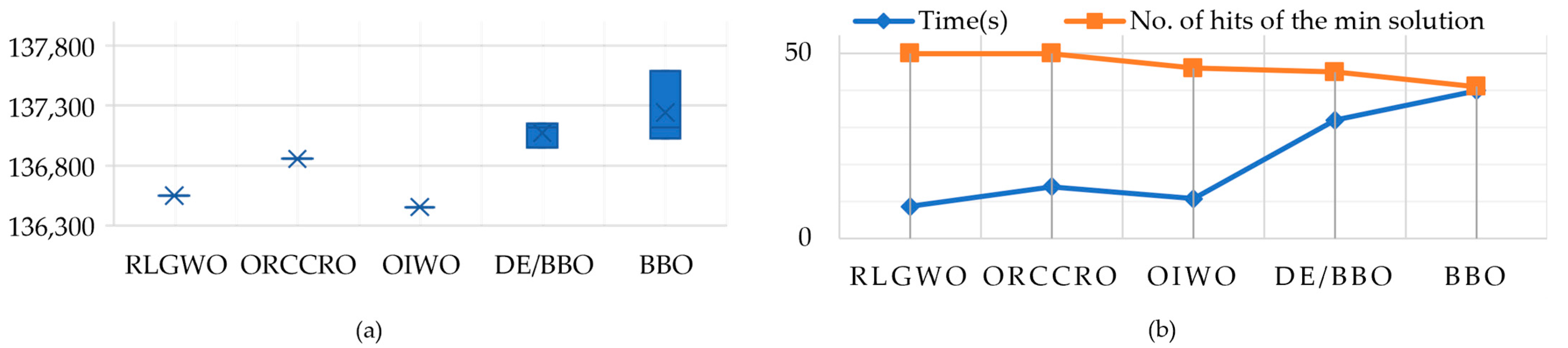
| Method | Generation Costs | Time (s) | No. of Hits of the Minimum Solution | ||
|---|---|---|---|---|---|
| Max | Min | Average | |||
| RLGWO | 136,548.3499 | 136,548.3499 | 136,548.3499 | 8.6 | 50 |
| ORCCRO | 136,855.19 | 136,855.19 | 136,855.19 | 14 | 50 |
| OIWO | 136,452.677 | 136,452.677 | 136,452.677 | 10.7 | 46 |
| DE/BBO | 137,150.77 | 136,950.77 | 137,116.58 | 32 | 45 |
| BBO | 137,587.82 | 137,026.82 | 137,116.58 | 40 | 41 |
| Unit | Power Output (MW) | Unit | Power Output (MW) | Unit | Power Output (MW) | Unit | Power Output (MW) | Unit | Power Output (MW) |
|---|---|---|---|---|---|---|---|---|---|
| 1 | 2.34 | 24 | 350.0000 | 47 | 5.4008 | 70 | 360.0000 | 93 | 440.0000 |
| 2 | 2.3985 | 25 | 400.0000 | 48 | 5.4000 | 71 | 400.0000 | 94 | 499.972 |
| 3 | 2.3985 | 26 | 400.0000 | 49 | 8.4012 | 72 | 400.0000 | 95 | 600.0000 |
| 4 | 2.3991 | 27 | 499.9991 | 50 | 8.4000 | 73 | 107.8423 | 96 | 469.2669 |
| 5 | 2.3991 | 28 | 500.0000 | 51 | 8.4000 | 74 | 188.8107 | 97 | 3.6000 |
| 6 | 4.0006 | 29 | 199.9902 | 52 | 12.0000 | 75 | 89.9956 | 98 | 3.6000 |
| 7 | 4.0000 | 30 | 99.9986 | 53 | 12.0000 | 76 | 49.9991 | 99 | 4.4000 |
| 8 | 4.0000 | 31 | 10.0003 | 54 | 12.008 | 77 | 160.0137 | 100 | 4.4002 |
| 9 | 4.0000 | 32 | 19.9852 | 55 | 12.0006 | 78 | 291.3489 | 101 | 10.0075 |
| 10 | 63.0201 | 33 | 79.4518 | 56 | 25.2000 | 79 | 176.9972 | 102 | 10.003 |
| 11 | 59.2256 | 34 | 250.0000 | 57 | 25.2000 | 80 | 97.7541 | 103 | 20.0037 |
| 12 | 35.5324 | 35 | 359.9998 | 58 | 35.0000 | 81 | 10.0007 | 104 | 20.0036 |
| 13 | 57.4253 | 36 | 399.9929 | 59 | 35.0000 | 82 | 12.3103 | 105 | 40.0000 |
| 14 | 25.0000 | 37 | 39.9998 | 60 | 45.0013 | 83 | 20.0453 | 106 | 40.0011 |
| 15 | 25.0000 | 38 | 69.9965 | 61 | 45.0013 | 84 | 199.9869 | 107 | 50.0000 |
| 16 | 25.00011 | 39 | 99.9896 | 62 | 45.0000 | 85 | 324.5166 | 108 | 30.0000 |
| 17 | 155.0000 | 40 | 120.0000 | 63 | 184.9962 | 86 | 439.9885 | 109 | 40.0000 |
| 18 | 155.0000 | 41 | 156.8012 | 64 | 184.9953 | 87 | 18.8657 | 110 | 20.0000 |
| 19 | 155.0000 | 42 | 219.9997 | 65 | 184.9997 | 88 | 23.3351 | Fuel Cost ($/h) | 197,952.36 |
| 20 | 154.9936 | 43 | 440.0000 | 66 | 185.0000 | 89 | 84.4017 | ||
| 21 | 68.89 | 44 | 560.0000 | 67 | 70.0000 | 90 | 91.9005 | ||
| 22 | 68.89 | 45 | 660.0000 | 68 | 70.0000 | 91 | 58.2891 | ||
| 23 | 68.89 | 46 | 619.5389 | 69 | 70.0006 | 92 | 98.38849 |
| Method | Generation Costs | Time (s) | No. of Hits of the Minimum Solution | ||
|---|---|---|---|---|---|
| Max | Min | Average | |||
| RLGWO | 197,952.88 | 197,952.36 | 197,952.62 | 28 | 49 |
| ORCCRO | 198,016.89 | 198,016.29 | 198,016.32 | 45 | 48 |
| OIWO | 197,989.93 | 197,989.14 | 197,989.41 | 31 | 46 |
| DE/BBO | 198,828.57 | 198,231.06 | 198,326.66 | 132 | 43 |
| BBO | 199,102.59 | 198,241.166 | 198,413.45 | 115 | 41 |
| Unit | Power Output (MW) | Unit | Power Output (MW) | Unit | Power Output (MW) | Unit | Power Output (MW) | Unit | Power Output (MW) |
|---|---|---|---|---|---|---|---|---|---|
| 1 | 116.74945 | 29 | 501 | 57 | 103 | 85 | 115 | 113 | 94 |
| 2 | 189 | 30 | 501 | 58 | 198 | 86 | 207 | 114 | 94 |
| 3 | 190 | 31 | 506 | 59 | 312 | 87 | 207 | 115 | 244 |
| 4 | 190 | 32 | 506 | 60 | 281.8723 | 88 | 175 | 116 | 244 |
| 5 | 168.53975 | 33 | 506 | 61 | 163 | 89 | 175 | 117 | 244 |
| 6 | 190 | 34 | 506 | 62 | 95 | 90 | 175 | 118 | 95 |
| 7 | 490 | 35 | 500 | 63 | 160.442 | 91 | 175 | 119 | 95 |
| 8 | 490 | 36 | 500 | 64 | 160 | 92 | 580 | 120 | 116 |
| 9 | 496 | 37 | 241 | 65 | 490 | 93 | 645 | 121 | 175 |
| 10 | 496 | 38 | 241 | 66 | 196.13105 | 94 | 984 | 122 | 2 |
| 11 | 496 | 39 | 774 | 67 | 490 | 95 | 978 | 123 | 4 |
| 12 | 496 | 40 | 769 | 68 | 489.80065 | 96 | 682 | 124 | 15 |
| 13 | 506 | 41 | 3 | 69 | 130 | 97 | 720 | 125 | 9 |
| 14 | 509 | 42 | 3 | 70 | 234.70625 | 98 | 718 | 126 | 12 |
| 15 | 506 | 43 | 250 | 71 | 137 | 99 | 720 | 127 | 10 |
| 16 | 505 | 44 | 248.19195 | 72 | 325.6586 | 100 | 964 | 128 | 112 |
| 17 | 506 | 45 | 250 | 73 | 195 | 101 | 958 | 129 | 4 |
| 18 | 506 | 46 | 250 | 74 | 175.3892 | 102 | 1007 | 130 | 5 |
| 19 | 505 | 47 | 245.45 | 75 | 175 | 103 | 1006 | 131 | 5 |
| 20 | 505 | 48 | 250 | 76 | 175.9936 | 104 | 1013 | 132 | 50 |
| 21 | 505 | 49 | 250 | 77 | 175.4087 | 105 | 1020 | 133 | 5 |
| 22 | 505 | 50 | 250 | 78 | 330 | 106 | 954 | 134 | 42 |
| 23 | 505 | 51 | 165 | 79 | 531 | 107 | 952 | 135 | 42 |
| 24 | 505 | 52 | 165 | 80 | 531 | 108 | 1006 | 136 | 41 |
| 25 | 537 | 53 | 165 | 81 | 382.3908 | 109 | 1013 | 137 | 17 |
| 26 | 537 | 54 | 165 | 82 | 56 | 110 | 1021 | 138 | 11.211 |
| 27 | 549 | 55 | 180 | 83 | 115 | 111 | 1015 | 139 | 7 |
| 28 | 549 | 56 | 180 | 84 | 115 | 112 | 94 | 140 | 26.06515 |
| Fuel Cost ($/h) = 1,559,390 | Load demand = 49,342 MW | ||||||||
| Method | Generation Costs | Time (s) | No. of Hits of the Minimum Solution | ||
|---|---|---|---|---|---|
| Max | Min | Average | |||
| RLGWO | 1,559,389.896 | 1,559,389.595 | 1,559,389.746 | 44.2 | 49 |
| OIWO | 1,559,405.88 | 1,559,405.45 | 1,559,405.61 | 46.8 | 46 |
| Unit | Power Output (MW) | Unit | Power Output (MW) | Unit | Power Output (MW) | Unit | Power Output (MW) | Unit | Power Output (MW) | Unit | Power Output (MW) |
|---|---|---|---|---|---|---|---|---|---|---|---|
| 1 | 221.00035 | 28 | 231.8196 | 55 | 270.9179 | 82 | 201.35535 | 109 | 430.44955 | 136 | 237.9752 |
| 2 | 205.7281 | 29 | 425.93425 | 56 | 248.48075 | 83 | 314.73155 | 110 | 269.64185 | 137 | 295.55395 |
| 3 | 317.75575 | 30 | 279.58085 | 57 | 281.2539 | 84 | 237.5059 | 111 | 217.76425 | 138 | 235.6813 |
| 4 | 234.41735 | 31 | 196.63605 | 58 | 238.18815 | 85 | 275.93495 | 112 | 205.1143 | 139 | 430.2502 |
| 5 | 2912142 | 32 | 207.35155 | 59 | 412.3851 | 86 | 224.36975 | 113 | 318.7791 | 140 | 268.2663 |
| 6 | 244.9315 | 33 | 314.11745 | 60 | 278.72325 | 87 | 284.14205 | 114 | 245.6407 | 141 | 223.00885 |
| 7 | 297.5845 | 34 | 229.92935 | 61 | 229.1329 | 88 | 247.8263 | 115 | 271.79755 | 142 | 197.70995 |
| 8 | 229.63355 | 35 | 280.2443 | 62 | 212.27065 | 89 | 419.6053 | 116 | 246.03355 | 143 | 325.12455 |
| 9 | 382.95085 | 36 | 242.2372 | 63 | 310.3729 | 90 | 274.05395 | 117 | 288.0778 | 144 | 229.6929 |
| 10 | 274.7838 | 37 | 299.5748 | 64 | 244.48875 | 91 | 205.04785 | 118 | 237.1986 | 145 | 270.23625 |
| 11 | 202.63435 | 38 | 238.49285 | 65 | 254.77565 | 92 | 206.14835 | 119 | 379.98875 | 146 | 237.61965 |
| 12 | 203.3912 | 39 | 385.28865 | 66 | 242.9497 | 93 | 315.2499 | 120 | 289.60535 | 147 | 293.18245 |
| 13 | 316.69635 | 40 | 306.1279 | 67 | 297.698 | 94 | 249.54195 | 121 | 227.5547 | 148 | 241.3283 |
| 14 | 240.61475 | 41 | 223.84795 | 68 | 236.58335 | 95 | 283.55655 | 122 | 209.27635 | 149 | 408.69515 |
| 15 | 274.9389 | 42 | 210.5801 | 69 | 391.7068 | 96 | 233.38845 | 123 | 308.35835 | 150 | 273.40185 |
| 16 | 234.0219 | 43 | 310.6721 | 70 | 280.0213 | 97 | 292.58485 | 124 | 225.3519 | 151 | 201.19515 |
| 17 | 281.37655 | 44 | 236.8065 | 71 | 218.70865 | 98 | 232.1082 | 125 | 258.85355 | 152 | 211.8315 |
| 18 | 232.42195 | 45 | 288.09185 | 72 | 215.8047 | 99 | 398.45225 | 126 | 243.2848 | 153 | 328.14365 |
| 19 | 417.2048 | 46 | 251.70135 | 73 | 311.6729 | 100 | 283.92175 | 127 | 289.6619 | 154 | 244.37645 |
| 20 | 296.69975 | 47 | 264.1946 | 74 | 245.34615 | 101 | 222.28885 | 128 | 243.20055 | 155 | 277.40895 |
| 21 | 211.53615 | 48 | 226.43815 | 75 | 274.99975 | 102 | 211.05235 | 129 | 430.75805 | 156 | 231.75945 |
| 22 | 205.97795 | 49 | 396.5202 | 76 | 228.8927 | 103 | 321.53435 | 130 | 263.69975 | 157 | 274.733 |
| 23 | 327.2297 | 50 | 291.1473 | 77 | 295.2527 | 104 | 231.10145 | 131 | 208.5112 | 158 | 237.31805 |
| 24 | 237.09925 | 51 | 199.54815 | 78 | 242.0892 | 105 | 255.53405 | 132 | 214.2303 | 159 | 410.52905 |
| 25 | 280.7248 | 52 | 211.2342 | 79 | 391.79425 | 106 | 236.2335 | 133 | 310.9484 | 160 | 282.7046 |
| 26 | 230.7831 | 53 | 322.1792 | 80 | 275.43885 | 107 | 283.8343 | 134 | 234.9219 | Fuel Cost (S/h) | 9914.7123 |
| 27 | 269.3144 | 54 | 237.0891 | 81 | 220.4749 | 108 | 238.32985 | 135 | 263.6612 |
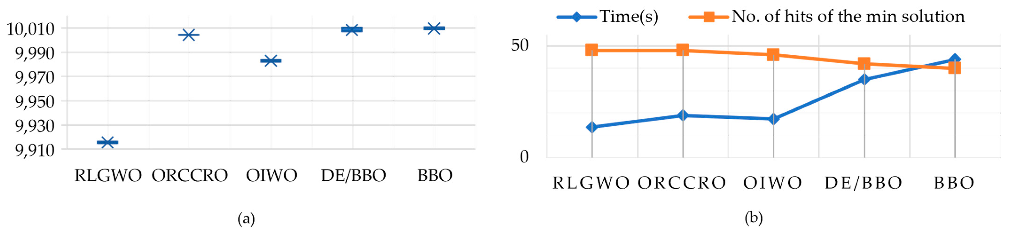
| Method | Generation Costs | Time (s) | No. of Hits of the Minimum Solution | ||
|---|---|---|---|---|---|
| Max | Min | Average | |||
| RLGWO | 9916.4457 | 9914.7123 | 9915.579 | 13.7 | 48 |
| ORCCRO | 10,004.45 | 10,004.2 | 10,004.21 | 19 | 48 |
| OIWO | 9983.998 | 9981.9834 | 9982.991 | 17.3 | 46 |
| DE/BBO | 10,010.25 | 10,007.05 | 10,007.56 | 35 | 42 |
| BBO | 10,010.59 | 10,008.71 | 10,009.16 | 44 | 40 |
Disclaimer/Publisher’s Note: The statements, opinions and data contained in all publications are solely those of the individual author(s) and contributor(s) and not of MDPI and/or the editor(s). MDPI and/or the editor(s) disclaim responsibility for any injury to people or property resulting from any ideas, methods, instructions or products referred to in the content. |
© 2023 by the authors. Licensee MDPI, Basel, Switzerland. This article is an open access article distributed under the terms and conditions of the Creative Commons Attribution (CC BY) license (https://creativecommons.org/licenses/by/4.0/).
Share and Cite
Tai, T.-C.; Lee, C.-C.; Kuo, C.-C. A Hybrid Grey Wolf Optimization Algorithm Using Robust Learning Mechanism for Large Scale Economic Load Dispatch with Vale-Point Effect. Appl. Sci. 2023, 13, 2727. https://doi.org/10.3390/app13042727
Tai T-C, Lee C-C, Kuo C-C. A Hybrid Grey Wolf Optimization Algorithm Using Robust Learning Mechanism for Large Scale Economic Load Dispatch with Vale-Point Effect. Applied Sciences. 2023; 13(4):2727. https://doi.org/10.3390/app13042727
Chicago/Turabian StyleTai, Tzu-Ching, Chen-Cheng Lee, and Cheng-Chien Kuo. 2023. "A Hybrid Grey Wolf Optimization Algorithm Using Robust Learning Mechanism for Large Scale Economic Load Dispatch with Vale-Point Effect" Applied Sciences 13, no. 4: 2727. https://doi.org/10.3390/app13042727
APA StyleTai, T.-C., Lee, C.-C., & Kuo, C.-C. (2023). A Hybrid Grey Wolf Optimization Algorithm Using Robust Learning Mechanism for Large Scale Economic Load Dispatch with Vale-Point Effect. Applied Sciences, 13(4), 2727. https://doi.org/10.3390/app13042727