A Computationally Efficient Algorithm for Feedforward Active Noise Control Systems

Abstract

In this paper, a novel algorithm with high computational efficiency is proposed for the filter adaptation in a feedforward active noise control system. The proposed algorithm Zero Forcing Block Adaptive Filter (ZF-BAF) performs filter adaptation on a block-by-block basis in the frequency domain. Filtering is performed in the time domain on a sample-by-sample basis. Working in the frequency domain permits us to get sub-linear complexity, whereas filtering in the time domain minimizes the latency. Furthermore, computational burden is tunable to meet specific requirements about adaptation speed and processing load. No other parameter tuning according to the working condition is required. Computer simulations, performed in different realistic cases against other high-performing time and frequency-domain algorithms, show that achievable performances are comparable, or even better, with those of the algorithms perfectly tuned for each specific case. Robustness exhibited in the tests suggests that performances are expected to be even better in a wide range of real cases where it is impossible to know a priori how to tune the algorithms.

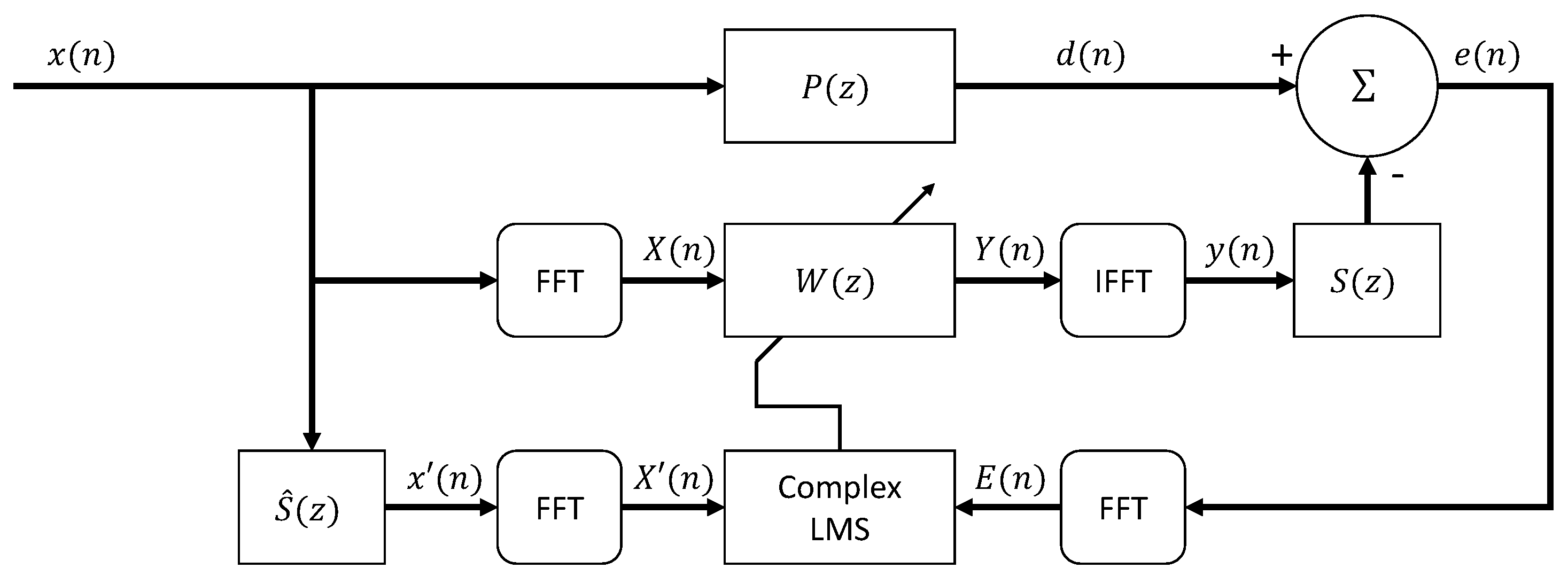
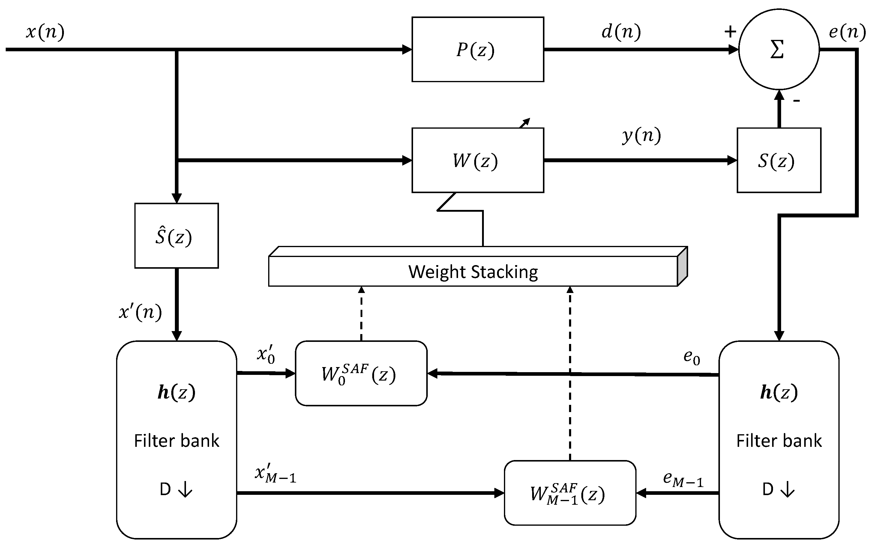
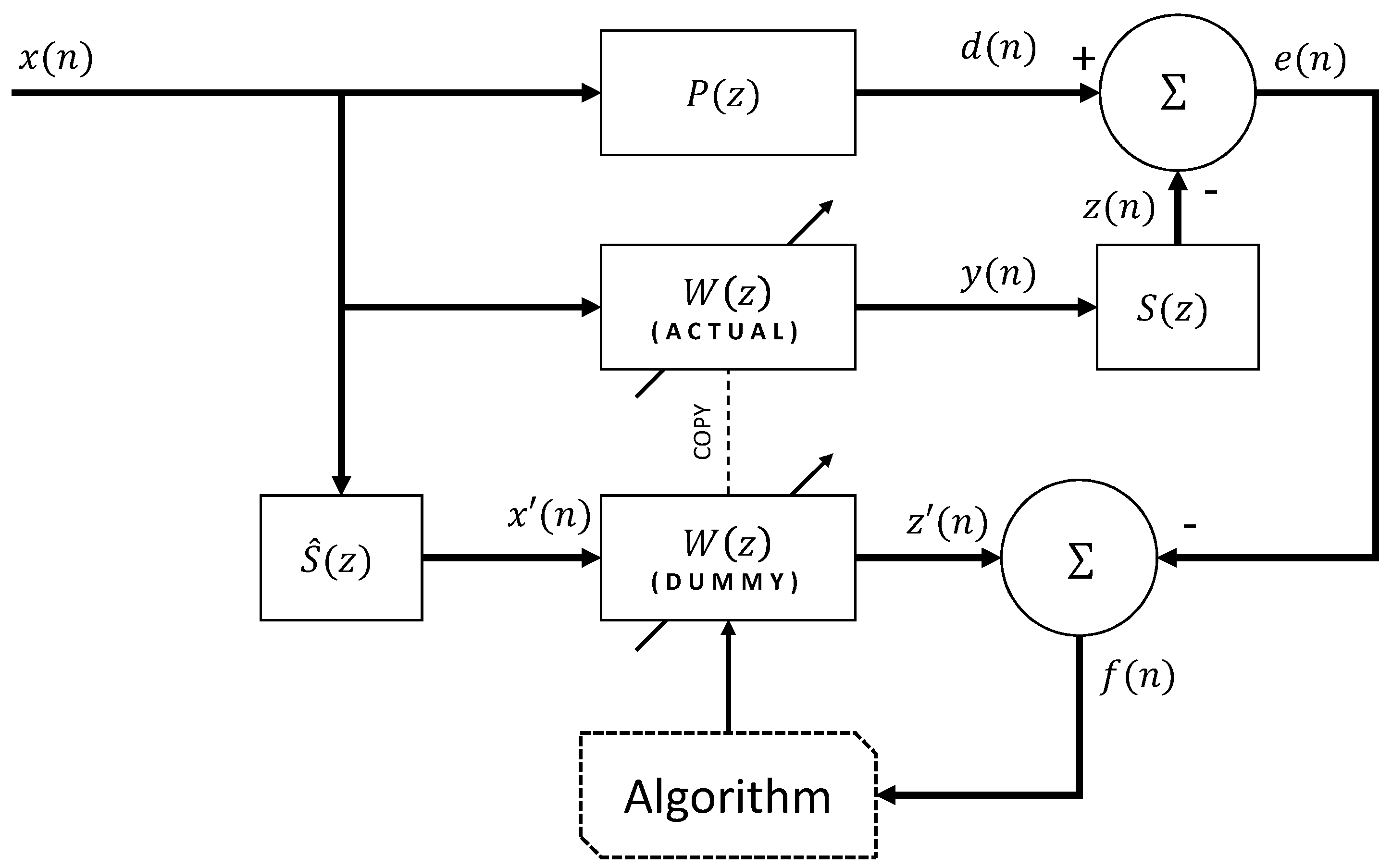
1. Introduction

Noise cancellation encompass all the techniques that are able to remove unwanted noise given a signal affected by it. Two major families of noise cancellation techniques exist: passive noise cancellation and active noise cancellation. The former involves the presence of a passive filter (either analog or digital [1,2]) operating on the noisy signal. This methodology, although simple in practice, can be implemented in very complex fashions, involving sub-band adaptive filtering [3] or machine-learning-based techniques [4,5]. Moreover, it is often a very convenient solution in electronic power systems for Electro-Magnetic Interferece (EMI) filtering [6,7] The latter, Active Noise Cancellation (ANC) is a technique that, by processing two signals, namely a reference signal and an error signal, by means of adaptive filtering, produces another signal, named antinoise, that reduces the level of an undesired noise [8,9,10]. This technique finds usage in different fields of application where the reduction of unwanted noise is desirable. Notable examples include automotive [11,12], biomedical [13], power [14,15] and aerospace [16] engineering. Moreover, this technology reached a maturity level for consumer application such as noise canceling headphones [17,18], aid devices [19], and welcomes novel numerical techniques such as neural networks [20]. A duct-noise cancellation system based on adaptive filter theory was developed by Burgess in [21].

Indeed, the application field for these kinds of algorithms is very large, both in terms of physical systems and hardware resources. For this reason, the qualities of efficiency (in terms of computational costs), effectiveness (in terms of noise reduction) and robustness (in terms of flexibility with respect to sudden changes in the system) are of paramount importance when designing an ANC algorithm. Moreover, simplicity of a minimum tuning paradigm and set-up effort are desirable. In general, realistic ANC applications features paths with very long impulse response. The adaptive filters used for noise cancellation inherit this length and, for this reason, the signal processing part of the algorithm suffers from an elevated computational cost. To reduce such costs, the problem is often approached in the frequency domain. In the frequency domain, the signals are decomposed and processed in individual blocks by means of specific filter banks. Algorithms such as the ones presented in [22,23,24,25,26] are all valid implementations for frequency-domain ANC. Authors in [24,25] propose an algorithm that features computational advantages by performing all the signal processing in the frequency domain, thus accelerating the algorithm for large filter-order L. With this approach, although the control filter is adapted every L samples, instead of every sample as with conventional time-domain adaptive filters, the filter coefficients are adapted with greater precision.

An ANC system using a Frequency-domain Filtered-x Least Mean Squares (FxLMS) algorithm is illustrated in Figure 1. This approach has the advantage of reducing the computational costs involved while preserving the performance in noise reduction. However, the length for the signal path delay corresponds to one block. A variation of the block transform approach that eliminates signal path delay has been proposed in [27,28] for an acoustic echo canceler. Moreover, the authors of [29] proposed in their work a Block Adaptive Filtering algorithm (BAF), based on Discrete Fourier Transform (DFT) Multidelay Adaptive Filter (DFT-MDF). The algorithm implements structures based on strictly real arithmetic, resulting in a leaner signal processing implementation with higher computational performance. The algorithm proposed in [29] can be generalized towards Subband Adaptive Filtering (SAF) techniques, such as the ones in [3,30], and notably [31] for MIMO scenarios. The SAF algorithms, whose block diagram is reported in Figure 2, make use of decomposition of reference and error signals in subbands by means of filter banks. Signal decomposition in subbands makes it possible to use the time domain FxLMS algorithm in each of these working at a lower frequency sample. All subbands in the control filter are then arranged together to realize the control filter. Since filter bank can be efficiently implemented exploiting the FFT algorithm and since each FxLMS works at a lower frequency rate, efficient implementations are possible.

Among the SAF methods, the delayless SAF introduced by [32] provides a better approach to meet the computational requirements for ANC system. Tuning of the SAF algorithm can be very difficult [33], and the one proposed by [34] achieves a reduction of spectral leakage by applying a decimation factor and a proper weight stacking methodology, resulting in an SAF algorithm with very low computational complexity without degrading the ANC performance. This algorithm is going to be used as standard comparison to validate the computational complexity and performance of the algorithm herein proposed.

The algorithm ZF-BAF (Zero Forcing Block Adaptive Filter) proposed in this work aims at solving the problem of updating the adaptation filter W periodically in the frequency domain, weighting each component of the filter by means of spectral characteristics of the noise vector. Since the adaptation of the filter is done in the frequency domain, the computational load is reduced to sub-linear complexity. Filtering, on the other hand, is performed in the time domain, achieving low latency.

The paper will be structured as follows. In the first part, the general ANC system will be briefly described, and the proposed algorithm will be described step-by-step. Following, the computational costs for the algorithm will be thoroughly discussed. A comprehensive validation of the proposed algorithm through simulations will be presented in the results section. Conclusions and final remarks will close the paper.

2. Materials and Methods

To describe the proposed ZF-BAF algorithm, let us refer to Figure 3 which reports the block diagram of a feedforward ANC system using the FxLMS algorithm (Burgess [21] and Morgan [35]). At each step n, this algorithm adjusts the coefficient vector $\mathbf{w}\left(n\right)={[w_0\left(n\right),\dots ,w_{L-1}\left(n\right)]}^T$ of the filter $W\left(z\right)$ in order to minimize the power of the error signal $e\left(n\right)$.

A different way to see this system is that in Figure 4, where the filter $W\left(z\right)$ is adjusted to generate an output $z^{\prime }\left(n\right)$ as similar as possible to the residual noise $e\left(n\right)$ when its input is $x^{\prime }\left(n\right)$.

Instead of adjusting the filter $W\left(z\right)$ at each step n, we propose here to do it on a block-by-block basis, generating an update of $W\left(z\right)$ every K samples processing the vectors ${\mathbf{x}}^{\prime }\left(n\right)={[x^{\prime }\left(n\right),\dots ,x^{\prime }(n-N+1)]}^T$ and $\mathbf{e}\left(n\right)={[e\left(n\right),\dots ,e(n-N+1)]}^T$, when n assumes the values $K,2K,\dots$

N is the length of the analysis frame. In principle, it could be grater than the filter length L. It is assumed that $x\left(n\right)=e\left(n\right)=0$ when $n<0$. Initially it is supposed that $\mathbf{w}\left(0\right)=\mathbf{0}$, therefore, when $n=K$, $\mathbf{e}\left(n\right)$ is equivalent to $\mathbf{d}\left(n\right)={[d\left(n\right),\dots ,d(n-N+1)]}^T$.

The task to be performed is to produce an update $\Delta {\mathbf{w}}_i$ of $\mathbf{w}\left(n\right)$, where $i=\left[n/K\right]$. Assuming that the signal $x\left(n\right)$ is slowly changing, and therefore optimal $W\left(z\right)$ as well, the vector $\mathbf{w}\left(n\right)$ will be used to generate $\mathbf{y}\left(n\right)={[y\left(n\right),\dots ,y(n-K+1)]}^T$ in the next block.

After the first $W\left(z\right)$ update, $y\prime \left(n\right)$ is present affecting $e\left(n\right)$. After other K samples ($i=2$), another $W\left(z\right)$ update, namely $\Delta {\mathbf{w}}_2\left(n\right)$, is expected. This update could be thought of as the filter that, when its input is ${\mathbf{x}}^{\prime }\left(2K\right)$, produces the vector $\mathbf{e}\left(2K\right)$ as output.

In the end, at each block i, the problem to solve is always to find the coefficients $\Delta {\mathbf{w}}_i$ of $W\left(z\right)$ that should have minimized the difference between filter output $z^{\prime }\left(n\right)$ and the error $e\left(n\right)$ during the last N samples.

Adjustments of $W\left(z\right)$ are performed every K samples, but the output $y\left(n\right)$ is produced on a sample-by-sample basis.

In this paper, we propose to solve this problem in the frequency domain. Since the output of the filter is $Z^{\prime }\left(z\right)=W\left(z\right)X^{\prime }\left(z\right)$, the adjustments $\Delta {\mathbf{w}}_i$ for $\mathbf{w}\left(n\right)$ able to generate $E\left(z\right)$, can be obtained by:

$$\Delta W_i\left(l\right)=\frac{E_i\left(l\right)}{X_i^{\prime }\left(l\right)}l=0,\dots ,N-1.$$

(1)

where the terms $X_i^{\prime }\left(l\right)$ and $E_i\left(l\right)$ stands, respectively, for the $l_{th}$ discrete Fourier transforms (DFT) coefficient of the vectors ${\mathbf{x}}^{\prime }\left(n\right)$ and $\mathbf{e}\left(n\right)$ (which are supposed to be known for this algorithmic approach). The technique proposed is based on the zero forcing equalizer presented in [36].

If $W_i\left(l\right)$ is the DFT of the filter coefficients vector $\mathbf{w}\left(n\right)$ employed in the current analysis frame, that of the vector $\mathbf{w}\left(n\right)$ that will be used in the next one, namely $W_{i+1}\left(l\right)$, is given by the following:

$$W_{i+1}\left(l\right)=W_i+\frac{E_i\left(l\right)}{X_i^{\prime }\left(l\right)}l=0,\dots ,N-1.$$

(2)

This approach, however, could give a too-high gain for those frequencies that have very low $\left|X_i^{\prime }\left(l\right)\right|$. To avoid this, it was preferred to limit $W\left(z\right)$ to depends only on the phase of $X\left(l\right)$, but not on its module, that is:

$$W_{i+1}\left(l\right)=W_i+G\left(n\right)·E_i\left(l\right)\frac{\left|X_i^{\prime }\left(l\right)\right|}{X_i^{\prime }\left(l\right)}l=0,\dots ,N-1.$$

(3)

where $G\left(n\right)$ is a gain that needs to be defined to avoid instability. If the gain is over unity for any frequency, the loop becomes unstable. This task is quite critical, since the speed of convergence and the power of the residual noise depend on it. First of all, $G\left(n\right)$ should guarantee that the power of filter output $\Delta Z^{\prime }\left(l\right)$ is at most equal to that of the residual noise $E\left(l\right)$ at each frequency $l=0,\dots ,L-1$, that is:

$$G{\left(n\right)}^2{\left|E_i\left(l\right)\right|}^2{\left|X_i^{\prime }\left(l\right)\right|}^2<{\left|E_i\left(l\right)\right|}^{2}l=0,\dots ,N-1$$

(4)

that means:

$$G{\left(n\right)}^2<\frac{1}{{\left|X_i^{\prime }\left(l\right)\right|}^2}l=0,\dots ,N-1$$

(5)

The following condition guarantees the previous one:

$$G{\left(n\right)}^2\sum _{l=0}^{N-1}{\left|X_i^{\prime }\left(l\right)\right|}^2=1$$

(6)

because

$$G{\left(n\right)}^2=\frac{1}{{\sum }_{l=0}^{N-1}{\left|X_i^{\prime }\left(l\right)\right|}^2}<\frac{1}{{\left|X_i^{\prime }\left(l\right)\right|}^2}l=0,\dots ,N-1$$

(7)

Recalling now the Parseval theorem:

$$G\left(n\right)=\frac{1}{\sqrt{{\sum }_{i=0}^{N-1}{\left|X_i^{\prime }\left(l\right)\right|}^2}}=\frac{1}{N\sqrt{P_{x^{\prime }}\left(n\right)}},$$

(8)

where $P_{x^{\prime }}\left(n\right)$, the power of $x^{\prime }\left(n\right)$ in the current frame, could also be calculated in the time domain as:

$$P_{x^{\prime }}\left(n\right)=\frac{1}{N}·\sum _{i=0}^{N-1}{x^{\prime }}^2(n-i).$$

(9)

At each block i, therefore, the adjustment to apply to the vector $\mathbf{w}\left(n\right)$ is given by:

$$\Delta W_i\left(l\right)=\frac{E\left(l\right)}{X_i^{\prime }\left(l\right)}·\frac{\left|X_i^{\prime }\left(l\right)\right|}{N\sqrt{P_{x^{\prime }}\left(n\right)}}l=0,\dots ,N-1$$

(10)

After having calculated $\Delta {\mathbf{W}}_i={\left[\Delta W_i\left(l\right),\dots ,\Delta W_i(N-1))\right]}^T$, the adjustment for the coefficient vector of $W\left(z\right)$ is simply given by the inverse Fourier transform of $\Delta \mathbf{W}$:

$$\Delta \mathbf{w}\left(n\right)={\mathrm{DFT}}^{-1}(\Delta {\mathbf{W}}_i).$$

(11)

Experimentally, it was found that the minimum frame length to have a stable behavior is $N=2L$, using only the first L elements of $\Delta \mathbf{w}\left(n\right)$ to adapt $\mathbf{w}\left(n\right)$, as in the following:

$$w\left(i\right)=w\left(i\right)+\Re \left[\Delta w\left(i\right)\right]l=0,\dots ,L-1,$$

(12)

where $w\left(i\right)$ is the i-th element of the vector $\mathbf{w}\left(n\right)$ and $\Re \left[\Delta w\left(i\right)\right]$ is the real part of the ith element of the vector $\Delta \mathbf{w}\left(n\right)$. Since $x\left(n\right)$ and $e\left(n\right)$ are real signals, $\Delta \mathbf{W}$ is real as well, therefore $\Im \left[\Delta w\left(i\right)\right]=0$, for $l=0,\dots ,L-1$.

Besides the length N of the analysis frame, it is required to set the adaptation frequency $f_w$, that is how many times in a second the filter $W\left(z\right)$ is adapted. The most obvious choice is to adapt $W\left(z\right)$ every $K=N$ samples, but to increase adaptation speed, or to match specific requirements on computational load, K could be less or grater than N. An adaptation rate of $f_w$ adaptations per second means to adapt the filter $W\left(z\right)$ every $K=fs/fw$ samples, where $f_s$ is the working sample frequency. It will be shown in the next paragraphs that about 30–50 adaptations per second are good enough to have the same adaptation speed of other commonly used algorithms. Summarizing, only a few steps are required to be executed every K samples of $x\left(n\right)$ and $e\left(n\right)$:

• Step 1:
  Calculate the DFTs of the vectors $\mathbf{x}\left(n\right)$ and $\mathbf{e}\left(n\right)$
• Step 2:
  Calculate $\Delta {\mathbf{W}}_i$ according to (10).
• Step 3:
  Adjust the vector $\mathbf{w}\left(n\right)$ by adding the first L elements of the inverse DFT of $\Delta {\mathbf{W}}_i$.

In Listing 1 there is a simple Matlab implementation (freely downloadable from [37]) of the proposed algorithm working in a system like that depicted in Figure 4. The output $y\left(n\right)$ is generated on a sample-by-sample basis, whereas the filter $W\left(z\right)$ is adjusted every K samples by the proposed algorithm, whose implementation is enclosed in Listing 1.

Listing 1: Matlab implementation of the proposed algorithm.

1  for n=N:NSAMPLES

2     % --- sample-by-sample time domain filtering ---

3     y(n) = x(n:−1:n−L+1)*w;

4     z(n) = y(n:−1:n−M+1)*s;

5     e(n) = d(n) − z(n);

6     Pd = lambda*Pd + (1−lambda)*d(n)^2;

7     Pe = lambda*Pe + (1−lambda)*e(n)^2;

8     a(n) = −10*log10(Pe/Pd);

9     % --- frequency domain control algorithm -------

10     if (mod(n,K)==0)

11       % input vectors

12       xvec = xx(n−N+1:n);

13       evec = e(n−N+1:n);

14       % DFTs

15       X=fft(xvec);

16       E=fft(evec);

17       % W estimation

18       Px = sum(xvec.^2)/N;

19       W = (E./X).*(abs(X))/(N*sqrt(Px));

20       % [w(0)...w(L−1)] update

21       wd = ifft(W);

21       w = w + real(wd(1:L))’;

23     end

24  end

Theory and Calculations

To evaluate the computational burden of the algorithm described above, each step presented in the previous paragraph is analyzed hereafter.

Step 1: A very efficient way to calculate the DFT of $\mathbf{x}\left(n\right)$ and $\mathbf{e}\left(n\right)$ is to use the Fast Fourier Trasform (FFT) algorithm performed on a complex vector whose real part is $\mathbf{x}\left(n\right)$ and imaginary part is $\mathbf{e}\left(n\right)$. The well-known radix-2 Cooley–Tukey [38] algorithm commonly used to calculate the FFT of a complex vector, with length N a power of 2, requires $2N{log}_2\left(N\right)$ real non-trivial multiplications, and $4N{log}_2\left(N\right)$ real additions. After that, $(N/2)·4$ additions are required in order to recover real and imaginary parts of $X\left(l\right)$ and $E\left(l\right)$.

Step 2: In this step the Expression (10) is evaluated. In order to analyze its computational burden, it is useful to rewrite the ratio between $E\left(l\right)$ and $X\left(l\right)$ separating real and imaginary parts:

$$\frac{E\left(l\right)}{X\left(l\right)}=\frac{\Re \left[X\right(l\left)\right]\ast \Re \left[E\right(l\left)\right]+\Im \left[X\right(l\left)\right]\ast \Im \left[E\right(l\left)\right]}{{\Re }^2\left[X\left(l\right)\right]+{\Im }^2\left[X\left(l\right)\right]}$$

$$+j\frac{\Im \left[E\right(l\left)\right]\ast \Re \left[X\right(l\left)\right]-\Im \left[X\right(l\left)\right]\ast \Re \left[E\right(l\left)\right]}{{\Re }^2\left[X\left(l\right)\right]+{\Im }^2\left[X\left(l\right)\right]}$$

$$l=0,\dots ,N-1.$$

(13)

Since both $x\left(n\right)$ and $e\left(n\right)$ are real vectors, their spectra are Hermitian and, as a consequence, $E\left(l\right)/X\left(l\right)$ as well. For this reason, only $N/2+1$ elements of (13) need to be evaluated, and the remaining $N/2$ elements are simply obtained by:

$$\frac{E\left(l\right)}{X\left(l\right)}=\frac{E(N-l)}{X(N-l)}l=N/2+1,\dots ,N-1.$$

(14)

In the end, it is required to perform $(N/2+1)·2$ divisions $1/x$, $(N/2+1)·6$ multiplications, and $(N/2+1)·3$ additions to calculate the ratio $E\left(l\right)/X\left(l\right)$ given by (13). After calculating this ratio, it is also required to evaluate the weighting function:

$$\frac{\left|X\left(l\right)\right|}{N\sqrt{P_x}}=\frac{\sqrt{{\Re }^2\left[X\left(l\right)\right]+{\Im }^2\left[X\left(l\right)\right]}}{N\sqrt{P_x}}l=0,\dots ,N/2.$$

(15)

The term $1/\left(N\sqrt{P_x}\right)$ needs to be calculated only once every processed block, requiring one square root, one division, and $N+1$ multiply operations every K samples.

To calculate the numerator of (15), the following approximation has been found to be good enough:

$$\sqrt{{\Re }^2\left[X\left(l\right)\right]+{\Im }^2\left[X\left(l\right)\right]}\approx \left|\Re \left[X\right(l\left)\right]\right|+\left|\Im \left[X\right(l\left)\right]\right|l=0,\dots ,N/2.$$

(16)

This operation requires only $N/2+1$ additions and N absolute value operations.

In the end, the operations required to evaluate (10) are just: $(N/2+1)\ast 2+1$ divisions $1/x$, $(N/2+1)·8$ multiplications, and $(N/2+1)·4$ additions.

Step 3: In this step it is required to evaluate the inverse Fourier transform of $W\left(f\right)$. Using again the FFT algorithm, this step requires $2N{log}_2\left(N\right)$ real multiplications, and $2N{log}_2\left(N\right)$ real additions.

Since the operations above are performed $f_w$ times in a second and since $N=2L$, at each step n the operations reported in

Table 1. Number of operations required by the proposed Zero Forcing Block Adaptive Filter (ZF-BAF) algorithm per input sample.

Operation Type	Ops. per Input Sample
$Multiplications$	$\left(\frac{f_w}{f_s}\right)\left[8L{log}_2\left(2L\right)+8L\right]$
$Additions$	$\left(\frac{f_w}{f_s}\right)\left[16L{log}_2\left(2L\right)+4L\right]$
$Divisions$	$\left(\frac{f_w}{f_s}\right)\left(2L\right)$
$Squareroots$	$\left(\frac{f_w}{f_s}\right)$

are required. Among these values, that of multiplications is the most representative and can be used to compare the proposed algorithm with other algorithms.

The adaptation rate $f_w$ should be chosen in order to get a compromise between adaptation speed and computational load, but it could also be changed dynamically. For example, it could be decreased at a steady-state condition to reduce power consumption in mobile devices or to release computational resources to other processes.

With the assumption $f_w=(f_s/L)$, the number of multiplications is approximately:

$$N_{mul}=8{log}_2\left(2L\right)+8=8{log}_2\left(4L\right).$$

(17)

It will be shown in the next paragraphs that this choice allows us to get performances that are comparable to those of other algorithms in a wide range of situations; anyway, a different value of $f_w$ could be used in order to improve speed or to reduce computational load. In the end, it is worth noticing that most of the processing required by the proposed algorithm is related to the FFT algorithm, of which is available an optimized implementation for almost any hardware platform, allowing us to easily get efficient software implementations of the whole algorithm. Considering the simple numerical nature of the proposed ZF-BAF, it is suitable for implementation in embedded environments as well as microcontroller units, FPGAs and programmable DSP. On this matter, the RAM memory footprint can be different according to the size of a float in the architecture used for the implementation. The only notable occupancy is given by the N-long complex vector of float values used to store the data to be processed. In this case, the memory footprint is going to be sizeof(float) * 2 * N.

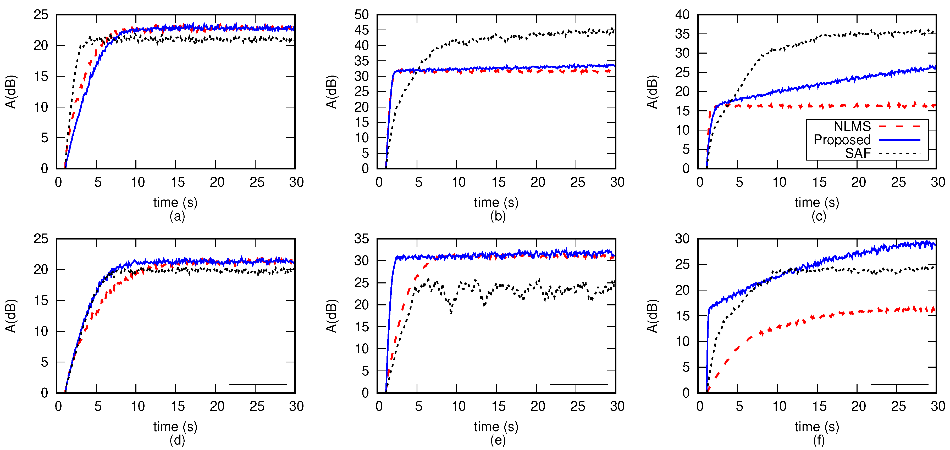
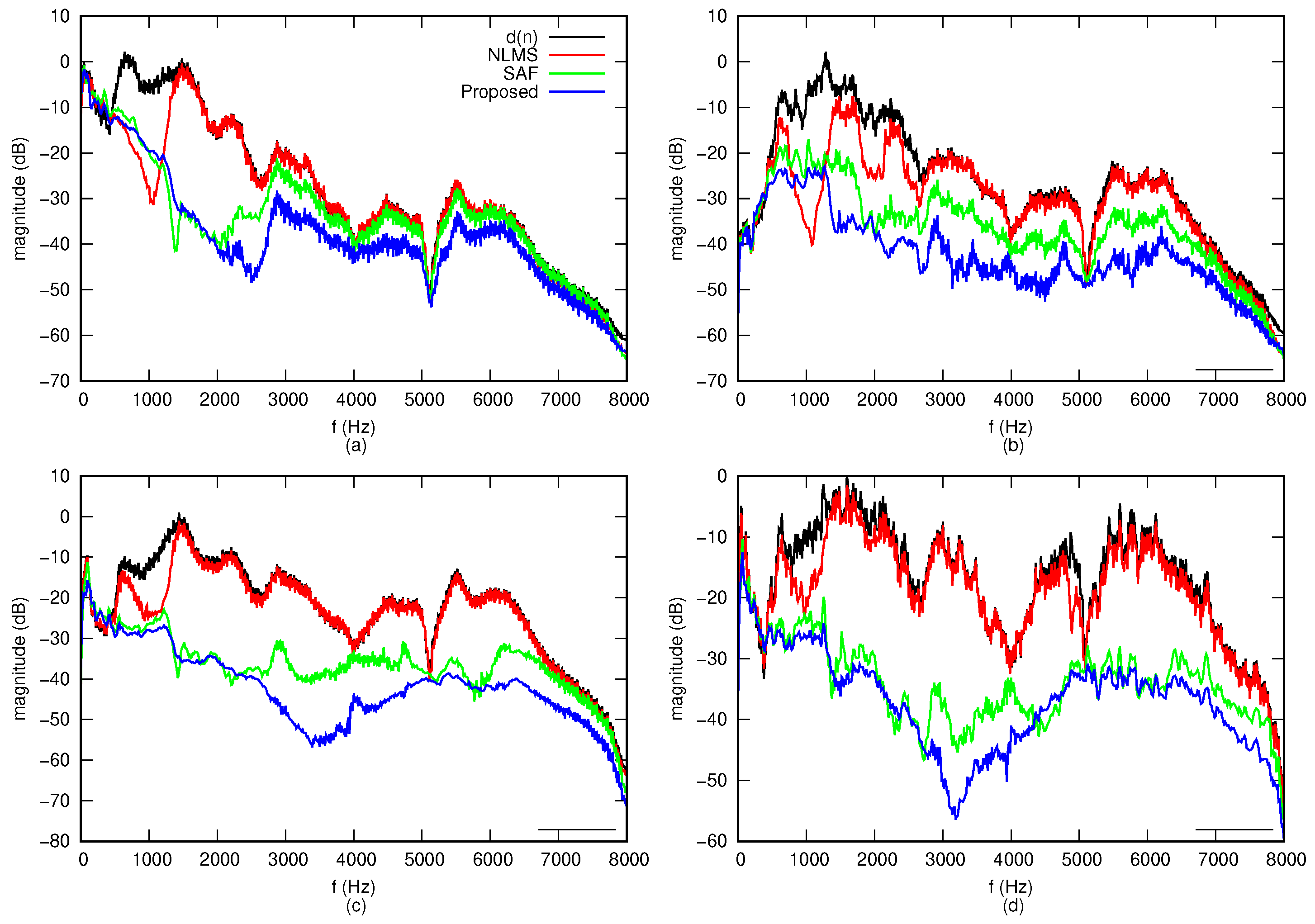
3. Results

This section describes the simulation experiments to verify the performances of the proposed ZF-BAF algorithm in a feedforward active noise control system like the one depicted in Figure 3. We investigated the ZF-BAF algorithm’s adaptation speed, noise reduction, and robustness against plant noise, different kinds of primary noise and changes in secondary paths. In these tests, the ZF-BAF algorithm is compared with the fixed step size normalized LMS (NLMS) algorithm and the SAF presented in [34]. The NLMS algorithm was chosen as adaptation algorithm in the FxLMS because it retains all the advantages of filtering the reference signal with the added benefit of normalization, which makes it less dependent on the signal power [39]. Concerning the SAF, it was chosen to have a comparison with one of the most efficient and performing sub band algorithms. The frequency sample used in the experiments is 16 kHz, a quite high value that implies a high computational load. Six test cases were proposed to validate the efficiency, effectiveness and robustness of the ZF-BAF algorithm.

• Test case 1 involves a short control filter with length $L=256$ and synthetic reference signals $x\left(n\right)$. Effectiveness in reducing the noise and computational efficiency are assessed.
• Test case 2 involves a long control filter with length $L=1024$ and synthetic reference signals $x\left(n\right)$. Effectiveness in reducing the noise and computational efficiency are assessed.
• Test case 3 involves a long control filter with length $L=1024$ and three real world noises as reference signals $x\left(n\right)$. Effectiveness in reducing noise from signals with rich and variable spectra are assessed.
• Test case 4 involves both short and long control filters with length $L=256$ and $L=1024$ and synthetic reference signals $x\left(n\right)$. Robustness is assessed by introducing a step-like variation in the secondary path and plant noise.
• Test case 5 involves a long control filter with length $L=1024$ and synthetic reference signals $x\left(n\right)$. Robustness is assessed by introducing a step-like variation in the harmonic content of the reference signals $x\left(n\right)$
• Test case 6 involves a long control filter with length $L=1024$ and impulsive synthetic noises $x\left(n\right)$. The test purpose is to push the algorithm comparison to the limit being impulsive noise very short but with elevated intensity.

3.1. Test Case 1—Short Control Filter

For this first test case, three reference signal $x\left(n\right)$ have been chosen to represent a wide range of interesting cases. The first one is white noise, often used because of its unpredictability [24], the second one is a multi-tonal signal comprising frequencies of 1, 3, 5, and 7 kHz, with white Gaussian noise added to have an SNR of 30 dB, similar to the one used in other works [40]. The third reference signal is a mono-tonal at 4 kHz with white noise added considering an SNR of 30 dB. The first set of experiments is obtained by using a short control filter, that is $L=256$. The impulse responses $s\left(n\right)$ and $p\left(n\right)$ used in computer simulations have been obtained by truncating, at 128 samples, the impulse responses of two IIR models provided in the disk enclosed with [39], which are considered a reference standard in ANC literature [33]. The responses are plotted in Figure 5.

Simulations start with the estimation of the secondary path impulse response. For the estimation of this response, a procedure described in [41] is used. This procedure is based on adaptation rules and is completely devoid of tuning parameters. An estimation error of −20 dB is assumed to be sufficient for ANC operations [39]. Estimation lasts $1s$. After $s\left(n\right)$ estimation, ANC operations start and the noise attenuation level (NAL), that is the ratio between the power of the noise to be reduced $d\left(n\right)$ and the power of the residual noise $e\left(n\right)$, is monitored.

The step size $\mathsf{\mu }$ parameters required by the SAF and the NMLS algorithms have been experimentally determined to achieve the best results. In

Table 2. Adaptation step size used in test case 1.

Algorithm	(S/N) (dB)	White Noise	Multi-Tonal	Real Noise
SAF	60	0.05	0.05	0.05
SAF	10	0.02	0.01	0.02
NLMS	60	0.1	0.02	0.5
NLMS	10	0.05	0.1	0.5

the values used for this set of experiments are reported. It is important to underline here that this condition could be met in real cases only by using variable step size algorithms like that proposed in [24,40] that, however, require a higher computational load. With the proposed algorithm, only the adaptation frequency has been chosen. The value given by the rule of thumb $f_w=f_s/L$ has been used. With $f_s=16,000$ Hz, and $L=256$, $f_w$ is 62 adaptations per second.

Figure 6 reports the attenuation achieved (averaged over 10 runs) by the three algorithms with the three reference signals already described in two situations. The plots in the first row have been obtained with a ratio between the power of the noise to be reduced $d\left(n\right)$ and the power of the plant noise very high, i.e., 60 dB. In the second row, this ratio is only 10 dB. It should be noted that plant noise is always present and also comprises any other disturbance that come together with the reference noise, like electrical noise, and therefore should be always taken into account. The result interpretation highlights several interesting aspects even for this first simple test. The first aspect is the evident performance of the SAF algorithm when the noise is composed by isolated tones, rather than a flat white noise source. Both the proposed ZF-BAF algorithm and the NLMS are outperformed by the SAF, and this is especially true in case of a single-tone noise. The second aspect involves plant noise. With the exception of white noise, where the performances of the three algorithms is comparable, the multi-tonal and mono-tonal cases shows a decreased performance from the SAF algorithm. This shows the superior robustness of the ZF-BAF algorithm with respect to the SAF and the NLMS. The computational efficiency of the algorithm was already described in Table 1, and for this particular test set, the comparison of the three algorithms is reported in

Table 3. Computational Burden in test case 1.

Algorithm	Multiplications per Input Sample
NLMS	256
SAF 1	160
ZF-BAF 2	80

¹ SAF proposed in [34] with 256 subbands. ² With adaptation rate $f_w=62$ adaptations per second.

. The efficiency of the ZF-BAF algorithm is notable considering the filter lenght L is very low. Other frequency domain algorithms become preferable over the time domain only when L is big because the complexity they introduce is not balanced by the computational burden saving.

3.2. Test Case 2—Long Control Filter

The second set of experiments involves the same signals $x\left(n\right)$ used in the first set, however, a longer filter with $L=1024$ is used. Such a long control filter length is required when the primary path is long. For this reason, the primary path impulse response $p\left(n\right)$ used in these experiments, has been changed with respect to the first set of them whereas the secondary path is the same one used in the first set. The new primary path impulse response has been obtained by the convolution of the $p\left(n\right)$ used in the first set with the following function:

$$h\left(n\right)=\delta (n-kD)a^{(n/D)}k=1,\dots ,3,$$

(18)

where $D=400$ and $a=0.5$. The convolution of $p\left(n\right)$ used in the first set with Equation (18) produces a new $p\left(n\right)$ made of the sum of exponentially smoothed delayed replicas of the original $p\left(n\right)$. The new $p\left(n\right)$ is truncated at 1000 samples. In Figure 7 it is plotted the new $p\left(n\right)$.

In this new scenario, in addition to a longer control filter, some adjustments are required as well. In the ZF-BAF algorithm, only the adaptation rate has been fixed. In this case, the rule of thumb $f_w=f_s/L$ gives 16 adaptation per second that require only 110 multiplications per seconds, whereas the SAF algorithm needs 184 of them. To increase the adaptation speed of the ZF-BAF algorithm, a higher adaptation rate has been chosen, equal to 30, that requires 184 multiplications per second.

Results achieved with these conditions, are plotted in Figure 8. As can be seen, apart from some oscillations found in the SAF, the performance is very similar to the one of test case 1. SAF outperforms other algorithms on multi-tonal and mono-tonal signals, but suffers from a performance degradation when plant noise rises. This is especially noticeable by looking at the spectrum of the steady-state signals $d\left(n\right)$ and $e\left(n\right)$ in Figure 9. Interestingly, it can be seen that both the ZF-BAF and NMLS algorithms achieve better attenuation on the isolated tones, but the overall noise reduction performed by the SAF is responsible for the higher full band attenuation. The conclusion that can be drawn from the spectral analysis is that the presence of single-tones inhibits the ability of the NMLS and ZF-BAF algorithms to deal with the white noise background.

Concerning the computational costs,

Table 4. Computational Burden in test case 2.

Algorithm	Multiplications per Input Sample
NLMS	1024
SAF 1	184
ZF-BAF 2	184

¹ SAF proposed in [34] with 1024 subbands. ² With adaptation rate $f_w=30$ adaptations per second.

gives the operations per sample required by the three algorithms used in the test. As for test case 1, the ZF-BAF algorithm achieves computational speed comparable to the SAF. It is noteworthy to consider that in this case the SAF algorithm was configured with a very large number of sub bands (1024), resulting in a lower computational cost. Given this context, the efficiency of the ZF-BAF algorithm can be considered at par with one of the fastest algorithm available in literature. No other parameter required tadjusting. In this case, the step size parameter of both the NLMS and the SAF algorithm, has been accurately tuned in each case, resulting in the values reported in

Table 5. Adaptation Step Size Used in test case 2.

Algorithm	(S/N) (dB)	White Noise	Multi-Tonal	Real Noise
SAF	60	0.05	0.05	0.02
SAF	10	0.02	0.02	0.02
NLMS	60	0.1	0.01	1.0
NLMS	10	0.05	0.005	0.5

. In the working conditions of this set of experiments, since it is impossible to estimate the $\mathsf{\mu }$ values beforehand, the proposed algorithm is expected to provide the best results in real practical situations, but requiring a computational load similar to that one required by the efficient SAF proposed in [34].

3.3. Test Case 3—Real World Noise Sources

The third test aims at applying the ZF-BAF algorithm to real world applications using actual noise sources from different scenarios. Noise sources can be downloaded as sound files from the respository at [42]. The first noise source was recorded inside an aircraft. The second noise source was recorded on the side of a highway. The third noise source was recorded next to an operating jack-hammer. The fourth noise source was recorded in a kindergarten. The noises are mono sources sampled at and 16 kHz and 16 bit per sample, as implemented in [33]. As can be seen from the spectrogramms shown in Figure 10 the sources cover both pseudo-constant spectra (such as the aircraft example) and very sudden changes in the spectral content (such as the kindergarten example). The filter length is kept at $L=1024$ and the step-size was kept constant at the minimum value that ensured algorithm stability. Noise reduction for the four cases are shown in Figure 11 and the relative spectrum are shown in Figure 12. As can be seen, the algorithm is able to achieve rapid reduction over the whole spectrum even for rapidly varying harmonic content.

3.4. Test Case 4—Robustness against Secondary Path Variations

In order to better evaluate the robustness of ZF-BAF algorithm, a set of experiments were performed to investigate its behaviour when a sudden strong change in the secondary path is encountered. This condition may occur, for example, when the error microphone takes a hit and is moved from its optimal position. Both the long and short primary path cases were investigated. The variation introduced in the secondary path it is the same one used in [40]. In the first half of the experiments, the secondary path was the same one used in the first two sets of experiments, whereas, the secondary path used in the second half of the experiments, addressed as $s_2\left(n\right)$, is given by Equation (19):

$${\mathbf{s}}_2\left(n\right)=[\frac{2}{3}s\left(0\right),\frac{2}{3}s\left(1\right)+\frac{1}{3}s\left(0\right),\dots ,\frac{2}{3}s\left(i\right)+\frac{1}{3}s(i-1),\dots ,\frac{2}{3}s(M-1)+\frac{1}{3}s(M-2){]}^T.$$

(19)

In addition to this variation in the secondary path, the noise captured by the error microphone is assumed to become much more noisy. To take into account this aspect, the ratio between the power of the error noise and that of the plant noise, is 60 dB in the first half of the experiments, and 10 dB after the perturbation in the second half. The plots of the attenuation provided by the three algorithms are plotted in Figure 13. The optimal parameter tuning for the SAF and NMLS algorithms are reported in

Table 6. Adaptation step size used in test case 4.

Algorithm	L	White Noise	Multi-Tonal	Mono-Tonal
SAF	256	0.05	0.05	0.05
SAF	1024	0.05	0.05	0.02
NLMS	256	0.1	0.02	0.2
NLMS	1024	0.1	0.01	0.001

. In this set of experiments, the proposed algorithm performed very well in each case.

3.5. Test Case 5—Robustness against Reference Signal Variations

Robustness can be further tested by observing the effect of a sudden spectral change in the reference signals. In this final test, a constant step-size was used for both the SAF and ($\mathsf{\mu }=0.02$) and the NLMS ($\mathsf{\mu }=0.0005$). Three commuting signals were used for the test, through a combination of the ones used for test case 1 and 2. The first one starts as white noise and suddenly commutes to multi-tonal. The second one starts as multi-tonal and suddenly commutes to mono-tonal. The third one starts as mono-tonal and suddenly commutes to white noise. Analogously to the other test cases, plant noise is added to $e\left(n\right)$, and two cases of SNR (60 dB and 10 dB) are considered. The plots of the attenuation provided by the three algorithms are plotted in Figure 14. As expected, although the SAF outperforms the other algorithms in case of a clean $e\left(n\right)$ signal, its performance degrades rapidly when plant noise is present. The ZF-BAF algorithm performance is consistent and shows very fast recovery times on mono and multi tonal signals.

3.6. Test Case 6—Impulsive Noise

The purpose of this final test is to assess the algorithms capabilities with a very difficult and challenging noise source, i.e., impulsive noise. Two noise sources were used for the test. The first one is a train of impulses, 1 ms long, with a frequency of 50 Hz. The second one is a train of impulses, 10 ms long, with a frequency of 10 Hz. Although both sources are synthetic, their waveform is representative of real world disturbances that can arise in electronics due to electromagnetic compatibility issues. The former comes from power supply units and rectifier circuits [43,44]. The latter is historically linked to disturbances arising from pulsed HF signals from HTZ (Hover The Horizon) Radars [45]. The noise level attenuation and the steady-state spectrum are reported in Figure 15. As can be seen, in the tests relative to the 50 Hz signal, algorithms are able to reduce the noise level without problems, with a slight higher performance for the SAF. The 10 Hz on the other hand shows the limitation of the approach, since all the algorithms (the NLMS reached convergence but the attenuation is practically negligible) fail to achieve noise cancellation. The reasons for this failure lies in the length of the filter. The filter is $L=1024$ samples long, and a full period of the impulsive signal is 1600 samples long. This result underlines the intrinsic limitation of this methodology for low-frequency impulsive noises, where the length of the filter is a trade-off between computational costs and a lower boundary for the filtering frequency.

4. Conclusions

In this paper a new algorithm for the adaptive tuning of the control filter for a feedforward ANC system is proposed. Adaptation of the control filter is made entirely in the frequency domain, where the use of FFT algorithm makes possible to get sub-linear complexity. Computational load achieved is comparable to those of other efficient SAF algorithms, but no tuning is required and it is also possible to set the computational load to meet specific requirements about adaptation speed and CPU consumption. Validation of the algorithm performance was carried over six test cases to assess efficiency, effectiveness and robustness, involving both synthetic and real world noises from an open-source repository [42]. Simulation performed over a wide range of difficult conditions shows that the proposed algorithm is able to work, in each case providing good performances and without requiring any specific tuning. Besides robustness, efficiency, and good attenuation performances, its simple formulation makes it a very good candidate for the majority of practical ANC systems. The Matlab code implementing the algorithm proposed in this work can be freely downloaded from [37].

References

- Astola, J.; Kuosmanen, P. Fundamentals of Nonlinear Digital Filtering; CRC Press: Boca Raton, FL, USA, 1997; Volume 8. [Google Scholar]
- Pitas, I.; Venetsanopoulos, A.N. Nonlinear Digital Filters: Principles and Applications; Springer Science & Business Media: Berlin/Heidelberg, Germany, 2013; Volume 84. [Google Scholar]
- Lee, K.A.; Gan, W.S.; Kuo, S.M. Subband Adaptive Filtering: Theory and Implementation; John Wiley & Sons: Hoboken, NJ, USA, 2009. [Google Scholar]
- Ponce, H.; Ponce, P.; Molina, A. Adaptive noise filtering based on artificial hydrocarbon networks: An application to audio signals. Expert Syst. Appl. 2014, 41, 6512–6523. [Google Scholar] [CrossRef]
- Shmunk, D.V. Neural Network Filtering Techniques for Compensating Linear and Non-Linear Distortion of an Audio Transducer. U.S. Patent 7,593,535, 22 September 2009. [Google Scholar]
- Cochrane, D.; Chen, D.Y.; Boroyevic, D. Passive cancellation of common-mode noise in power electronic circuits. IEEE Trans. Power Electron. 2003, 18, 756–763. [Google Scholar] [CrossRef]
- Giglia, G.; Ala, G.; Di Piazza, M.C.; Giaconia, G.C.; Luna, M.; Vitale, G.; Zanchetta, P. Automatic EMI filter design for power electronic converters oriented to high power density. Electronics 2018, 7, 9. [Google Scholar] [CrossRef] [Green Version]
- Widrow, B.; Glover, J.R.; McCool, J.M.; Kaunitz, J.; Williams, C.S.; Hearn, R.H.; Zeidler, J.R.; Dong, J.E.; Goodlin, R.C. Adaptive noise cancelling: Principles and applications. Proc. IEEE 1975, 63, 1692–1716. [Google Scholar] [CrossRef]
- Kajikawa, Y.; Gan, W.S.; Kuo, S.M. Recent advances on active noise control: Open issues and innovative applications. APSIPA Trans. Signal Inf. Process. 2012, 1. [Google Scholar] [CrossRef] [Green Version]
- Kuo, S.M.; Morgan, D.R. Active noise control: A tutorial review. Proc. IEEE 1999, 87, 943–973. [Google Scholar] [CrossRef] [Green Version]
- Gonzalez, A.; Ferrer, M.; De Diego, M.; Pinero, G.; Garcia-Bonito, J. Sound quality of low-frequency and car engine noises after active noise control. J. Sound Vib. 2003, 265, 663–679. [Google Scholar] [CrossRef]
- Samarasinghe, P.N.; Zhang, W.; Abhayapala, T.D. Recent advances in active noise control inside automobile cabins: Toward quieter cars. IEEE Signal Process. Mag. 2016, 33, 61–73. [Google Scholar] [CrossRef] [Green Version]
- McJury, M.; Stewart, R.; Crawford, D.; Toma, E. The use of active noise control (ANC) to reduce acoustic noise generated during MRI scanning: Some initial results. Magn. Reson. Imaging 1997, 15, 319–322. [Google Scholar] [CrossRef]
- Pollock, C.; Wu, C.Y. Acoustic noise cancellation techniques for switched reluctance drives. IEEE Trans. Ind. Appl. 1997, 33, 477–484. [Google Scholar] [CrossRef]
- Berge, T.; Pettersen, O.K.Ø.; Soersdal, S. Active cancellation of transformer noise: Field measurements. Appl. Acoust. 1988, 23, 309–320. [Google Scholar] [CrossRef]
- McIntosh, J.D. Active Noise Cancellation Aircraft Headset System. U.S. Patent 6,278,786, 21 August 2001. [Google Scholar]
- Ang, L.Y.L.; Koh, Y.K.; Lee, H.P. The performance of active noise-canceling headphones in different noise environments. Appl. Acoust. 2017, 122, 16–22. [Google Scholar] [CrossRef]
- Liebich, S.; Fabry, J.; Jax, P.; Vary, P. Signal processing challenges for active noise cancellation headphones. In Speech Communication; 13th ITG-Symposium; VDE: Frankfurt am Main, Germany, 2018; pp. 1–5. [Google Scholar]
- Chang, C.Y.; Siswanto, A.; Ho, C.Y.; Yeh, T.K.; Chen, Y.R.; Kuo, S.M. Listening in a noisy environment: Integration of active noise control in audio products. IEEE Consum. Electron. Mag. 2016, 5, 34–43. [Google Scholar] [CrossRef]
- Hansen, C.; Snyder, S.; Qiu, X.; Brooks, L.; Moreau, D. Active Control of Noise and Vibration; CRC Press: Boca Raton, FL, USA, 2012. [Google Scholar]
- Burgess, J.C. Active adaptive sound control in a duct: A computer simulation. J. Acoust. Soc. Am. 1981, 70, 715–726. [Google Scholar] [CrossRef]
- Wu, M.; Qiu, X.; Chen, G. An overlap-save frequency-domain implementation of the delayless subband ANC algorithm. IEEE Trans. Audio Speech Lang. Process. 2008, 16, 1706–1710. [Google Scholar] [CrossRef]
- Das, K.K.; Satapathy, J.K. Frequency-domain block filtered-x NLMS algorithm for multichannel ANC. In Proceedings of the 2008 First International Conference on Emerging Trends in Engineering and Technology (ICETET’08), Nagpur, India, 16–18 July 2008; pp. 1293–1297. [Google Scholar]
- Shynk, J.J. Frequency-domain and multirate adaptive filtering. IEEE Signal Process. Mag. 1992, 9, 14–37. [Google Scholar] [CrossRef]
- Ferrara, E.; Cowan, C.; Grant, P. Frequency-domain adaptive filtering. Adapt. Filters 1985, 6, 145–179. [Google Scholar]
- Yang, F.; Cao, Y.; Wu, M.; Albu, F.; Yang, J. Frequency-domain filtered-x LMS algorithms for active noise control: A review and new insights. Appl. Sci. 2018, 8, 2313. [Google Scholar] [CrossRef] [Green Version]
- Gerwen, P.J.V.; van de Laar, F.A.; Kotmans, H.J. Digital Echo Canceller. U.S. Patent 4,903,247, 20 February 1990. [Google Scholar]
- Cioffi, J.M.; Bingham, J.A. A data-driven multitone echo canceller. IEEE Trans. Commun. 1994, 42, 2853–2869. [Google Scholar] [CrossRef]
- Merched, R.; Sayed, A.H. An embedding approach to frequency-domain and subband adaptive filtering. IEEE Trans. Signal Process. 2000, 48, 2607–2619. [Google Scholar] [CrossRef] [Green Version]
- Pradham, S.S.; Reddy, V. A new approach to subband adaptive filtering. IEEE Trans. Signal Process. 1999, 47, 655–664. [Google Scholar] [CrossRef]
- Cheer, J.; Daley, S. An investigation of delayless subband adaptive filtering for multi-input multi-output active noise control applications. IEEE/ACM Trans. Audio Speech Lang. Process. 2016, 25, 359–373. [Google Scholar] [CrossRef] [Green Version]
- Morgan, D.R.; Thi, J.C. A delayless subband adaptive filter architecture. IEEE Trans. Signal Process. 1995, 43, 1819–1830. [Google Scholar] [CrossRef] [Green Version]
- Milani, A.A.; Kannan, G.; Panahi, I.M.; Briggs, R. Analysis and optimal design of delayless subband active noise control systems for broadband noise. Signal Process. 2010, 90, 1153–1164. [Google Scholar] [CrossRef]
- Milani, A.A.; Panahi, I.M.; Loizou, P.C. A new delayless subband adaptive filtering algorithm for active noise control systems. IEEE Trans. Audio Speech Lang. Process. 2009, 17, 1038–1045. [Google Scholar] [CrossRef]
- Morgan, D. An analysis of multiple correlation cancellation loops with a filter in the auxiliary path. IEEE Trans. Acoust. Speech Signal Process. 1980, 28, 454–467. [Google Scholar] [CrossRef]
- Proakis, J.G.; Salehi, M.; Zhou, N.; Li, X. Communication Systems Engineering; Prentice Hall: Upper Saddle River, NJ, USA, 1994; Volume 2. [Google Scholar]
- Estlab. 2018. Available online: http://www.dea.uniroma3.it/elettrotecnica/ANC_Algorithm.zip (accessed on 1 September 2020).
- Cooley, J.W.; Tukey, J.W. An algorithm for the machine calculation of complex Fourier series. Math. Comput. 1965, 19, 297–301. [Google Scholar] [CrossRef]
- Kuo, S.M.; Morgan, D. Active Noise Control Systems: Algorithms and DSP Implementations; John Wiley & Sons, Inc.: Hoboken, NJ, USA, 1995. [Google Scholar]
- Carini, A.; Malatini, S. Optimal variable step-size NLMS algorithms with auxiliary noise power scheduling for feedforward active noise control. IEEE Trans. Audio Speech Lang. Process. 2008, 16, 1383–1395. [Google Scholar] [CrossRef]
- Gaiotto, S. A tuning-less approach in secondary path modeling in active noise control systems. IEEE Trans. Audio Speech Lang. Process. 2013, 21, 444–448. [Google Scholar] [CrossRef]
- ETSI. 2020. Available online: https://docbox.etsi.org/stq/Open/EG%20202%20396-1%20Background%20noise%20database/Binaural_Signals (accessed on 1 September 2020).
- Jayant, H.K.; Rana, K.; Kumar, V.; Nair, S.S.; Mishra, P. Efficient IIR notch filter design using Minimax optimization for 50 Hz noise suppression in ECG. In Proceedings of the 2015 International Conference on Signal Processing, Computing and Control (ISPCC), Waknaghat, India, 24–26 September 2015; pp. 290–295. [Google Scholar]
- Manikandan, S.; Natesan, K. A novel approach for the reduction of 50 Hz noise in electrocardiogram using variational mode decomposition. Curr. Signal Transduct. Ther. 2017, 12, 39–48. [Google Scholar] [CrossRef]
- Headrick, J.M.; Skolnik, M.I. Over-the-Horizon radar in the HF band. Proc. IEEE 1974, 62, 664–673. [Google Scholar] [CrossRef]