Uncertainty Quantification in Energy Management Procedures

Abstract

Complex energy systems are made up of a number of components interacting together via different energy vectors. The assessment of their performance under dynamic working conditions, where user demand and energy prices vary over time, requires a simulation tool. Regardless of the accuracy of this procedure, the uncertainty in data, obtained both by measurements or by forecasting, is usually non-negligible and requires the study of the sensitivity of results versus input data. In this work, polynomial chaos expansion technique is used to evaluate the variation of cogeneration plant performance with respect to the uncertainty of energy prices and user requests. The procedure allows to obtain this information with a much lower computational cost than that of usual Monte-Carlo approaches. Furthermore, all the tools used in this paper, which were developed in Python, are published as free and open source software.

1. Introduction

The concerns about global warming related to greenhouse gas emissions, the scarcity of fossil fuels reserves, and the tendency to reduce primary energy consumption have led to a considerable increase in complex energy systems deployment. Complex energy systems combine together different energy vectors and possibly renewable energy sources; in this way they can reach a better overall efficiency value and help pave the path toward a decarbonized society. This topic is of high research interest as attested to by several ongoing research projects in the field [1,2,3,4]. As an example, cogeneration plants make use of components such as internal combustion engines to produce electricity and recover heat otherwise wasted, thus obtaining a better exploitation of primary fuel [5,6,7,8,9]. The intelligent use of these systems is considered to be one of the most promising and effective ways to move toward a decarbonized society [10]. The study of the operational management of these systems creates new challenges associated with the evaluation of the variability and uncertainty of some data affecting the system performance [11,12,13,14,15,16]. As examples of possible sources of uncertainty, the energy demand of loads that have to be supplied, the energy prices, the fuel cost and the price of the electricity sold to the grid can be mentioned [17]. Several simulation and optimization tools have been proposed in the literature and are based on different methodologies and approaches: from thermodynamical-based procedures solving the basic equations of the plants to power flow analysis tools [18].

The computation of all uncertainties of the performance of a complex power plant is important in the evaluation of Key Performance Indices (KPI) and in the simulation and optimization of plant operations, especially when there is a high lack of confidence in the planning phase of a new plant [19]. When future revenues and cash flows have to be evaluated, a typical question that arises in the planning phase is how large will the deviation of the predicted KPIs versus variations in the predicted energy price be.

Sensitivity analyses are usually performed to check these issues by varying one parameter and looking at the corresponding output, i.e., illustrating the range of plausible estimates by altering a crucial parameter. More sophisticated methods rely on probability theory, where various parameters are expressed through probability distributions. The sensitivity analysis is computed through different methods, the most used one being the Monte Carlo (MC) approach [20]. Despite its simple implementation, its computational cost is usually very high and it requires a large amount of time to converge to an acceptable solution [21].

The alternative method proposed in this work is the Polynomial Chaos Expansion (PCE) method. PCE is a probabilistic method consisting of the projection of the model output on the basis of orthogonal polynomials in the random inputs. The stochastic projection provides a compact and convenient representation of the model output variability with regards to the inputs. These approaches rely upon a Fourier–Hermite expansion of the uncertain input parameters and the model output into the governing equations [21,22].

At the same time, in the past twenty years, the ANalysis Of VAriance (ANOVA) technique has been used for Sensitivity Analysis (SA). In this approach, the variance of the output is expressed as a sum of contributions depending on each input variable or on their combinations. Recently, Sobol’s sensitivity indices for the global sensitivity analysis of model output have been developed. Sobol’s indices are used in SA to determine which input variables (or groups of variables) both qualitatively and quantitatively influence the uncertainty in the model output the most and are related to PCE coefficients [23]. PCE and ANOVA then become a very valuable tool for Uncertainty Quantification (UQ) by defining an analytical approximation of the output function.

The PCE approach is used here to assess the variation of the KPIs of a cogeneration plant with respect to the variation of three main parameters: cost of the primary fuel feeding the plant, thermal load requested by users and selling price of the electricity. The PCE tool used in this paper was completely developed by the authors and is published as free and open source software. It is written in Python (Python 3+ is required) and can be obtained in Reference [24].

The model of the plant is performed on the basis of energy flows on an hourly basis. This time scale allows to take into account variations in electricity prices and in load demand but avoids the solution of smaller time scale problems, which would require a thermo-dynamic formulation of the problem whose computational cost would be mostly unfeasible within an optimization loop. The basic approach followed is described in [25]. All computations are carried out with the Python codes that are shared on GitHub (https://github.com/giaccone/cogen_eval) to allow anybody to reproduce the presented results and/or help to understand how to use the PCE tool [24] for other analyses.

The work is structured in the following way: in the next section, some basic features of the PCE technique are given, after which the description of the model cogeneration problem is outlined; some PCE results are then presented and compared with the MC method.

2. ANOVA and Polynomial Chaos Expansion

The beginnings of PCE can be traced back to the computational process named after the American mathematician Norbert Wiener, and this method is also called “Wiener Chaos expansion” [26]. Differently from the MC approach based on a random sampling of the model response, PCE uses a functional representation of uncertainty, leading to a more efficient evaluation of the variance of output with respect to input. The approach relies upon a Fourier–Hermite expansion of the uncertain input parameters and the model output into the governing equations. At the same time, among the methods for UQ, the analysis of variance is one of the most important. The two previously mentioned techniques are well matched, as will be briefly described below. A complete and thorough treatment of this topic can be found in [27].

The ANOVA method aims at subdividing the variance of the output function in a series of terms depending either on a single input or on a combination of inputs. For instance, for a model function y of two parameters $p_1$ and $p_2$, the function can be written as:

$$y\left(\mathbf{p}\right)=f_0+f_1\left(p_1\right)+f_2\left(p_2\right)+f_{12}(p_1,p_2)$$

(1)

Following the approach proposed in [27], the expected value of the function is represented by the first term on the right hand side, $f_0$, i.e., not depending on the parameters, while the other terms represent the share of variation of the function y of a single parameter ($f_1$ and $f_2$) or their combinations ($f_{12}$).

The notation proposed in (1) is crucial to express the variance of the function as a sum of terms. The variance V is defined as:

$$V=\mathtt{Var}\left[f\left(\mathbf{p}\right)\right]={\int }_{\Omega }{y}^2\left(\mathbf{p}\right)\mathrm{d}\mathbf{p}-f_0^2$$

(2)

where $\Omega$ is the domain of definition of the function. By performing the integration of Equation (2) and exploiting the properties of orthogonal functions [27], the variance of the output can also be expressed as a sum of terms as:

$$V=V_1+V_2+V_{12}$$

(3)

where the terms on the right-hand side are the partial variances depending on a single parameter or a combination of the two.

Variance terms can be computed through an MC approach by sampling the function in a number of points. Unfortunately, the MC method often has a computational cost that is too high for engineering functions where each evaluation has a non-negligible cost. On the other hand, PCE can provide the same coefficients with a more complex formulation but with a much lower burden.

In PCE the variation of the output on the inputs is projected on a set of orthogonal polynomials $\mathbf{\Phi }$, which are the function of the uncertain parameters $\mathbf{p}$.

$$y\left(\mathbf{p}\right)\simeq \sum _{j=0}^M{\alpha }_j\left({\mathbf{\Phi }}_j\left(\mathbf{p}\right)\right)$$

(4)

where ${\alpha }_j$ are coefficients, $\mathbf{\Phi }$ are a family of multivariate and orthogonal polynomials and M is the order of the approximation truncated for computational reasons. For instance, the family of one-dimensional Legendre polynomials ${\phi }_j$ can be used to represent an uncertain input with uniform distribution over an interval. Multivariate polynomials are obtained by the product of univariate Legendre polynomials.

The coefficients ${\alpha }_j$ can be obtained by projecting the function over the polynomial basis. This process involves the computation of integrals over the domain of definition of the parameters. The definition of the scalar or inner product is given by:

$$\langle {\mathbf{\Phi }}_j\left(\mathbf{p}\right),{\mathbf{\Phi }}_k\left(\mathbf{p}\right)\rangle ={\int }_{\Omega }{\mathbf{\Phi }}_j{\mathbf{\Phi }}_k\mathrm{d}\mathbf{p}$$

(5)

where, thanks to the orthogonality of the polynomials, the result is null if $i\ne j$.

Projecting Equation (4) over a polynomial l and taking the inner product gives us the following equation:

$$\langle y\left(\mathbf{p}\right),{\mathbf{\Phi }}_l\left(\mathbf{p}\right)\rangle \simeq \sum _{j=0}^M{\alpha }_j\langle {\mathbf{\Phi }}_j\left(\mathbf{p}\right),{\mathbf{\Phi }}_l\left(\mathbf{p}\right)\rangle$$

(6)

Since the inner product is null if l is not equal to j, the value of the unknown coefficient ${\alpha }_l$ can be computed as:

$${\alpha }_j={\displaystyle \frac{\langle y\left(\mathbf{p}\right),{\mathbf{\Phi }}_l\left(\mathbf{p}\right)\rangle }{\langle {\mathbf{\Phi }}_j\left(\mathbf{p}\right),{\mathbf{\Phi }}_j\left(\mathbf{p}\right)\rangle }}$$

(7)

While the denominator can be computed analytically once the family of polynomials is defined, the numerator requires the integration of the output function multiplied times the polynomial. As the output function is seldom known analytically, the right-hand side of Equation (7) involves the use of quadrature rules, which become computationally intensive if the number of uncertain parameters $\mathbf{p}$ increases. Particular techniques for numerical integration over sparse grids allow to reduce the computational cost of the procedure [21,28].

It is worth mentioning that Equation (6) is a surrogate model function that analytically approximates the behavior of the output function with respect to the variation of the input. This model is important as it enables the study of the original function, for instance looking for the “worst case combination” of the input uncertainties with the function values [29].

Equation (4) expresses a decomposition of the output function in terms of the input parameters; its structure is similar to that of Equation (1) and so the knowledge of the ${\alpha }_l$ coefficients enables the computation of partial variances. The sensitivity function $S_j$ is particularly important; it is often called Sobol’s index, which expresses the importance of the j-th parameter on the variance and is defined as:

$$S_j={\displaystyle \frac{V_j}{V}}$$

(8)

As a consequence of the PCE formulation, the computation of the integral of Equation (2) can now be simplified by using the orthogonality property. Considering, for instance, the j-th first-order variance $S_j$, the following equation is obtained:

$$S_j={\displaystyle \frac{{\sum }_{k\in {\mathrm{\Gamma }}_k}{\alpha }_k^2\langle {\mathbf{\Phi }}_k\left(p_j\right),{\mathbf{\Phi }}_k\left(p_j\right)\rangle }{{\sum }_{k=0}^M{\alpha }_k^2\langle {\mathbf{\Phi }}_j\left(\mathbf{p}\right),{\mathbf{\Phi }}_j\left(\mathbf{p}\right)\rangle }}$$

(9)

where the set is made up of all the terms that are a function of the j-th parameter only [27]. In the following these concepts will be used within the analysis of an energy management procedure. We also remind the reader that the PCE has been implemented in Python and the code is freely available [24].

3. Model of Cogeneration Plant

The operational optimization of a poly-generation plant often requires the use of mathematical procedures for its simulation. In fact, as it is possible to fulfill the load requests in more than one way, a choice between multiple alternatives must be made.

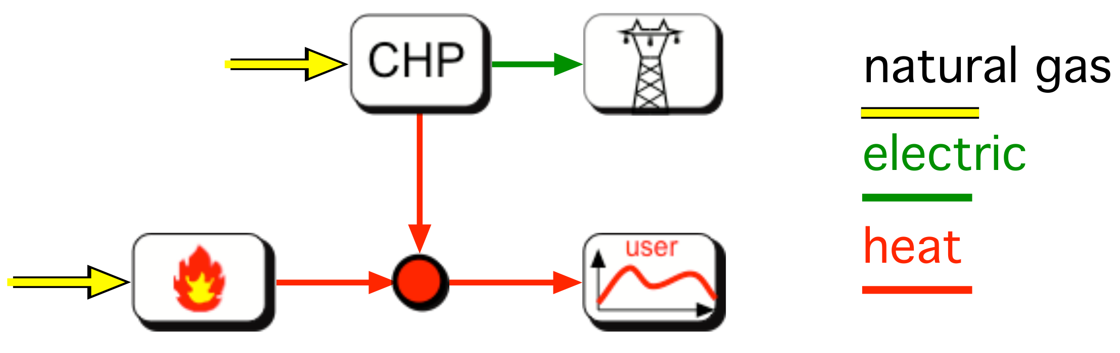
One of the simplest cases to describe this issue is represented in Figure 1. A cogeneration plant can provide heat to an end-user in at least two different ways: by burning a primary fuel in a boiler or by using the same fuel to supply a cogenerator that produces, at the same time, heat and electricity. This last form of energy can be sold to the grid, creating both a better exploitation of fuel and a form of economical revenue. The choice between these two modes of operation is related mainly to the selling price of electricity. As this price varies during the day, the operational mode changes and, for instance, makes it more convenient to run the cogenerator in hours when the electricity price is high while running the boiler at low price times. The Unit Commitment (UC) problem is then the definition of a strategy for finding the minimum running cost of the plant defining, at each time interval within a scheduling period, the on/off state of each machine and its production level.

This problem can be approached in different ways by means of mathematical programming and is solved here with an approach similar to that presented in [25].

The management cost C to be minimized is defined, in the present Italian case, as follows:

$$C=\sum _{j=1}^{N_{\mathrm{int}}}{c}_{NG}^{\left(nd\right)}{\displaystyle \frac{B_{\mathrm{t}}\left(t_j\right)}{{\eta }_{\mathrm{b}}{H}_{\mathrm{i}}}}\Delta t+c_{NG}^{\left(d\right)}{\displaystyle \frac{P_{\mathrm{t}}\left(t_j\right)}{{\eta }_{\mathrm{t}}{H}_{\mathrm{i}}}}\Delta t-c_{\mathrm{s}}\left(t_j\right)P_{\mathrm{e}}\left(t_j\right)\Delta t$$

(10)

where $c_{NG}^{\left(d\right)}$ and $c_{NG}^{\left(nd\right)}$ are the cost of natural gas without and with taxation due to different Italian fiscal regimes of the cogenerator and boiler, respectively; ${\eta }_{\mathrm{t}}$ and ${\eta }_{\mathrm{b}}$ are the thermal efficiencies of the cogenerator and boiler, respectively; $H_{\mathrm{i}}$ is the lower heating value of the natural gas; $B_{\mathrm{t}}\left(t_j\right)$ is the value of heating power of the boiler in the j-th interval; $P_{\mathrm{t}}\left(t_j\right)$ is the value of the thermal power of the cogenerator in the j-th interval; $P_{\mathrm{e}}\left(t_j\right)$ is the value of electrical power of the cogenerator in the j-th interval; $c_{\mathrm{s}}\left(t_j\right)$ is the unit selling price of electrical power to the grid at the j-th interval expressed in €/MWh; and $N_{\mathrm{int}}$ are the intervals with equal length for discretizing the scheduling period.

Although the efficiency of both the cogenerator and boiler varies at partial load conditions (as shown in [25]), in this work we focus our attention on other uncertain parameters with a higher influence on the running cost. Therefore, a simple model with constant efficiencies is used. Moreover, as will be shown later, the cogenerator often works at full power.

Equation (10) highlights that the management or operational cost for the plant is formed by the cost of burning fuel in the boiler and the cogenerator, reduced by the income owing to the electricity produced by the cogenerator and sold to the grid. It can be noticed that the objective function in Equation (10) also represents an economic balance influencing the dispatching of the two heat sources at each time interval. First, the unit with cheaper running cost is scheduled. Afterward, if the source capacity is lower than the heat demand, the unit with more expensive running cost contributes to covering the residual demand. Clearly Equation (10) is also subjected to energy balance constraints stating that heat production from the boiler and the cogenerator supply local demand $U_{\mathrm{t}}$, as well as that electricity is sold to the grid when produced by the cogenerator.

To evaluate the minimum cost C defined above, some data about the plant must be known. First, the cost of the fuel that will be burned inside components should be known. In the case of natural gas, a unit cost expressed, for instance, in €/smc is needed. In the same way, the thermal power demanded by the end-user has to be provided. This value is not scalar but rather an array of values defined for instance on a 24 h scheduling period. In Figure 2 the pattern of this end-user request related to a district heating in the winter season is shown.

Another array of data is the selling price of electricity. The price depends on the time of day and on the season. In Figure 3, an example of price dynamics taken from the Italian market is shown.

An example of commitment of the plant is shown in Figure 4: the power produced by the cogenerator is shown in blue and that of the boiler is shown in orange. These results are completely defined by the optimizer on the base of the minimum running cost. With the parameters considered it is observed that during daytime it is convenient to exploit as much as possible the energy coming from the cogenerator. In fact, the cogenerator is run during the central hours of the day when the electricity price is higher, while the boiler is used to produce the heat demand during the night and to cover peaks of request for which the cogenerator alone is not sufficient.

4. Sensitivity Analysis

The problem formulation proposed in the previous section gives the minimal running cost of the plant for a given price of natural gas, thermal load and selling price of electricity profiles. As was mentioned in the introduction, these values are often affected by errors and imprecisions, and how these uncertainties impact the minimal cost can be estimated by SA based on the approach proposed in Section 2. To this aim, the minimal running cost described in Equation (10) becomes, in the SA procedure, Equation (4). It is worth stressing that the cost evaluation proposed in Equation (10) is based on an optimization run, and that its computational burden is not negligible, thus preventing the use of an MC technique for evaluation of the variance of the cost. At any rate, in this case, an MC run is used as reference for the evaluation of the variance and for a comparison of the number of cost evaluation function calls required.

For the study proposed here, as already mentioned, the price of natural gas, the profiles of the thermal load and the selling price of electricity are considered as sources of uncertainty. For this purpose, three scalar and unitless quantities $p_1$, $p_2$ and $p_3$ are introduced as multiplicative factors. With reference to Equation (10):

• The cost of natural gas is multiplied by $p_1$;
• The heating load is multiplied by $p_2$;
• The selling price of electricity is multiplied by $p_3$.

The uncertainty is introduced by tuning the variation of the parameters $p_1$, $p_2$ and $p_3$. In this paper we consider both uniform and normal distribution. In the first case we consider a uniform distribution in the range (0.9, 1.1) to simulate a ±10% variation with respect to their nominal value. In the second case we consider a normal distribution having a mean of $\mu =1$ and standard deviation of $\sigma =0.05$. This choice makes it possible to simulate a variation of which 95% of the samples fall within the same range considered for the uniform distribution.

As explained earlier, in both cases the cost function of Equation (10) is taken as the $y\left(\mathbf{p}\right)$ function of Equation (4) and is used for the evaluation of the PCE coefficients defined in Equation (7).

By applying the procedure to the cogeneration case, the values of mean and of standard deviation of the cost can be plotted with respect to the number of function calls. This number corresponds in the MC method to the number of sampling trials, while in PCE it is the number of quadrature points that have to be used in the evaluation of the integral appearing in the numerator of Equation (7). The larger the number of points, the more accurate the evaluation of the PCE coefficients.

For both uniform (Figure 5) and normal variations (Figure 6) of the uncertain parameters, the PCE and MC techniques give similar results, but PCE is able to provide stable and convergent mean and standard deviation values after ten thousand cost function evaluations while MC is still far from convergence after 5 million calls.

PCE also allows the evaluation of sensitivity or Sobol’s indices. These values are evaluated in terms of both uniform and normal variation of input parameters. As explained above, both cases are set to analyze the variation of the parameters in the same range; therefore it is not strange to observe similar values for Sobol’s indices, as shown in

Table 1. Sobol’s indices in the case of uniform and normal distributions.

Variation	${\mathit{S}}_1$	${\mathit{S}}_2$	${\mathit{S}}_3$	${\mathit{S}}_{12}$	${\mathit{S}}_{13}$	${\mathit{S}}_{23}$	${\mathit{S}}_{123}$
Uniform	0.4931	0.1172	0.3891	0.0002	0.0002	0.0002	0.0000
Normal	0.4933	0.1177	0.3885	0.0002	0.0002	0.0001	0.0000

.

Some considerations can be drawn from the analysis of Table 1, in particular:

• The cost function is mostly affected by the natural gas cost as the sensitivity function $S_1$ reaches about 49% of the global variance in the case of both uniform and normal distributions;
• In terms of importance, the second parameter affecting the variance is the electricity price, whose influence $S_3$ is about 39% of the total variance;
• A lower importance parameter is the thermal load, whose effect $S_2$ is around 12%;
• Cross effects due to interaction of the parameters are not meaningful ($S_{12}$, $S_{13}$, $S_{23}$ and $S_{123}$ are negligible).

5. Discussion

The application of the PCE procedure to the cogeneration test case showed its effectiveness for the assessment of the propagation of uncertainties in the evaluation of operating cost minimization. Its computational cost is some orders of magnitude lower than an MC run and can thus be acceptable for the evaluation of KPI in complex energy systems whose simulation is computationaly intensive.

The main features of PCE also enable the analysis of the coupling between different causes of uncertainty, giving a deeper insight on the system.

In addition to mean and variance values, PCE creates a more accurate estimate of the parameters that mostly affect the output function by computing the sensitivity or Sobol’s indices. As a consequence, attention can be focused on these parameters, trying to reduce their uncertainty for getting more precise assessments of the cost function.