Python TensorFlow Big Data Analysis for the Security of Korean Nuclear Power Plants

Abstract

The Republic of Korea also suffered direct and indirect damages from the Fukushima nuclear accident in Japan and realized the significance of security due to the cyber-threat to the Republic of Korea Hydro and Nuclear Power Co., Ltd. With such matters in mind, this study sought to suggest a measure for improving security in the nuclear power plant. Based on overseas cyber-attack cases and attacking scenario on the control facility of the nuclear power plant, the study designed and proposed a nuclear power plant control network traffic analysis system that satisfies the security requirements and in-depth defense strategy. To enhance the security of the nuclear power plant, the study collected data such as internet provided to the control facilities, network traffic of intranet, and security equipment events and compared and verified them with machine learning analysis. After measuring the accuracy and time, the study proposed the most suitable analysis algorithm for the power plant in order to realize power plant security that facilitates real-time detection and response in the event of a cyber-attack. In this paper, we learned how to apply data for multiple servers and apply various security information as data in the security application using logs, and match with regard to application of character data such as file names. We improved by applying gender, and we converted to continuous data by resetting based on the risk of non-continuous data, and two optimization algorithms were applied to solve the problem of overfitting. Therefore, we think that there will be a contribution in the connection experiment of the data decision part and the optimization algorithm to learn the security data.

1. Introduction

Recently, there has been speculation in the Republic of Korea on the permanent shutdown of Shin-Gori Korean Nuclear Power Plant Units 5 and 6. The Korean government organized a speculation committee with the participation of citizens and announced the final recommendation. As a result, the restart of construction of nuclear power plant was recommended. The background of the initial speculation was to reflect the concern of the people regarding the safety of nuclear power.

In line with the severity of radiation leak of nuclear power plants, a decision was made with regard to denuclear awareness. Additional opinions in the speculation survey suggest the increasing need for the supplementation of safety. As such, the safety of a nuclear power plant is a serious national concern [1,2].

Among information system hackings for the last couple of years worldwide, a mobile service-based cyber-attack that poses a national risk is cyber-terrorism on an infrastructure facility such as nuclear power plant. A representative example is an attack on Iranian nuclear facility Stuxnet and the cyber-threat to the Republic of Korea Hydro and Nuclear Power Co., Ltd. The former showed that a nuclear power plant could be shut down by a direct cyber-attack, and the latter demonstrated that a cyber-hacking attack on a nuclear power plant could grip all the people in the country in terror. After these events, security has been reinforced as the risk of cyber-attack against the nuclear power plant was acknowledged [3,4].

The estimated damage by cyber-attack in national infrastructure facilities is far greater in size that it can have a nationwide effect and affect society overall. In particular, in the case of a nuclear power plant, it can inflict huge damage such as power outage and radiation leak, causing huge social chaos and continual damages. Reinforcing cyber-security against such threats requires analyzing the weaknesses of the control system periodically and strengthening the post-security measure check. The Cyber Security Plan (CSP) has been implemented as a measure for identifying digital equipment in the power plant control network and evaluating the risk level.

Nonetheless, there is a lack of operating and technical measures for maintaining the integrity of the control facility after identifying the digital equipment and checking weaknesses in the nuclear power plant control facility. Although compulsory digital equipment identification, weakness check, and media control are in place, there is a need to develop real-time detection measures against the newest malicious codes introduced to the control facility of power plants.

Accordingly, the study collected big data such as Internet provided to the control facilities, network traffic of intranet, and security equipment events and compared and verified them with machine learning analysis. After measuring the accuracy and time, the study proposed the most suitable analysis algorithm for the power plant in order to realize power plant security that facilitates real-time detection and response in the event of a cyber-attack. In Section 2, we show the related works. In Section 3, we describe the used data set, design, and the results of an experiment on the log data set. Finally, we conclude our study in Section 4.

2. Related Work

A multicore platform established on a large-scale computing cluster has led to promising development in the field of intelligent big data analysis recently, but processing an overwhelming volume of complex and delicate data generated by corporate or public IT centers and institutions is never enough [5]. During the period 2016~2017, MIT Media Lab Professor Dev Roy and his team engaged in research with six fact-checking organizations including PolitiFact and factcheck.org and checked 126,000 news articles that had been classified as true or fake news, concluding that the latter tended to spread faster and wider. His research work was published in the journal Science [6]. For this research, an AI was used to collect the activity data of three million readers who had read and shared such news for the analysis of the rate of news dissemination and number of shares on the network. As a result, the fake news was shared more broadly (70% pt.) than the true news and at much higher speed. This suggests that fake news spread much more widely than real news.

The professor’s research team reported that the analysis result from the physical statistics gathered for the comments attached to the news also supported the conclusion that sensational news can be spread rapidly regardless of whether it is true or not, adding, “Fake news with new and exciting features can be easily transmitted on the Internet and SNS” [6]. These big data analysis results can be visualized by using each fragment of the collected unstructured data as a piece of a jigsaw puzzle that would eventually reveal the whole picture once every one of them has been matched [5,6].

As for Big Data analysis, a regression method is generally used using variance. In case of log analysis, however, it is difficult to determine related variables, possibly caused by not following the Gaussian distribution [7,8,9]. Still, the criteria for determining the similarity and dissimilarity of character strings cannot be grounds for determining whether it is an invasion log or not. In particular, as for log related to invasion events, if the intention of the invaders is found, most of them are used to select other methods [10,11,12].

Nonetheless, this study assumed that the analysis using payload would detect whether the important asset route is overlapped or if a similar type of invasion is made. In particular, in the case of periodic log such as Spoofing, it seems analyzable by learning similar types. As for the analysis data, learning was carried out based on data relevant to invasion events. In addition, the study suggested a stable algorithm for the detection accuracy of invasion events and on overshooting and the small learning rate that often take place in learning [13,14,15,16,17]. Python is an advanced programming language released in 1991 by programmer Guido van Rossum. As an independent platform, interpreter-type, object-oriented, and dynamically typing interactive language [18,19,20,21,22], it can be used in various platforms, and it has a rich library (module). It is widely used in universities, various educational institutions, research institutions, and industries as an open source. In particular, the rich library related to big data analysis is a great help in big data analysis, machine learning, and graphic and academic research. The development version used in this study was Python 3 Version 3.6.1 [23].

Meanwhile, Chakraborty’s study [24] consider the case of defending enterprises that have been successfully hacked by imposing additional a posteriori costs on the attacker. Mercorio’s study [25] proposes a framework, namely discovery information using community detection (DICO), for identifying overlapped communities of authors from Big Scholarly Data by modeling authors’ interactions through a novel graph-based data model combining jointly document metadata with semantic information.

As an open source software library for machine learning used in Google products, TensorFlow was created by the Google Brain Team for research and product development. It was released as Apache 2.0 open source license on 9 November 2015. The programming languages are Python and C++, and it can be run not only on mobile environments like Android and iOS but also on 64-bit Linux, MacOS desktop, and multiple CPUs and GPUs in server systems.

The TensorFlow operation adopts the data flow graph method. The data flow graph is expressed as a direction graph expressing a mathematical calculation and the data flow using Node and Edge. Here, the node carries out operations such as mathematical calculation, data input/output, and data reading/storing. Edge represents the input/output relationship of data between nodes. The version used in this study is a graphic tool of Python TensorFlow Version 1.1.0 and Python TensorBoard [26].

Meanwhile, in the AlphaGo [27], they used to input features that was 11th to each pixel, as in the following (

Table 1. Input features for neural networks in AlphaGo.

Feature	# of Planes	Description
Stone color	3	Player stone/opponent stone/empty
Ones	1	A constant plane filled with 1
Turns since	8	How may turns since a move was played
Liberties	8	Number of liberties (empty adjacent points)
Capture size	8	How many opponent stones would be captured
Self-atari size	8	How many of own stones would be captured
Liberties after move	8	Number of liberties after this move is played
Ladder capture	1	Whether a move at this point is a successful ladder capture
Ladder escape	1	Whether a move at this point is a successful ladder escape
Sensibleness	1	Whether a move is legal and does not fill its own eyes
Zeros	1	A constant plane filled with 0
Player color	1	Whether current player is black

).

That means they used 19 × 19 × 48 because it has 48 dimensions and 19 pixels × 19 pixels. We might be thinking about using this method if we had so many features in the analysis data.

3. Python TensorFlow Big Data Analysis for the Security of Korean Nuclear Power Plants

The big data analyzed in this study were collected from 00:02, 28 July 2017 to 23:30, 1 September 2017. The dataset was composed of the Republic of Korea Hydro Nuclear APT equipment log, virus vaccine equipment log, IPS log, output security device log, and DRM log. It consists of “Time”, “Equipment Name”, “Operation Status”, and “Payload”. A big data analysis was carried out using Python. The learning data were 5638 lines including 274 leaked data. A total of 2000 data were used as learning data including 96 leaked data. The remaining 3638 data were measured as verification targets.

The function formula is y = Wx + b, and it applies a 2000 × 2 matrix using 2 labels and 2000 learning data in y and a 2000 × 696 matrix using a vector with learning data of 2000 dimensional vectors and 696 data in x. The W value was then estimated, and whether the 178 information-leaked data belonging to 3638 could be accurately found was reviewed using the W value and 3638 lines and labels used in the test. This study compared the algorithm that minimizes cross entropy.

Figure 1 shows the numbers converted into a decimal, and they had no meaning. It is important in the order and overlap in the character string analysis. Despite the difficulty in confirming the usage interval using some other characters, it showed the tendency of redundancy of some characters. There are many direct connections in the data order in the figure as well as many data redundancies.

3.1. Define Data Features

Since considering data learning, we needed to define the characteristics of the data.

Table 2. Example of log dataset: in the log of ExploitMalware, some charaters is Korean, that means are “메인홈페이지”: main site in the homepage, “중간”: middle, “탐지”:detection and “에러페이지 클로킹”: cloaked error page.

Log	Contents
Log of common information	WRK_IDX: “xxxxxx” SERVER_FLAG: “0” USBSERIAL: “AAFxxxxxxxx” MNUM: “xxxxxxxxxx-0108” USER_ID: “xxxxxxxx” IP_ADDR: “xxx.xxx.xxx.xxx” ONOFF_FLAG: “xx” WRKLOG_FILENAME: “xxxxxxxx_setup.exe” WRKLOG_SRC: “C:\Users\User\Desktop” WRKLOG_DST: “USB” WRKLOG_TYPE: “2” LOG_DT: “2017-09-17 03:24:01.0” WORK_DT: “2017-09-17 18:12:43.0” GROUP_CD: “xxxxxxxx” DEL_FLAG: “x” WORK_IP: “xxx.xxx.xxx.xxx” WORK_USER_NM: “null” WORK_GROUP_CD: “null” WORK_GROUP_NM: “null” WORK_SERVER_IP: “xxx.xxx.xxx.xxx” WORK_SERVER_NM: “nProtect Solution” USB_CMT: ““
Log of information leakage	WRK_IDX: “xxxxxx” SERVER_FLAG: “1” USBSERIAL: “AAFxxxxxxxx” MNUM: “xxxxxxxxxxxx-0001” USER_ID: “xxxxxxx” IP_ADDR: “xxx.xxx.xxx.xxx” ONOFF_FLAG: “xx” WRKLOG_FILENAME: “signCert.der” WRKLOG_SRC: “USB” WRKLOG_DST: “USB” WRKLOG_TYPE: “x” LOG_DT: “2017-09-19 09:19:04.0” WORK_DT: “2017-09-19 09:19:06.0” GROUP_CD: “xxxxxxxx” USB_CMT: ““ DEL_FLAG: “x” WORK_IP: “xxx.xxx.xxx.xxx” WORK_USER_NM: “null” WORK_GROUP_CD: “null” WORK_GROUP_NM: “null” WORK_SERVER_IP: “xxx.xxx.xxx.xxx” WORK_SERVER_NM: “nProtect Solution”
Log of Sniper	[SNIPER-1821] [Attack_Name=(xxxxx)TCP DRDOS Attack], [Time=2017/09/13 09:03:38], [Hacker=xxx.xxx.xxx.xxx], [Victim=xxx.xxx.xxx.xxx], [Protocol=tcp/xxxxx], [Risk=xxx], [Handling=xxx], [Information=], [SrcPort=xxx], [HackType=xxxxx]
Log of Exploit-Malware	DETECT|WAF|2017-09-12 09:36:57|10.221.0.97|v4|xxx.xxx.xxx.xxx|xxxxxx|xxx.xxx.xxx.xxx|xxxx|메인홈페이지|Error Page Cloaking_404|중간|탐지|xxx|에러페이지 클로킹|status code 404|http|www.xxx.xx.xx|478|GET/gate/js/write.js HTTP/1.1 Accept: application/javascript, */*;q=0.8 Referer: http://www.xxx.xx.xx/gate/xxxxxxxx.do Accept-Language: ko-KR User-Agent: Mozilla/5.0 Accept-Encoding: xxxx, deflate Host: www.xxxx.xx.xx DNT: xxx Connection: Keep-Alive Cookie: WCN_KHNPHOME=xxxxxxxxxxxxxxxxxxxx WCN_GATE=xxxxxxxxxxxxxxxxx

is related to this. In the existing Alphago, it was 19 × 19 × 48, but we applied the server instead of the pixel and insert log values classified as information leakage, printout security, ExploitMalware, Local Worm Detected, SniperIPS, and Virusspware. Therefore, if there are 6 servers, it becomes 1 × 6, and additionally, the characteristics corresponding to each log are inserted as shown in Table 2: it was masked to IP, FLAG, etc.

In the case of the IP in the learning data, the numbers from 0 to 255 were divided into four, and in the case of FLAG, a separate index was implemented based on the risk. Additionally, in the case of Char, such as a file name, it was converted and applied based on consistency. Here, if the file name that can be considered as an important file is “signCert.der”, the total number of characters is 12 including “.”. Therefore, in the case of “signCert.xxx”, the value of consistency was 8/12. If the file name is “sign.der”, the denominator does not change, so the value was 8/12. That is, because we have the names of critical files.

Therefore, as shown in

Table 3. Applied features data.

Feature	# of Planes	Description
Information leakage	23	Value of each item without a date (more detail is included in the patent, which has been excluded)
Printout security	23
ExploitMalware	10
Local Worm Detected	10
SniperIPS	10
Virusspware	5
Total	81

, the singular value for each server was set based on the characteristic value.

3.2. Data Learning

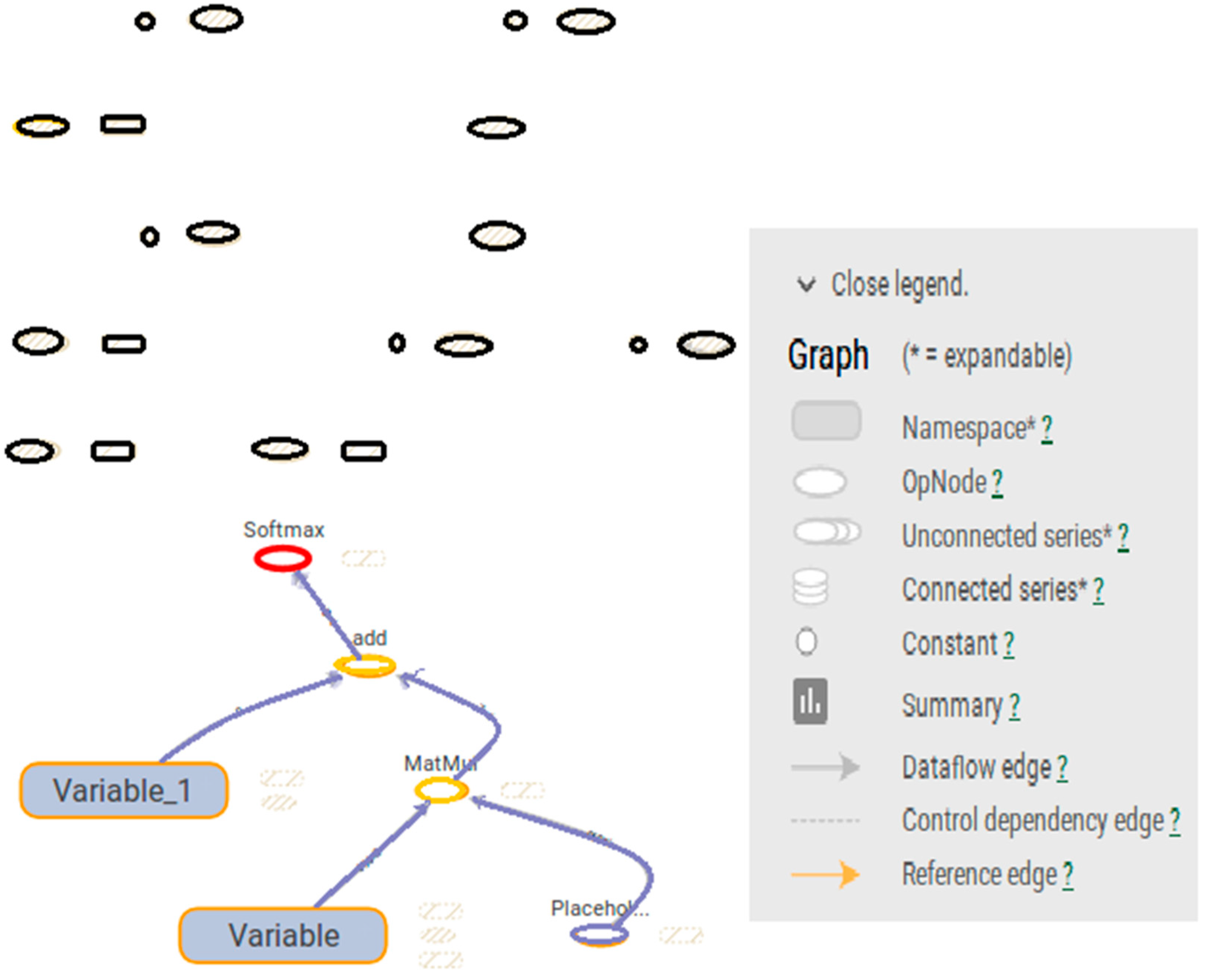
Figure 2 is a visualized graph of the calculation graph in TensorBoard, a function of TensorFlow that visualizes the calculated graph and related values.

Unlike other machine learning frameworks, it is embedded, and it provides a graph format. It shows how the data in the computed graph change as the data flows over the graph. Figure 2 depicts the composite multiplication of the values of two variables, X and Y.

It means that the basic function expression of the experiment above is y = ax + b. Variable means a value; Variable 1 refers to the b value, yellow Placeholder indicates the input x value, and final Softmax is an estimated Y value provided from TensorFlow. In an existing neural network, the Sigmoid function was used. Softmax of TensorFlow estimated the Y value according to a probability value based on Sigmoid.

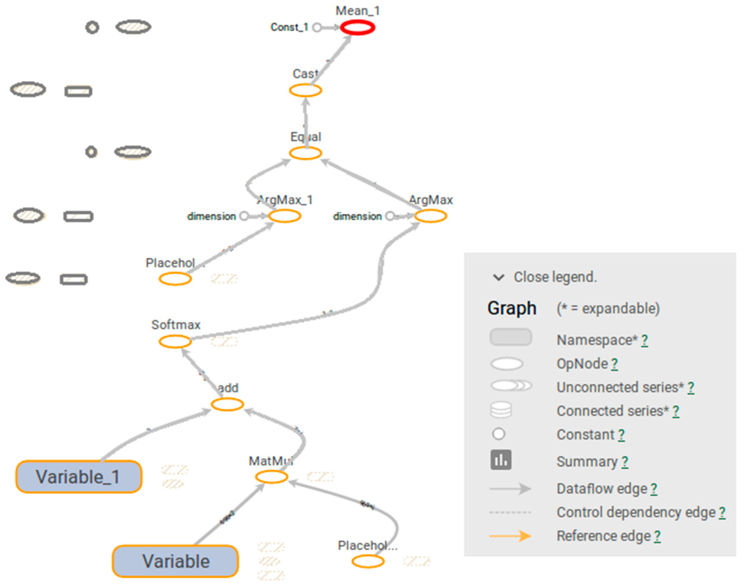
Figure 3 shows the structure for measuring accuracy by comparing the validation data y_ after learning with the value of y calculated by learning, where ArgMax_1 is the y_ value, i.e., the prior result value. The final two values were compared, and accuracy was measured as an average. Here, the input value was a structure for sequentially inputting many values applying the matrix structure as it stands.

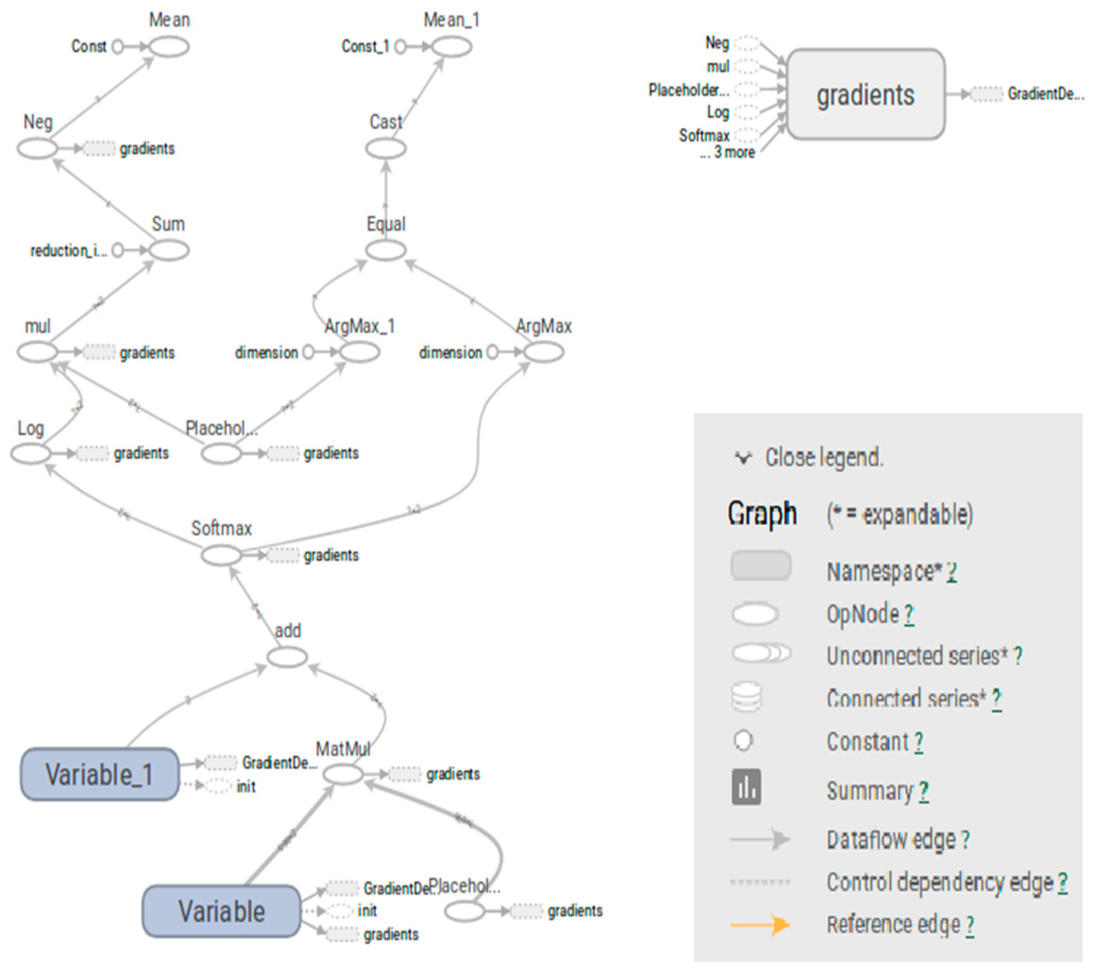
Figure 4 shows the structure for obtaining the minimum value of entropy using Softmax, which calculated the output value with probability instead of applying it to Sigmoid. Gradient Descent (G-Descent) means the gradient descent method.

The general gradient method can determine the minimum value through the derivative of the estimated curve. The method used here was a gradient descent method that limits the travel distance by using the value of the learning rate. This is because the algorithm that prevents a return is mainly used, and it neither makes a big jump nor goes beyond a local trough. The estimate was determined by the minimum mean sum of such learning.

Figure 5 presents the entire flow at once and shows the accuracy based on storage with the estimate and input Y_ value. Thus, it was designed with the two structures above.

Figure 5 and Figure 6 had the same structure, with the minimization algorithm as the only difference. While Adam is known to be a quick time algorithm, the G-Descent algorithm is known to be highly accurate. Thus, the study measured the results by inputting actual big data.

Figure 7 shows the structure of the convolutional neural network (CNN). Unlike the existing single network, three hidden layers were added. From the top left, the first hidden layer was further arranged with 32 of 5 × 5 using 5 × 5 × 1 × 32. In the second one, the first node was divided with 5 × 5 × 32 × 64. The third one was a fully connected layer with 7 × 7 × 64 × 1024.

The first hidden layer in Figure 8 was generated by decomposing a total of 32 small figures of 5 × 5 from the 28 × 28 picture as shown in the second figure.

It means the generation of a node. Compound multiplying was done to enhance the accuracy of probability by cutting some parts additionally. It means to divide [1,2,3,4] by [1,2], [3,4], where the first extension is a 5 × 5 size and 28 pixels are moved to the left by 1 column to make 24.

In this study, dropout was established for multiple node calculation and deletion of unnecessary nodes, but all connections were used by setting 1.0 mainly to avoid overfitting.

3.3. Analysis of Experiment Results and Performance Evaluation

Evaluation in general machine learning is directly related to overshooting and a small learning rate problem, accuracy, and time depending on how the learning rate is adjusted during learning. In the first place, when the G-Descent algorithm is used, a problem occurs wherein the user determines the learning situation.

Overshooting refers to a phenomenon wherein the value of W is minimized, subsequently going beyond the lowest point and proceeding to the relative value and going to infinity. Figure 9 shows that overshooting occurred even in learning less than 10 times when the learning rate was set to 0.015. Overshooting occurred up to 0.00015. In this experiment, the learning rate was set to 0.000015 for stable progress, but learning took longer.

Figure 10 shows a problem wherein the learning rate was set to 0.0000015. Despite the 1000 times of learning, it failed to reach the lowest point due to the short progress distance and ended with 99.17%.

Figure 11 shows that there was no big difference in overall accuracy, but there was about 50% time difference for the same 1000 times of learning. The current TensorFlow was based on CPU, which took more time. In the case of CNN, both accuracy and time decreased. Since it calculated all output values of the multilayer network, the time increase was huge, but accuracy depended on the reflection of connection of all layers. When the layer connection increased, accuracy increased, but time decreased.

Figure 12 and Figure 13 show the learning in 5 divided data with 201 events, 1151 events, 1000 events, 76 events, and 26 events classified into Fireeye_EX Hangul, Multiple Exploit Malware Types, Possible Local Worm Detected, and sniperIPS_low_Log, respectively. Out of the 110,000 cases classified as Possible Local Worm Detected, 15,000 events were tested. As a result, it took some time, but the accuracy was high. This means that 13 cases were determined as different events out of 15,000 cases, calculated as (1 − 0.999133) × 15,000 = 13. By learning the other invasion factors with noise, the actual data analysis can be more accurate.

In Figure 14, accuracy and time were measured by applying the Adam algorithm used in the calculation of the minimum value supported by TensorFlow and the commonly used G-Descent in learning a single class. In addition, it explained the accuracy and time in the case of learning by adding four additional noise classes to single class detection.

Meanwhile,

Table 4. Experiments with three algorithms of machine learning.

No.	Order	Algorithm	Learning Method	Accuracy	Time (/s)	Comparison Result
1	1st	Adam algorithm	Single learning	0.9989	15.86	Faster than G-Descent (16.83)
2		G-Descent algorithm		0.9989	32.69	Accuracy is the same as that of Adam
3		CNN algorithm		0.9510	370.06	Exceeded time
1	2nd	Adam algorithm	Noise insertion	0.9991	44.62	Faster than G-Descent (0.68)
2		G-Descent algorithm		0.9994	45.30	Accuracy is higher than Adam (0.0003)

presents the result of the experiment with three algorithms of machine learning. In the 1st experiment, the Adam algorithm analysis was the fastest with 15.86 /s, and accuracy was the same. The CNN algorithm showed far lower performance in terms of time or accuracy.

In the first experiment, the accuracy was the same. Thus, in the second experiment, when learning was done by inserting noise, the accuracy of the G-Descent algorithm was excellent. In other words, G-Descent was excellent in terms of accuracy, and Adam was excellent in terms of time. Learning with noise insertion can lead to more accurate results in actual data analysis. The time measurement result was 0.68 /s, and the Adam algorithm was excellent. Accuracy was not different in single learning, and G-Descent was 0.0003 as a result of noise learning. Moreover, G-Descent is inconvenient as it needs additional settings such as the learning rate.

As a result of the comparison between two machine learning algorithms, Adam was more advantageous than G-Descent as the algorithm of the big data analysis of a nuclear power plant.

Then, the question of whether an algorithm with quick analysis speed is suitable for the log analysis of power plant arises. If the result of the comparison analysis of accuracy and analysis speed is selected, the power plant cannot give up one of the two because, as mentioned in the introduction, damages caused by cyber-attacks on critical infrastructure of the country can mean a national disaster.

Table 5. Test result comparison with three algorithms of machine learning.

No.	Order of Experiment Scenario	Learning Count	Remarks
1	G-Descent algorithm ⇒ Adam algorithm	500:500	Single learning
2	Adam algorithm ⇒ G-Descent algorithm	500:500
3	G-Descent algorithm ⇒ Adam algorithm	500:500	Noise Insertion
4	Adam algorithm ⇒ G-Descent algorithm	500:500

shows the test result comparison with three algorithms of machine learning. Based on the results of the previous experiments, two models were created. Experiments were conducted using four methods. To acquire accuracy and analysis speed, two algorithms were combined. To obtain the optimal algorithm, it was divided into two. First, it carried out a method of increasing speed with the Adam algorithm after increasing accuracy with the prerequisite learning of the G-Descent algorithm (G-Descent ⇒ Adam). Second, it carried out a method of increasing accuracy with the G-Descent algorithm after increasing speed with the Adam algorithm (Adam ⇒ G-Descent). Both methods were experimented on for 500 times each.

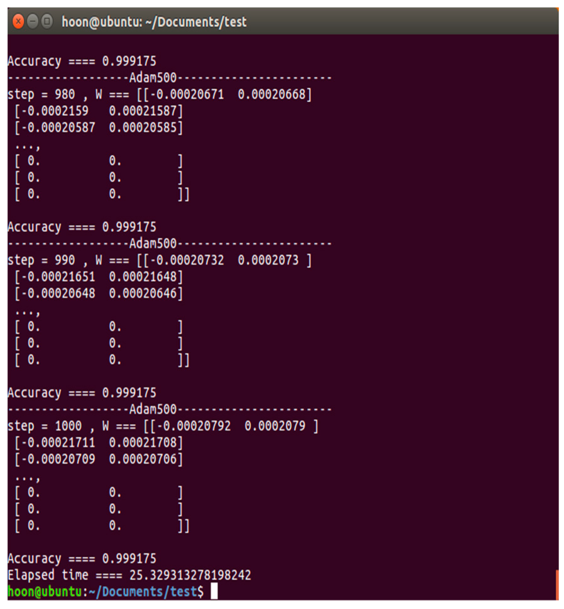
Figure 15 is the result of the scenario 1 experiment. Specifically, it is a result of single learning (500 times) of the Adam algorithm after the learning of the G-Descent algorithm (500 times). As a result of a total of 1000 times of learning, accuracy was 0.999175, and measurement time was 25.32931 /s.

Figure 16 is the result of the scenario 2 experiment. Specifically, it is a result of single learning (500 times) of the G-Descent algorithm after the learning of the Adam algorithm (500 times). As a result of a total of 1000 times of learning, accuracy was 0.998351, and measurement time was 14.46075 /s.

Figure 17 is the result of the scenario 3 experiment. Specifically, it is a result of noise insertion into the Adam algorithm after the learning of the G-Descent algorithm for 500 times. As a result of a total of 1000 times of learning, accuracy was 0.999133, and measurement time was 44.93227 /s.

Figure 18 is the result of the scenario 4 experiment. Specifically, it is a result of noise insertion into the G-Descent algorithm after the learning of the Adam algorithm for 500 times. As a result of a total of 1000 times of learning, accuracy was 0.999133, and measurement time was 49.86963 /s.

Figure 19 is a visualization graph provided by TensorBoard, which is a visualization tool of TensorFlow. As TensorFlow teaches the neural network, it shows the process of optimization and graphs the indicators. The vertical means the number of machine learning times, with the horizontal line as the values of weight. This corresponds to a when y = ax + b, and If you do not include the noise value in the experiment, the slopes can be divided into two higher distributions. A and B in Figure 17 mean that 1,000 times of learning were done in G-Descent ⇒ Adam order, and that 1000 times of execution were each carried out. The top two lines and the two bottom lines indicate that the weights distribution value depended on which one was first studied. Figure 19B on the top row shows the weight distribution that seems to have not been trained despite the 500:500 learning curve, while the bottom line D shows the evenly distributed slope. As a result, learning Adam first rather than G-Descent was found to be advantageous in class classification.

Figure 20 is a graph comparing the accuracy of single learning and noise insertion learning. The vertical line indicates accuracy, and the width indicates the learning unit. The vertical scale indicates the accuracy of a single cell with 100 times of learning, the blurred line denotes the accuracy when verifying with learning data, and the darker line indicates the accuracy with validation data after learning with learning data. The reason the diagonal line (dotted line) appeared is that the noise was caused by the phenomenon wherein accuracy suddenly dropped again while double learning was processed. Since it is a result of the experiment, it is expressed as is. The figure above is a curved graph with winding in case of single learning (Figure 20C,D), and the noise learning (Figure 20A,B) shows a curved graph without winding, showing more stability.

The currently experimented learning data covered 2000–3000 cases. The graph was not shown in detail. Experimenting with at least 100,000 cases may produce a more detailed graph.

Table 6. Final result table obtained from 4 scenarios.

No.	Scenario	Learning Method	Accuracy	Time (/s)	Result
1	Adam algorithm ⇒ G-Descent algorithm	Single learning	0.998351	14.46075	Faster than G-D ⇒ Adam (10.86856)
2	G-Descent algorithm ⇒ Adam algorithm		0.999175	25.32931	Accuracy is higher than Adam ⇒ G-D (0.000824)
3	Adam algorithm ⇒ G-Descent algorithm	Noise insertion	0.999133	49.86963	The two algorithms have the same accuracy
4	G-Descent algorithm ⇒ Adam algorithm		0.999133	44.9327	Faster than Adam ⇒ G-D (4.93693)

shows the final results by the four scenario methods. As for single learning, the method of enhancing accuracy with the G-Descent algorithm after enhancing speed with the Adam algorithm was faster at 10.86856 /s. Accuracy was higher when G-Descent was learnt first. The noise learning results show that G-Descent was faster with the same accuracy.

Meanwhile, Figure 21 compares the learning time from single learning and from noise insertion. Inserting noise can increase accuracy but learning takes longer. Although not mentioned in this experiment, when an experiment at a learning ratio of 900:100 was tested additionally, the speed of Adam ⇒ G-Descent was 15.0898 /s, and that of G-Descent ⇒ Adam was 15.4410 /s. Accuracy had differences in almost three decimal places.

As a result of the experiment, the G-Descent time of the single algorithm was 14.46075 /s, with Adam recording 25.3293 /s. When the problem of selecting either time or accuracy in a single algorithm was tested and measured in four types in a double manner, Adam ⇒ G-Descent recorded the same time with 14.46075 /s, which had no difference with single Adam but had increased accuracy.

The test result suggests that Adam ⇒ G-Descent was suitable as a recommended machine learning algorithm for the big data log analysis to enhance the security of the nuclear power plant.

4. Conclusions

This study designed and proposed a nuclear power plant control network traffic analysis system that satisfies the security requirements and in-depth defense strategy based on recent overseas cyber-attack cases and control facility attacking scenario against nuclear power plants.

To enhance the security of the nuclear power plant, the study collected big data such as the internet provided to the control facilities, network traffic of the intranet, and security equipment events and compared and verified them with the machine learning analysis. After measuring accuracy and time, the study proposed the most suitable analysis algorithm for the power plant through comparison and analysis. To find a suitable algorithm, the study compared and tested Adam, G-Descent, and CNN algorithm. In the 1st test result, in terms of the analysis study, the Adam algorithm was predominant, and G-Descent had the highest accuracy. CNN was excluded as it had more than double the speed difference compared with other algorithms. The suitable algorithm for the control network analysis requires not only accuracy but also analysis time. Real-time analysis on the attack against power plants needs to be short and quick but accuracy cannot be compromised.

As a result of the experiment, the Adam algorithm ⇒ G-Descent algorithm method recorded faster analysis speed with 10.86858 /s than the G-Descent algorithm ⇒ Adam algorithm. Likewise, there was no significant difference in accuracy. As the experiment environment was a result of learning using a workstation memory, the speed difference is expected to be greater if a graphic card is used.

In addition to the modified technique of the optimization technique, this study presents a method on how to apply the data for machine learning in relation to security, and at the same time, if it is not continuous data, converts it to continuous data using a specific index. By this, we tried to present a method of avoiding by using two optimization techniques in relation to the possibility of learning and the problem of overfitting, especially the problem of learning to use a character. In a future study, we will conduct research on Bagging (Bootstrap) in relation to the lack of data related to intrusion and hacking.

References

1. Sangil, P.; Jun-Ho, H. Effect of cooperation on manufacturing it project development and test bed for successful industry 4.0 project: Safety management for security. Processes 2018, 6, 1–31. [Google Scholar]
2. Diederik, P.K.; Jimmy, L.B. Adam: A method for stochastic optimization. In Proceedings of the 3rd International Conference for Learning Representations (ICLR’15), San Diego, CA, USA, 7 May 2015. [Google Scholar]
3. LeCun, Y.; Bengio, Y.; Hinton, G. Deep learning. Nature 2015, 521, 436–444. [Google Scholar] [CrossRef] [PubMed]
4. Sermanet, P.; Eigen, D.; Zhang, X.; Mathieu, M.; Fergus, R.; LeCun, Y. Overfeat: Integrated recognition, localization and detection using convolutional networks. In proceeding of 2nd International Conference on Learning Representations, Banff, AB, Canada, 14–16 April 2014. [Google Scholar]
5. Jun-Ho, H. Big data analysis for personalized health activities: Machine learning processing for automatic keyword extraction approach. Symmetry 2018, 10, 93. [Google Scholar]
6. Vosoughi, S.; Roy, D.; Aral, S. The spread of true and false news online. Science 2018, 359, 1146–1151. [Google Scholar] [CrossRef] [PubMed]
7. Lee, S.; Jun-Ho, H. An effective security measures for nuclear power plant using big data analysis approach. J. Supercomput. 2019, 75, 4267–4294. [Google Scholar] [CrossRef]
8. Birkenmeier, G.F.; Park, J.K.; Rizvi, S.T. Principally quasi-Baer ring hulls. In Advances in Ring Theory; Trends in Mathematics; Springer: Berlin/Heidelberg, Germany, 2010; pp. 47–61. [Google Scholar]
9. Lantz, B. Machine Learning with R; Packt Publishing Ltd.: Birmingham, UK, 2013. [Google Scholar]
10. Mnih, V. Playing Atari with Deep Reinforcement Learning. In Proceedings of the 2013 Conference on Neural Information Processing Systems (NIPS) Deep Learning Workshop, Lake Tahoe, CA, USA, 9 December 2013. [Google Scholar]
11. Murphy, K.P. Machine Learning: A Probabilistic Perspective; MIT Press: Cambridge, MA, USA, 2012. [Google Scholar]
12. Sagiroglu, S.; Duygu, S. Big data: A review. In Proceedings of the 2013 International Conference on Collaboration Technologies and Systems (CTS), San Diego, CA, USA, 20 May 2013; pp. 42–47. [Google Scholar]
13. Zhu, X.; Zhang, L.; Huang, Z. A sparse embedding and least variance encoding approach to hashing. IEEE Trans. Image Process. 2014, 23, 3737–3750. [Google Scholar] [CrossRef] [PubMed] [Green Version]
14. Zhu, X.; Zhang, S.; Jin, Z.; Zhang, Z.; Xu, Z. Missing value estimation for mixed-attribute data sets. IEEE Trans. Knowl. Data Eng. 2011, 23, 110–121. [Google Scholar] [CrossRef]
15. Zhang, S. KNN-CF Approach: Incorporating Certainty Factor to kNN Classification. IEEE Intell. Inform. Bull. 2010, 11, 24–33. [Google Scholar]
16. Lu, L.R.; Fa, H.Y. A density-based method for reducing the amount of training data in kNN text classification. J. Comput. Res. Dev. 2004, 4, 3. [Google Scholar]
17. Zhao, D.; Zou, W.; Sun, G. A fast image classification algorithm using support vector machine. In Proceedings of the 2nd International Conference on Computer Technology and Development (ICCTD) IEEE, Cairo, Egypt, 2 November 2010; pp. 385–388. [Google Scholar]
18. Wu, X.; Zhang, C.; Zhang, S. Database classification for multi-database mining. Inf. Syst. 2005, 30, 71–88. [Google Scholar] [CrossRef]
19. Wu, X.; Zhang, S. Synthesizing high-frequency rules from different data sources. IEEE Trans. Knowl. Data Eng. 2003, 15, 353–367. [Google Scholar]
20. Deng, Z.; Zhu, X.; Cheng, D.; Zong, M.; Zhang, S. Efficient kNN classification algorithm for big data. Neurocomputing 2016, 195, 143–148. [Google Scholar] [CrossRef]
21. Xu, Y.; Zhang, Y.; Zhao, J.; Yang, Z.; Pan, X. KNN-based maximum margin and minimum volume hyper-sphere machine for imbalanced data classification. Int. J. Mach. Learn. Cybern. 2019, 1, 357–368. [Google Scholar] [CrossRef]
22. Jordan, M.I.; Mitchell, T.M. Machine learning: Trends, perspectives, and prospects. Science 2015, 349, 255–260. [Google Scholar] [CrossRef] [PubMed]
23. Moscato, V.; Picariello, A.; Sperlí, G. Community detection based on game theory. Eng. Appl. Artif. Intell. 2019, 85, 773–782. [Google Scholar] [CrossRef]
24. Chakraborty, T.; Jajodia, S.; Katz, J.; Picariello, A.; Sperli, G.; Subrahmanian, V.S. FORGE: A Fake Online Repository Generation Engine for Cyber Deception. In IEEE Transactions on Dependable and Secure Computing; IEEE: Piscataway, NJ, USA, 2019. [Google Scholar]
25. Mercorio, F.; Mezzanzanica, M.; Moscato, V.; Picariello, A.; Sperli, G. Dico: A Graph-db Framework for Community Detection on Big Scholarly Data. In IEEE Transactions on Dependable and Secure Computing; IEEE: Piscataway, NJ, USA, 2019. [Google Scholar]
26. Sangdo, L. An Improved Big Data Analysis Technique for Enhanced Security of Nuclear Power Plant System. Ph.D. Thesis, School of Computer, Soongsil University, Seoul, Korea, 2018. [Google Scholar]
27. Silver, A.D.; Huang, C.J.; Maddison, A.; Guez, L.; Sifre, G.; Van Den, D.; Sander, D. Mastering the game of go with deep neural networks and tree search. Nature 2016, 529, 484–489. [Google Scholar] [CrossRef] [PubMed]
Figure 1. Example of converting the security log to the number of characters: the vertical axis is the number of words, the horizontal axis is the word dictionary; the word dictionary is created for words appearing in the current data.
Electronics 09 01467 g001
Figure 2. Visualized graph of the calculation graph in TensorBoard.
Electronics 09 01467 g002
Figure 3. Comparison structure for the validation data application and Y value.
Electronics 09 01467 g003
Figure 4. Learning and entropy minimization structure.
Electronics 09 01467 g004
Figure 5. Structure using Adam.
Electronics 09 01467 g005
Figure 6. Structure using G-Descent.
Electronics 09 01467 g006
Figure 7. Structure using the convolutional neural network.
Electronics 09 01467 g007
Figure 8. Diagram of the multilayer network structure.
Electronics 09 01467 g008
Figure 9. Data overshooting.
Electronics 09 01467 g009
Figure 10. Small learning rate.
Electronics 09 01467 g010
Figure 11. Accuracy and time using the convolutional neural network (CNN).
Electronics 09 01467 g011
Figure 12. Accuracy and time of G-Descent in 5 cases.
Electronics 09 01467 g012
Figure 13. Accuracy and time of Adam in 5 cases.
Electronics 09 01467 g013
Figure 14. Accuracy comparison graph.
Electronics 09 01467 g014
Figure 15. Scenario 1 experiment result: single learning (G-Descent ⇒ Adam).
Electronics 09 01467 g015
Figure 16. Scenario 2 experiment result: single learning (Adam ⇒ G-Descent).
Electronics 09 01467 g016
Figure 17. Scenario 3 experiment result: noise learning (G-Descent ⇒ Adam).
Electronics 09 01467 g017
Figure 18. Scenario 4 experiment result: noise learning (Adam ⇒ G-Descent).
Electronics 09 01467 g018
Figure 19. Visualization performance evaluation provided by TensorBoard: the vertical axis is the number of training, the horizontal axis is the number of weight; (A,C) is not include noise data, and (B,D) is include noise data; It is to see the result of how well the slope is distributed, and (B,D) in the figure bring an even distribution that is not biased in one place as the learning continues.
Electronics 09 01467 g019
Figure 20. Graph comparing the accuracy of single learning and noise insertion learning: the vertical axis is the accuracy, the horizontal axis is the number of training; It looks like not different between noise insertion learning and single learning but this graph shows combinational learning to (C) from (A) or to (A) from (C); (B,D) is more stable aspect the accuracy.
Electronics 09 01467 g020
Figure 21. Comparison of learning time from single learning and from noise insertion.
Electronics 09 01467 g021