A Fast Weakly-Coupled Double-Layer ESKF Attitude Estimation Algorithm and Application

Abstract

Aimed at the problem of small unmanned aerial vehicle (UAV) attitude solution accuracy and real-time performance in short-range navigation flight, in this paper, we propose a fast weakly-coupled double-layer error-state Kalman filter (DL-ESKF) attitude estimation algorithm. Considering the application of short-range navigation, we designed an improved attitude error model for low-cost gyroscope/accelerometer/magnetometer devices. In addition, we reasonably simplified certain factors that affect the attitude solution to reduce the filtering calculation burden. For the data coupling phenomenon caused by the different sampling frequencies of the attitude sensor data in the filtering process, we designed a new attitude algorithm combined with the ESKF and hierarchical filter. The first layer of filters used an accelerometer and the second layer used a magnetometer to correct the attitude error. We also built an offline and real-time test platform to verify the performance of the proposed algorithm in a simulation and flight test environment compared with the classic attitude algorithms. The experimental results demonstrated that the proposed algorithm not only improved the attitude solution accuracy and stability but also reduced the filter running time.

1. Introduction

In the autonomous navigation and control of small unmanned aerial vehicles (UAVs) [1], accurate and reliable attitude estimation [2,3] is indispensable. In recent years, the microelectromechanical systems inertial measurement unit (MEMS IMU) [4,5] has been developed rapidly. Due to the advantages [6,7] of being lightweight, small size, low power consumption, and low cost, the MEMS IMU has become an excellent selection for small UAVs in attitude estimation. The UAV attitude estimation system [8,9] is composed of a gyroscope, accelerometer, magnetometer, and microprocessor, and uses information fusion algorithms to estimate the optimal attitude vector, which includes the roll angle, pitch angle, and yaw angle. This can still output steady attitude information without the data from the other sensors.

There are two main fusion algorithms to fuse the attitude sensors data—constant gain observer (complementary filter) and Kalman filter. The complementary filter is a multisensor fusion algorithm that integrates the gyroscope angular rate, corrects the gyroscope bias [10], and then uses the accelerometer measurement value to correct the roll angle and pitch angle and the magnetometer measurement value to correct the yaw angle [11]. The state variable of the complementary filter can usually be defined in the form of an attitude vector, such as a Euler angle or quaternion and gyro bias [12].

The complementary filter is a pretty simple algorithm, and this has very little computation burden and is easy to implement in the application. These advantages make it more suitable for low-cost embedded systems. Euston M [13] proposed a complementary filter attitude algorithm, which combined low-cost IMU [14,15] and a magnetometer using the first-order dynamic model to provide good attitude estimation for the UAV. Wu J [16] proposed a fast complementary filter fusion algorithm based on quaternion attitude estimation and designed a step-by-step filter to eliminate the effect of magnetometer outliers to improve the solution accuracy and real-time performance.

Another attitude fusion algorithm is the Kalman filter [17,18] that can model and optimize the attitude sensors system to estimate the UAV attitude. The Kalman filter can be divided into two parts—time update and measurement update when performing attitude solutions [19]. The angular rate of the gyroscope is used to calculate the attitude prediction value at a faster data sample frequency in the time update section. The acceleration of the accelerometer and the magnetic field strength of the magnetometer correct the attitude prediction at a different data sample frequency in the measurement update section and, meanwhile, constantly adjust the attitude error [20] through the Kalman filter gain.

Song Y [21] proposed a quaternion attitude Kalman filter algorithm and used the adaptive filter to modify the measurement noise covariance matrix. This solved the problem of large errors of MEMS IMU [22,23] and reduced the impact of gyroscope random errors in attitude estimation. Sabatelli S [24] proposed a quaternion double-level Kalman filter of the attitude estimation with a 9-axis MEMS IMU. The first level used the accelerometer measured value, and the second level used the magnetometer measured value, which can reduce the coupling phenomenon between the sensors measured values, and make the filtering solution more flexible and safe.

Unlike the complementary filter, the feedback gain of the Kalman filter is real-time and always reflects the state variable changes of the system. At the same time, the Kalman filter can generate the optimal estimated state for the linear system. The corresponding state covariance changes indicate the uncertainty of the estimated state variable, which is very important for analyzing the system stability. The Kalman filter also considers the statistical characteristics of the process noise and observation noise when modeling the system.

In this paper, we studied small UAV low-cost attitude sensors based on the analysis and summary of common attitude fusion filtering algorithms. For the problem of the solution accuracy and attitude real-time performance of UAV, we proposed a new method combined with the Kalman filter and hierarchical filter, namely the weakly-coupled double-layer error-state Kalman filter (DL-ESKF) attitude estimation algorithm. The proposed algorithm was performed and verified in simulation and flight tests. Compared with other classic attitude estimation algorithms, this algorithm has the following advantages.

• Considering the small UAV short-range autonomous navigation flight environment, we designed a low-cost attitude IMU error model, which reasonably simplified the impact of the cone error and earth radius on the attitude solution accuracy.
• For the data coupling phenomenon caused by the inconsistency of measurement sensor update frequency during the attitude filtering, a weakly-coupled double-layer ESKF attitude filtering algorithm was presented to improve the attitude solution accuracy and robustness.
• To verify the effectiveness of the proposed algorithm, we analyzed the simulation and flight test compared with other attitude algorithms. It was more comprehensive to study the performance of the proposed algorithm through the mathematical statistics methods [25] and the running time of the algorithm.

The remainder of this paper is organized as follows—the mathematical attitude model is introduced and designed in Section 2. The weakly-coupled DL-ESKF attitude estimation is proposed in Section 3. Then, the experimental simulation and flight test in Section 4 demonstrates the performance of the proposed algorithm. Finally, the conclusion and future work are given in Section 5.

2. Attitude Mathematical Model

2.1. Quaternion Attitude Determination Model

In general, UAV strapdown inertial attitude representation methods include the Euler angle, DCM, and quaternion. However, the Euler angle has a “Gimbal Lock” problem when the pitch angle is 90 degrees, which can occur with the wrong attitude solution. The DCM is a matrix containing three DOF, and its matrix multiplication and inversion operations can make the real-time performance decrease due to the matrix computation burden. Compared with the previous two methods, the quaternion consists of the four elements, which can quickly calculate the rotation of the rigid carrier and the attitude transformation [19].

$$\begin{array}{c}\hfill \mathit{Q}=q_0+q_1\mathit{i}+q_2\mathit{j}+q_3\mathit{k},\end{array}$$

(1)

where $\mathit{Q}={[q_0,q_1,q_2,q_3]}^T$ is the quaternion vector. The $q_0$ and the ${[q_1,q_2,q_3]}^T$ are the real part and the imaginary part of the quaternion, respectively. The ${[\mathit{i},\mathit{j},\mathit{k}]}^T$ is the unit vector and orthogonal of each. The quaternion continuous multiplication operation can be defined by Equation (2).

$$\begin{array}{c}\hfill \mathit{P}\otimes \mathit{Q}=(p_0+p_1\mathit{i}+p_2\mathit{j}+p_3\mathit{k})\otimes (q_0+q_1\mathit{i}+q_2\mathit{j}+q_3\mathit{k})=(p_0{q}_0-p_1{q}_1-p_2{q}_2-p_3{q}_3)+\\ \hfill (p_0{q}_1+p_1{q}_0+p_2{q}_3-p_3{q}_2)\mathit{i}+(p_0{q}_2+p_2{q}_0+p_3{q}_1-p_1{q}_3)\mathit{j}+(p_0{q}_3+p_3{q}_0+p_1{q}_2-p_2{q}_1)\mathit{k},\end{array}$$

(2)

where ⊗ is the quaternion multiplication, and the quaternion must satisfy the norm principle.

$$\begin{array}{c}\hfill \mid \mathit{Q}\mid =\sqrt{\mathit{Q}\otimes {\mathit{Q}}^{-1}}=\sqrt{q_0^2+q_1^2+q_2^2+q_3^2}=1.\end{array}$$

(3)

In this paper, the quaternion attitude differential equation is established to update the UAV attitude.

$$\begin{array}{c}\hfill \frac{d\mathit{Q}}{dt}=\frac{1}{2}\mathit{Q}\otimes \mathit{\omega }\otimes {\mathit{Q}}^{*}\otimes \mathit{Q}=\frac{1}{2}\mathit{Q}\otimes \mathit{\omega }=\frac{1}{2}{\mathbf{\Omega }}_{\omega }\mathit{Q},\end{array}$$

(4)

where the ${\mathit{Q}}^{*}=q_0-q_1\mathit{i}-q_2\mathit{j}-q_3\mathit{k}$ is the conjugate complex operation of the $\mathit{Q}$, $\mathit{\omega }={[{\omega }_x,{\omega }_y,{\omega }_z]}^T$ is three-axis angular rate of the gyroscope, and the ${\mathbf{\Omega }}_{\omega }$ can be represented as follows.

$$\begin{array}{c}\hfill {\mathbf{\Omega }}_{\omega }={\mathit{M}}^{{}^{\prime }}\left(\mathit{\omega }\right)=\left[\begin{array}{ccccc}& 0& -{\omega }_x& -{\omega }_y& -{\omega }_z\\ & {\omega }_x& 0& {\omega }_z& -{\omega }_y\\ & {\omega }_y& -{\omega }_z& 0& {\omega }_x\\ & {\omega }_z& {\omega }_y& -{\omega }_x& 0.\end{array}\right]\end{array}$$

(5)

The first-order Picard iteration method [21] is used to solve the quaternion attitude differential equation, and the discrete model is established by Equation (6).

$$\begin{array}{c}\hfill \mathit{Q}\left(t_k\right)=\mathit{Q}\left(t_{k-1}\right)\otimes \mathit{q}\left(\mathsf{\Delta }{t}_k\right),\end{array}$$

(6)

where the $\mathit{Q}\left(t_k\right)$ and $\mathit{Q}\left(t_{k-1}\right)$ denote the unit quaternion attitude at time $t_k$ and $t_{k-1}$, respectively. The $\mathit{q}\left(\mathsf{\Delta }{t}_k\right)$($\mathsf{\Delta }{t}_k=t_k-t_{k-1}$) can be derived by Equation (7).

$$\begin{array}{c}\hfill \mathit{q}\left(\mathsf{\Delta }{t}_k\right)=exp\left(\frac{1}{2}{\mathbf{\Omega }}_{\omega }\mathsf{\Delta }{t}_k\right)=\sum _{n=0}^{\infty }\frac{{\mathbf{\Omega }}_{\omega }\mathsf{\Delta }{t}_k}{2n!}\approx {\mathit{I}}_{4\times 4}+\frac{{\mathbf{\Omega }}_{\omega }\mathsf{\Delta }{t}_k}{2},\end{array}$$

(7)

$$\begin{array}{cc}\hfill \mathit{Q}\left(t_k\right)& =\left[\begin{array}{c}{q}_0\left(t_k\right)\\ q_1\left(t_k\right)\\ q_2\left(t_k\right)\\ q_3\left(t_k\right)\end{array}\right]=\left[\begin{array}{c}{q}_0\left(t_{k-1}\right)\\ q_1\left(t_{k-1}\right)\\ q_2\left(t_{k-1}\right)\\ q_3\left(t_{k-1}\right)\end{array}\right]\otimes ({\mathit{I}}_{4\times 4}+\frac{{\mathbf{\Omega }}_{\omega }\mathsf{\Delta }{t}_k}{2})\hfill \\ & =\left[\begin{array}{c}{q}_0\left(t_{k-1}\right)-\frac{{\omega }_x}{2}\mathsf{\Delta }{t}_k{q}_1\left(t_{k-1}\right)-\frac{{\omega }_y}{2}\mathsf{\Delta }{t}_k{q}_2\left(t_{k-1}\right)-\frac{{\omega }_z}{2}\mathsf{\Delta }{t}_k{q}_2\left(t_{k-1}\right)\\ \frac{{\omega }_x}{2}\mathsf{\Delta }{t}_k{q}_0\left(t_{k-1}\right)+q_1\left(t_{k-1}\right)+\frac{{\omega }_z}{2}\mathsf{\Delta }{t}_k{q}_2\left(t_{k-1}\right)-\frac{{\omega }_y}{2}\mathsf{\Delta }{t}_k{q}_3\left(t_{k-1}\right)\\ \frac{{\omega }_y}{2}\mathsf{\Delta }{t}_k{q}_0\left(t_{k-1}\right)-\frac{{\omega }_z}{2}\mathsf{\Delta }{t}_k{q}_1\left(t_{k-1}\right)+q_2\left(t_{k-1}\right)+\frac{{\omega }_x}{2}\mathsf{\Delta }{t}_k{q}_3\left(t_{k-1}\right)\\ \frac{{\omega }_z}{2}\mathsf{\Delta }{t}_k{q}_0\left(t_{k-1}\right)+\frac{{\omega }_y}{2}\mathsf{\Delta }{t}_k{q}_1\left(t_{k-1}\right)-\frac{{\omega }_x}{2}\mathsf{\Delta }{t}_k{q}_2\left(t_{k-1}\right)+q_3\left(t_{k-1}\right).\end{array}\right]\hfill \end{array}$$

(8)

The UAV attitude is usually composed of the roll angle $\varphi \left(t_k\right)$, pitch angle $\theta \left(t_k\right)$, and yaw angle $\psi \left(t_k\right)$. The the updated quaternion needs to transform the attitude by the Equation (9).

$$\left\{\begin{array}{cc}\hfill & \varphi \left(t_k\right)=atan2(2(q_0\left(t_k\right)q_1\left(t_k\right)+q_2\left(t_k\right)q_3\left(t_k\right)),1-2(q_1^2\left(t_k\right)+q_2^2)\left(t_k\right))\hfill \\ \hfill & \theta \left(t_k\right)=asin\left(2(q_0\left(t_k\right)q_2\left(t_k\right)-q_1\left(t_k\right)q_3\left(t_k\right))\right)\hfill \\ \hfill & \psi \left(t_k\right)=atan2(2(q_0\left(t_k\right)q_3\left(t_k\right)-q_1\left(t_k\right)q_2\left(t_k\right)),1-2(q_1^2\left(t_k\right)+q_2^3\left(t_k\right))),\hfill \end{array}\right.$$

(9)

where the range of the roll and yaw angle are the $(-\pi ,\pi )$, the range of the pitch angle is the $(-{\displaystyle \frac{\pi }{2}},{\displaystyle \frac{\pi }{2}})$.

2.2. Attitude Sensors Model

Low-cost attitude sensors mainly include the IMU, which consists of a gyroscope, accelerometer, and magnetometer as shown in Figure 1. The IMU is designed of the size 4 cm × 3 cm and consists of the microcontroller unit (MCU), a three-axis magnetometer (Mag), and a six-axis IMU used for the attitude sensor data sampling and processing. In general, the three axis of the attitude sensors are orthogonal to each other and fixed on the center of gravity of the UAV in ideal conditions.

$$\left\{\begin{array}{cc}\hfill & \widehat{\mathit{\omega }}\left(t_k\right)=k_{\omega }\mathit{\omega }\left(t_k\right)+{\mathit{b}}_{\omega }\left(t_k\right)+{\mathit{n}}_{\omega }\left(t_k\right)\hfill \\ \hfill & \widehat{\mathit{a}}\left(t_k\right)=k_a(\mathit{a}\left(t_k\right)+{\mathit{C}}_n^b{\mathit{g}}^n)+{\mathit{b}}_a\left(t_k\right)+{\mathit{n}}_a\left(t_k\right)\hfill \\ \hfill & \widehat{\mathit{m}}\left(t_k\right)=k_m\mathit{m}\left(t_k\right)+{\mathit{b}}_m\left(t_k\right)+{\mathit{n}}_m\left(t_k\right),\hfill \end{array}\right.$$

(10)

where $\widehat{\mathit{\omega }}\left(t_k\right)$, $\widehat{\mathit{a}}\left(t_k\right)$, and $\widehat{\mathit{m}}\left(t_k\right)$ are the measured three-axis angular rate, three-axis acceleration, and three-axis magnetic field strength value in the body frame [26], respectively. We assumed calibration [27] before using the attitude sensors, and the scale factors $k_{\omega }$, $k_a$, and $k_m$ are all 1. The ${\mathit{b}}_{\omega }\left(t_k\right)$, ${\mathit{b}}_a\left(t_k\right)$, and ${\mathit{b}}_m\left(t_k\right)$ denote the attitude sensor bias, but they change slowly over time. The ${\mathit{n}}_{\omega }\left(t_k\right)$, ${\mathit{n}}_a\left(t_k\right)$, and ${\mathit{n}}_m\left(t_k\right)$ are the attitude sensor noise and are assumed to be the zero-mean Gaussian white noise. The ${\mathit{C}}_n^b\left(t_k\right)$ is the rotation matrix from the navigation frame to the body frame, and $\mathit{g}$ is the gravity vector in the navigation frame.

$$\begin{array}{cc}& {\mathit{C}}_n^b\left(t_k\right)={\left({\mathit{C}}_b^n\left(t_k\right)\right)}^T\hfill \\ & =\left[\begin{array}{ccc}{q}_1^2\left(t_k\right)+q_0^2\left(t_k\right)-q_3^2\left(t_k\right)-q_2^2\left(t_k\right)& 2(q_1\left(t_k\right)q_2\left(t_k\right)+q_0\left(t_k\right)q_3\left(t_k\right))& 2(q_1\left(t_k\right)q_3\left(t_k\right)-q_0\left(t_k\right)q_2\left(t_k\right))\\ 2(q_1\left(t_k\right)q_2\left(t_k\right)-q_0\left(t_k\right)q_3\left(t_k\right))& q_2^2\left(t_k\right)-q_3^2\left(t_k\right)+q_0^2\left(t_k\right)-q_1^2\left(t_k\right)& 2(q_2\left(t_k\right)q_3\left(t_k\right)+q_0\left(t_k\right)q_1\left(t_k\right))\\ 2(q_1\left(t_k\right)q_3\left(t_k\right)+q_0\left(t_k\right)q_2\left(t_k\right))& 2(q_2\left(t_k\right)q_3\left(t_k\right)-q_0\left(t_k\right)q_1\left(t_k\right))& q_3^2\left(t_k\right)-q_2^2\left(t_k\right)-q_1^2\left(t_k\right)+q_0^2\left(t_k\right).\end{array}\right]\hfill \end{array}$$

(11)

3. The Weakly-Coupled Double-Layer ESKF Attitude Estiamtion

3.1. Attitude Filtering System Model

The different attitude system models have different selections to the attitude state estimation parameters, and this is because the kinds of state estimation parameters can affect the establishment and design of the system model. There are two kinds of system models—direct state Kalman filter (DSKF) and ESKF. However, compared to DSKF, the ESKF has the following advantages [28]. On the one hand, the magnitude of the state estimation value is different during the filtering due to the selection of the error state. On the other hand, the error state filtering method can make a large estimated error and the initial error value converge to the steady attitude value. If the corresponding parameter settings are adjusted properly, it will be more robust than the DSKF. Given these, this paper presents an error state quaternion attitude update model based on the Kalman filter algorithm.

The main principle of ESKF is to treat the real state vector $\widehat{\mathit{X}}$ as a combination of the nominal state vector $\mathit{X}$ and error state vector $\delta \tilde{\mathit{X}}$; the mathematical representation between them is expressed as follows:

$$\begin{array}{c}\hfill \widehat{\mathit{X}}=\mathit{X}\oplus \delta \tilde{\mathit{X}},\end{array}$$

(12)

where $\widehat{\mathit{X}}\in {\mathit{\Re }}^3$ denotes the state vector, and ⊕ is the typical addition operation. For the quaternion, the mathematical representation can be expressed by Equation (13).

$$\begin{array}{cc}\hfill & \widehat{\mathit{Q}}=\mathit{Q}\otimes \delta \tilde{\mathit{Q}}\hfill \\ \hfill & \Downarrow \hfill \\ \hfill & \left[\begin{array}{c}{\widehat{q}}_0\\ {\widehat{q}}_1\\ {\widehat{q}}_2\\ {\widehat{q}}_3\end{array}\right]=\left[\begin{array}{c}{q}_0\\ q_1\\ q_2\\ q_3\end{array}\right]\otimes \left[\begin{array}{c}1\\ \delta \widehat{\varphi }/2\\ \delta \widehat{\theta }/2\\ \delta \widehat{\psi }/2\end{array}\right]=\left[\begin{array}{c}{q}_0-q_1\delta \widehat{\varphi }/2-q_2\delta \widehat{\theta }/2-q_3\delta \widehat{\psi }/2\\ q_0\delta \widehat{\varphi }/2+q_1+q_2\delta \widehat{\psi }/2-q_3\delta \widehat{\theta }/2\\ q_0\delta \widehat{\theta }/2-q_1\delta \widehat{\psi }/2+q_2+q_3\delta \widehat{\varphi }/2\\ q_0\delta \widehat{\psi }/2+q_1\delta \widehat{\theta }/2-q_2\delta \widehat{\varphi }/2+q_3,\end{array}\right]\hfill \end{array}$$

(13)

where the ⊗ denotes quaternion multiple operation, the $\delta \tilde{\mathit{Q}}={[1,\delta \widehat{\mathit{\phi }}/2]}^T$ and the $\delta \widehat{\mathit{\phi }}=[\delta \widehat{\varphi },\delta \widehat{\theta },\delta \widehat{\psi }]$ is the attitude error vector satisfying special orthogonal groups $\mathit{SO}\left(3\right)$ [29].

In this paper, the true state vector $\widehat{\mathit{X}}$ and the nominal state vector $\mathit{X}$ are both 4 × 1 unit quaternion vectors, and the error state vector $\delta \tilde{\mathit{X}}$ is the 6 × 1 vector. In addition, the ${\mathit{b}}_{\omega }$ is the gyroscope random bias in the body frame.

$$\left\{\begin{array}{cc}\hfill & \widehat{\mathit{X}}\to \widehat{\mathit{Q}}\hfill \\ \hfill & \mathit{X}\to \mathit{Q}\hfill \\ \hfill & \delta \tilde{\mathit{X}}\to {[\delta \widehat{\mathit{\phi }},{\mathit{b}}_{\omega }]}^T,\hfill \end{array}\right.$$

(14)

where the $\widehat{\mathit{Q}}={[{\widehat{q}}_0,{\widehat{q}}_1,{\widehat{q}}_2,{\widehat{q}}_3]}^T$, $\delta \widehat{\mathit{\phi }}={[\delta \widehat{\varphi },\delta \widehat{\theta },\delta \widehat{\psi }]}^T$, and ${\mathit{b}}_{\omega }={[b_{\omega }^x,b_{\omega }^y,b_{\omega }^z]}^T$. Given the above analysis, the continuous Gaussian error-state system equation is established by Equations (15) and (16).

$$\left\{\begin{array}{cc}\hfill & \delta \dot{\mathit{X}}\left(t\right)=\mathit{f}\left(t\right)\delta \mathit{X}\left(t\right)+\mathit{g}\left(t\right)\hfill \\ \hfill & \delta \mathit{Z}\left(t\right)=\mathit{h}\left(t\right)\delta \mathit{X}\left(t\right)+\mathit{v}\left(t\right)\hfill \end{array}\right.$$

(15)

$$\left\{\begin{array}{cc}\hfill & E\left[\mathit{g}\left(t\right)\right]=0,E\left[\mathit{g}\left(t\right){\left(\mathit{g}\left(\tau \right)\right)}^T\right]=\mathit{q}\left(t\right)\delta (t-\tau )\hfill \\ \hfill & E\left[\mathit{v}\left(t\right)\right]=0,E\left[\mathit{v}\left(t\right){\left(\mathit{v}\left(\tau \right)\right)}^T\right]=\mathit{r}\left(t\right)\delta (t-\tau )\hfill \\ \hfill & E\left[\mathit{g}\left(t\right){\left(\mathit{v}\left(\tau \right)\right)}^T\right]=0,\hfill \end{array}\right.$$

(16)

where $\delta \mathit{X}$ is the error-state vector, $\mathit{f}\left(t\right)$ is the state transition matrix function, $\mathit{g}\left(t\right)\sim N(0,\mathit{q}(t\left)\right)$ is the process noise. $\delta \mathit{Z}\left(t\right)$ is the measurement vector, $\mathit{h}\left(t\right)$ is the measurement matrix function, $\mathit{v}\left(t\right)\sim N(0,\mathit{r}(t\left)\right)$ is the measurement noise. $\mathit{g}\left(t\right)$ and $\mathit{v}\left(t\right)$ are assumed to be the zero-mean Gaussian white noise and uncorrelated each other. The $\delta \left(t\right)$ is the Dirac function.

$$\left\{\begin{array}{cc}\hfill & \delta \left(t\right)=\left\{\begin{array}{cc}\hfill & +\infty ,t=0\hfill \\ \hfill & 0,t\ne 0\hfill \end{array}\right.\hfill \\ & {\int }_{-\infty }^{+\infty }\delta \left(t\right)dt=1.\hfill \end{array}\right.$$

(17)

3.2. Attitude Error Dynamic Equation

When the UAV is static, zero-bias is the main factor affecting the gyroscope’s output accuracy. Eliminating the zero-bias can improve the three-axis angular rate measurement accuracy of the gyroscope. However, when the UAV is flying, the gyroscope random drift error will constantly change over time and, therefore, must be designed and estimated [30].

$$\begin{array}{c}\hfill {\mathit{b}}_{\omega }={\mathit{b}}_0+{\mathit{b}}_r+{\mathit{w}}_b,\end{array}$$

(18)

where the ${\mathit{b}}_0$ is the gyroscope zero-bias, the ${\mathit{b}}_r$ is the gyroscope random bias, and the ${\mathit{w}}_b$ is the gyroscope error white noise. This is often a constant after the gyroscope is started, and thus Equation (19) can be derived as follows.

$$\left\{\begin{array}{cc}\hfill & {\dot{\mathit{b}}}_0=0\hfill \\ \hfill & {\dot{\mathit{b}}}_0+{\dot{\mathit{b}}}_r={\dot{\mathit{b}}}_r.\hfill \end{array}\right.$$

(19)

Based on the strapdown inertial attitude error vector equation [30] and the gyroscope error model [31], the attitude error dynamic model can be established and derived as follows.

$$\left\{\begin{array}{cc}\hfill & \delta \dot{\mathit{\phi }}={\mathit{C}}_n^b(\delta \mathit{\phi }\times {\mathit{\omega }}_{in}^n+\delta {\mathit{\omega }}_{in}^n-{\mathit{C}}_b^n{\mathit{\omega }}_{ib}^b-{\mathit{b}}_{\omega }^n)\hfill \\ \hfill & {\dot{\mathit{b}}}_r=-\frac{1}{{\tau }_g}{\mathit{b}}_r+{\mathit{n}}_{\omega },\hfill \end{array}\right.$$

(20)

where the $\delta \mathit{\phi }$ is the attitude error in the body frame and ${\mathit{C}}_b^n$ is the rotation matrix from the body frame to the navigation frame. The ${\mathit{\omega }}_{in}^n$ is the angular rate vector of the navigation frame relative to the inertial frame, and ${\mathit{b}}_{\omega }^n$ is the gyroscope bias in the navigation frame. The ${\tau }_g$ is a first-order Markov correlated time constant, and ${\mathit{n}}_{\omega }$ is the gyroscope measured value noise.

In this paper, we mainly used low-cost MEMS IMU. Compared with high-precision inertial devices [5], the low-cost sensor noise is large. In addition, small UAVs often perform tasks in the short-range navigation scenarios. The flight distance is generally several kilometers to dozens of kilometers. The impact of cone error and the earth rotation angular rate can be approximately ignored for a short flight distance. Based on these conditions, this paper reasonably established and simplified the attitude error dynamic equation.

$$\left\{\begin{array}{cc}\hfill & \delta \dot{\mathit{\phi }}={\mathit{C}}_n^b(\delta \mathit{\phi }\times {\mathit{\omega }}_{in}^n+\delta {\mathit{\omega }}_{in}^n-{\mathit{C}}_b^n{\mathit{\omega }}_{ib}^b-{\mathit{b}}_{\omega }^n)\hfill \\ & \approx -{\mathit{C}}_n^b{\mathit{b}}_{\omega }^n\hfill \\ & =-{\mathit{b}}_{\omega }\hfill \\ \hfill & {\dot{\mathit{b}}}_r=-\frac{1}{{\tau }_g}{\mathit{b}}_r+{\mathit{n}}_{\omega }.\hfill \end{array}\right.$$

(21)

3.3. Attitude Error Measurement Equation

The error state was selected as the filtering parameters estimated in this paper. According to the system equation of Equation (15), the corresponding measurement vector was the error quantity. The measurement sensor was the low-cost accelerometer and magnetometer shown in Figure 1, and the sensor sampling rate was different. Given practical application considerations, it was necessary to establish an attitude error measurement equation.

$$\begin{array}{c}\hfill \delta {\mathit{Z}}_a\left(t_k\right)=\left[\begin{array}{c}\delta {\varphi }_a\left(t_k\right)\\ \delta {\theta }_a\left(t_k\right)\end{array}\right]={\mathit{H}}^a\delta X\left(t_k\right)+{\mathit{v}}_a\left(t_k\right)=\left[\begin{array}{c}{\varphi }_a\left(t_k\right)-\widehat{\varphi }\left(t_k\right)\\ {\theta }_a\left(t_k\right)-\widehat{\theta }\left(t_k\right)\end{array}\right]+{\mathit{v}}_a\left(t_k\right),\end{array}$$

(22)

$$\begin{array}{c}\hfill \delta Z_m\left(t_k\right)=\delta {\psi }_m\left(t_k\right)=H^m\delta X\left(t_k\right)+{\mathit{v}}_m\left(t_k\right)=({\psi }_m\left(t_k\right)-\widehat{\psi }\left(t_k\right))+v_m\left(t_k\right),\end{array}$$

(23)

where the ${\varphi }_a\left(t_k\right)$ and ${\theta }_a\left(t_k\right)$ are the roll angle and pitch angle of the accelerometer calculated by Equation (24), the ${\psi }_m\left(t_k\right)$ is the yaw angle of magnetometer calculated by Equation (25). The $\widehat{\varphi }\left(t_k\right)$, $\widehat{\theta }\left(t_k\right)$, and $\widehat{\psi }\left(t_k\right)$ are the attitude estimation of quaternion updating solution. The ${\mathit{v}}_a\left(t_k\right)$ is the measurement noise of the roll angle error and pitch angle error, ${\mathit{v}}_m\left(t_k\right)$ is the measurement noise of the yaw angle error.

$$\left\{\begin{array}{cc}\hfill & {\varphi }_a=atan2(-a_y\left(t_k\right),-a_z\left(t_k\right))\hfill \\ \hfill & {\theta }_a=atan2(a_x\left(t_k\right),-a_z\left(t_k\right)),\hfill \end{array}\right.$$

(24)

$$\left\{\begin{array}{cc}\hfill & hx\left(t_k\right)=m_x\left(t_k\right)cos\left({\theta }_a\left(t_k\right)\right)+m_y\left(t_k\right)sin\left({\theta }_a\left(t_k\right)\right)sin\left({\varphi }_a\left(t_k\right)\right)+m_z\left(t_k\right)sin\left({\theta }_a\left(t_k\right)\right)cos\left({\varphi }_a\left(t_k\right)\right)\hfill \\ \hfill & hy\left(t_k\right)=m_y\left(t_k\right)cos\left({\varphi }_a\left(t_k\right)\right)-m_z\left(t_k\right)sin\left({\varphi }_a\left(t_k\right)\right)\hfill \\ \hfill & {\psi }_m\left(t_k\right)=atan2(-hy\left(t_k\right),hx\left(t_k\right)),\hfill \end{array}\right.$$

(25)

where the $\mathit{a}\left(t_k\right)={[a_x\left(t_k\right),a_y\left(t_k\right),a_z\left(t_k\right)]}^T$ is the three-axis acceleration in the body frame, $\mathit{m}\left(t_k\right)={[m_x\left(t_k\right),m_y\left(t_k\right),m_z\left(t_k\right)]}^T$ is the magnetic field strength in the body frame.

3.4. Attitude Filter Algorithm

The attitude angle error and gyro bias were used as the state estimation of the Kalman filter. Based on the short-range UAV application scenarios, the error state dynamic equation and error measurement equation were derived and simplified reasonably. However, the sampling frequency of the IMU and the magnetometer measurement values were different in actual applications. If all the measured values were filtered and updated uniformly, not only do they lose the data of the high sampling frequency but also the coupling problem occurs between different sensor data resulting in filtering divergence. The weakly-coupled hierarchical filtering method [22] can update the sensor data of different sampling frequencies, which solves the coupling problem between the sensor measured data and makes the filtering more flexible and safe.

We combined the ESKF and weakly-coupled hierarchical filter, and used two different sampling frequency measurement sensors. The flow-chart of computations performed by the proposed DL-ESKF attitude algorithm is summarized in Figure 2. This method allowed the sensor values to enter the corresponding filtering measurement update to correct the attitude error when the different data update rates were triggered and could reduce the mutual interference between the sensor data. The weakly-coupled double-layer ESKF algorithm is as follows:

(1)

attitude filtering time update $\delta {\tilde{\mathit{X}}}_{k/k-1}$ and ${\mathit{P}}_{k/k-1}$ to the attitude error dynamic equation:

$$\left\{\begin{array}{cc}\hfill & \delta {\tilde{\mathit{X}}}_{k/k-1}={\mathbf{\Phi }}_{k/k-1}\delta {\tilde{\mathit{X}}}_{k-1}\hfill \\ \hfill & {\mathit{P}}_{k/k-1}={\mathbf{\Phi }}_{k/k-1}{\mathit{P}}_{k-1}{\mathbf{\Phi }}_{k/k-1}^T+{\mathit{Q}}_{k-1},\hfill \end{array}\right.$$

(26)

where $\delta \tilde{\mathit{X}}={[\delta \widehat{\mathit{\phi }},{\mathit{b}}_{\omega }]}^T$ is the attitude error state vector, $\mathit{P}$ is the error state covariance with the principle of symmetric positive matrix. $\mathbf{\Phi }$ is the state transform matrix and can be derived by the discretization of the state transition matrix funtion $\mathit{f}\left(t_k\right)$ and obtained by Equations (27)–(29). $\mathit{Q}$ is the process noise covariance matrix by Equations (30) and (31).

$$\begin{array}{c}\hfill \mathbf{\Phi }=exp\left(\mathit{f}\left(t_k\right)dt\right)=\sum _{n=0}^{\infty }{\displaystyle \frac{{\left(\mathit{f}\left(t_k\right)dt\right)}^n}{n!}}\approx {\mathit{I}}_{6\times 6}+\mathit{F}\left(t_k\right)dt,\end{array}$$

(27)

$$\begin{array}{c}\hfill \mathit{F}\left(t_k\right)=\frac{\partial \mathit{f}\left(t_k\right)}{\partial \delta \mathit{X}}=\left[\begin{array}{cc}{\mathbf{0}}_{3\times 3}& -{\mathit{I}}_{3\times 3}dt\\ {\mathbf{0}}_{3\times 3}& -{\mathit{I}}_{3\times 3}\frac{1}{{\tau }_g}dt,\end{array}\right]\end{array}$$

(28)

$$\begin{array}{c}\hfill \mathbf{\Phi }=\left[\begin{array}{cc}{\mathit{I}}_{3\times 3}& -{\mathit{I}}_{3\times 3}dt\\ {\mathbf{0}}_{3\times 3}& {\mathit{I}}_{3\times 3}(1-\frac{1}{{\tau }_g}dt),\end{array}\right]\end{array}$$

(29)

where the $dt$ is the gyroscope sampling update time.

$$\begin{array}{c}\hfill \mathit{Q}\approx \mathit{q}\left(t\right)dt=\left[\begin{array}{cc}{\mathit{\gamma }}_{3\times 3}& {\mathbf{0}}_{3\times 3}\\ {\mathbf{0}}_{3\times 3}& {\mathbf{\varsigma }}_{3\times 3},\end{array}\right]\end{array}$$

(30)

$$\left\{\begin{array}{cc}\hfill & {\mathit{\gamma }}_{3\times 3}={\kappa }_{\delta \phi }^{2}d{t}^2{\mathit{I}}_{3\times 3}\left[ra{d}^2\right]\hfill \\ \hfill & {\mathbf{\varsigma }}_{3\times 3}={\zeta }_{\delta \phi }^{2}d{t}^2{\mathit{I}}_{3\times 3}[ra{d}^2/s^2],\hfill \end{array}\right.$$

(31)

where the ${\kappa }_{\delta \phi }[rad/s]$ and ${\zeta }_{\delta \phi }[rad/s/\sqrt{s}]$ can be determined from the IMU’s specifications.

(2)

The the first-layer attitude filtering measurement update $\delta {\tilde{\mathit{X}}}_{k1}^a$ and ${\mathit{P}}_{k1}^a$ to the attitude error measurement Equation (22):

$$\left\{\begin{array}{cc}\hfill & {\mathit{K}}_{k1}^a={\mathit{P}}_{k/k-1}{\mathit{H}}_{k1}^{a,T}{({\mathit{H}}_{k1}^a{\mathit{P}}_{k/k-1}{\mathit{H}}_{k1}^{a,T}+{\mathit{R}}_{k1}^a)}^{-1}\hfill \\ \hfill & \delta {\tilde{\mathit{X}}}_{k1}^a=\delta {\tilde{\mathit{X}}}_{k/k-1}+{\mathit{K}}_{k1}^a[\delta {\mathit{Z}}_{k1}^a-{\mathit{H}}_{k1}^a\delta {\tilde{\mathit{X}}}_{k/k-1}]\hfill \\ \hfill & {\mathit{P}}_{k1}^a=(\mathit{I}-{\mathit{K}}_{k1}^a{\mathit{H}}_{k1}^a){\mathit{P}}_{k/k-1},\hfill \end{array}\right.$$

(32)

where the $\delta {\mathit{Z}}_{k1}^a$ is the measurement error value about the roll angle and pitch angle, ${\mathit{R}}_{k1}^a$ is the measurement noise covariance matrix about the roll angle and pitch angle. ${\mathit{K}}_{k1}^a$ is the first-layer filtering gain matrix, and ${\mathit{H}}_{k1}^a$ is the measurement matrix by Equation (33).

$$\begin{array}{c}\hfill {\mathit{H}}_{k1}^a=\left[{\mathit{I}}_{2\times 2}{\mathbf{0}}_{2\times 4}\right].\end{array}$$

(33)

(3)

The second-layer attitude filtering measurement update $\delta {\tilde{\mathit{X}}}_{k2}^m$ and ${\mathit{P}}_{k2}^m$ to the attitude error measurement Equation (23):

$$\left\{\begin{array}{cc}\hfill & {\mathit{K}}_{k2}^m={\mathit{P}}_{k1}{\mathit{H}}_{k2}^{m,T}{({\mathit{H}}_{k2}^m{\mathit{P}}_{k1}{\mathit{H}}_{k2}^{m,T}+{\mathit{R}}_{k2}^m)}^{-1}\hfill \\ \hfill & \delta {\tilde{\mathit{X}}}_{k2}^m=\delta {\tilde{\mathit{X}}}_{k1}^a+{\mathit{K}}_{k2}^m[\delta {\mathit{Z}}_{k2}^m-{\mathit{H}}_{k2}^m\delta {\tilde{\mathit{X}}}_{k1}^a]\hfill \\ \hfill & {\mathit{P}}_{k2}^m=(\mathit{I}-{\mathit{K}}_{k2}^m{\mathit{H}}_{k2}^m){\mathit{P}}_{k1}^a,\hfill \end{array}\right.$$

(34)

where the $\delta {\mathit{Z}}_{k2}^m$ is the measurement error value about the yaw angle, ${\mathit{R}}_{k2}^m$ is the measurement noise covariance matrix about the yaw angle. ${\mathit{K}}_{k2}^m$ is the second-layer filtering gain matrix, and ${\mathit{H}}_{k2}^m$ is the measurement matrix by Equation (35).

$$\begin{array}{c}\hfill {\mathit{H}}_{k2}^m=\left[{\mathit{I}}_{1\times 1}{\mathbf{0}}_{1\times 5}\right].\end{array}$$

(35)

The pseudo code of the proposed attitude algorithm (Algorithm 1) is given to elaborate the principle in more detail as follows.

Algorithm 1 Proposed weakly-coupled double-layer ESKF.

1: Input: three-axis angular rate $\mathit{\omega }$, acceleration $\mathit{a}$, and magnetic field strength $\mathit{m}$;   2: Initialization:${\widehat{\mathit{X}}}_{t_0}$, ${\mathit{X}}_{t_0}$, $\delta {\tilde{\mathit{X}}}_{t_0}$, ${\mathit{P}}_{t_0}$, $\mathit{Q}$, ${\mathit{R}}^a$, ${\mathit{R}}^m$, ${\tau }_g$; 3: Output: UAVs attitude (roll $\varphi$, pitch $\theta$, and yaw $\psi$); Filter Update: 4: while$t_k>0(k=1,2,...,\infty )$do 5:      $t_{k+1}=t_k+dt$;   6:      Update gyroscope data ${\mathit{\omega }}_{t_{k+1}}$;   7:      Gyroscope quaternion attitude update Equation (8);   8:      Transform quaternion attitude into Euler angle Equation (9);      time update: 9:      Calculate the error state and covariance prediction matrix by the Equation (26);      First-layer measurement update: 10:      if The acceleration is obtained ($t_k<t_{{\mathit{a}}_{t_k}}<t_{k+1}$) then 11:           Update accelerometer data ${\mathit{a}}_{t_k}$;   12:           Calculate the roll angle and pitch measurement angle by the Equation (24);   13:           Obtain the roll angle and pitch measurement angle error by the Equation (22);   14:           Use ${\mathit{K}}_{k1}^a$ to continuously correct the error state;   15:           update the error state $\delta {\tilde{\mathit{X}}}_{k1}^a$ and error covariance matrix ${\mathit{P}}_{k1}^a$ by the Equation (32);   16:      end if      Second-layer measurement update: 17:      if The manetic field strength is obtained ($t_k<t_{{\mathit{m}}_{t_k}}<t_{k+1}$) then 18:           Update magnetometer data ${\mathit{m}}_{t_k}$;   19:           Calculate the yaw measurement angle by the Equation (25);   20:           Obtain the yaw measurement angle error by the Equation (23);   21:           Use ${\mathit{K}}_{k2}^m$ to continuously correct the error state;   22:           update the error state $\delta {\tilde{\mathit{X}}}_{k2}^m$ and error covariance matrix ${\mathit{P}}_{k2}^m$ by the Equation (34);   23:      end if      Correct UAV Attitude: 24:      Perform quaternion attitude correction by the Equation (13), and quaternion normalization (3);   25:      Transform corrected quaternion attitude into Euler angle Equation (9);      the error state resets 26:      The update estimated error state is setted 0;   27: end while

4. The Experimental Simulation and Flight Test

4.1. Simulation and Flight Verification Platform

The algorithm simulation of the attitude sensor data was collected using the commercial autopilot platform [32] of Figure 3, and the corresponding UAV specifications are listed in

Table 1. The UAV specifications.

UAV	Take-off Weight	Max Playload	Wingspan	Flight Time
Specification	1 kg	0.5 kg	450 mm	30 min

. The sensors are the IMU, magnetometer, barometer, and GPS module, and the detailed parameters are given in the

Table 2. The UAV commercial autopilot specifications.

Size	Weight 38 g, width 50 mm, height 15.5 mm, and length 81.5 mm
CPU	32-bit STM32F427 and STM32F103
Sensor	Invensense MPU6000 six-axis accelerometer/gyro, ST Micro L3GD20 16-bit gyroscope,
	ST Micro LSM303D 14-bit accelerometer/magnetometer, MS5611 MEAS barometer,
	GPS module
Interface	UART,I2C, SPI, 2 CAN, USB, 3.3 V, and 6.6 V ADC input
Sample frequency	IMU (250 Hz), magnetometer (100 Hz), barometer (100 Hz), GPS module (10 Hz)
Filter output frequency	attitude update output (500 Hz), navigation update output (100 Hz)
State estimation	attitude, velocity, position, angular rate

.

The self-designed flight control autopilot was developed as shown in Figure 4, and was mainly used to verify the applied performance of the proposed algorithm for the UAV and its specifications are the same as Table 1. The core processing unit of the autopilot was an STM32F407VGT6 microprocessor with a 168 MHz clock frequency. The sensors are the IMU (MPU6500, in, magnetometer (HMC5883), barometer, and GPS module. In addition, the performance regarding the self-designed flight control autopilot is listed in the

Table 3. The self-designed flight control autopilot specifications.

Size	Weight 15 g, width 3 mm, height 4 mm
CPU	32-bit STM32F407VGT6
Sensor	Invensense MPU6500 six-axis accelerometer/gyro, three-axis HMC5883 magnetometer,
	MS5611 barometer, and NEO-M8N GPS module
Interface	UART,I2C, SPI, USB
Sample frequency	IMU (500 Hz), magnetometer (100 Hz), barometer (100 Hz), GPS module (10 Hz)
Filter output frequency	attitude update output (500 Hz), navigation update output (100 Hz)
State estimation	attitude, velocity, position, angular rate
Flying mode	stability, loiter, waypoint

.

4.2. Simulation and Analysis

In this paper, the experimental platform of Figure 3 was used to collect flight attitude sensor data under static and dynamic flight conditions. Simultaneously, we conducted a one-hour static experiment to analyze IMU performance through the Allan variance analysis, and calculated the bias instability and random noise parameters of the gyroscope in

Table 4. The gyroscope performance parameters.

Angular Rate	X	Y	Z
bias instability (rad/s)	$4.268\times {10}^{-5}$	$4.761\times {10}^{-5}$	$3.556\times {10}^{-5}$
angular rate random noise (rad/s/$\sqrt{s}$)	$1.821\times {10}^{-4}$	$1.129\times {10}^{-4}$	$1.247\times {10}^{-4}$

and accelerometer in

Table 5. The accelerometer performance parameters.

Acceleration	X	Y	Z
bias instability (m/s${}^2$)	$5.713\times {10}^{-4}$	$4.266\times {10}^{-4}$	$9.816\times {10}^{-4}$
acceleration random noise (m/s${}^2/\sqrt{s}$)	0.026	0.026	0.029

, respectively. Last, the proposed algorithm (DL-ESKF) was compared with complementary filtering [13] (Mahony-CF) and a Kalman filter [21] (Song-KF). The tuning parameters of the algorithms are listed in

Table 6. The parameter settings of the Mahony-complementary filtering (CF), Song-Kalman filter (KF), and the proposed double-layer error-state Kalman filter (DL-ESKF).

Algorithms	Parameter Settings
Mahony-CF	$kp=0.2$, $ki=0.0087$, $k{p}_{yaw}=0.2$, $k{i}_{yaw}=0.01$
Song-KF	$x_{init}={[1,0,0,0,0,0,0]}^T$
	$P_{init}=diag(0,7.6154356\times {10}^{-5},7.6154356\times {10}^{-5},7.6154356\times {10}^{-5},3.0461742\times {10}^{-8}$,
	$3.0461742\times {10}^{-8},3.0461742\times {10}^{-8})$
	$Q=diag(9\times {10}^{-11},9\times {10}^{-11},9\times {10}^{-11},9\times {10}^{-11},$
	${5.876106810}^{-14},{5.876106810}^{-14},{5.876106810}^{-14})$
	$R=diag(1.17,1.17,1.17,2.71)$
DL-ESKF	$x_{init}={[0,0,0,0,0,0]}^T$
	$P_{init}=diag(1,1,1,1,1,1)$
	$Q=diag(1\times {10}^{-5},1\times {10}^{-5},1\times {10}^{-5},1\times {10}^{-6},1\times {10}^{-6},1\times {10}^{-6})$
	$R_{accel}=diag(2.5,2.5)$
	$R_{mag}=5$

.

4.2.1. Static Conditions

The experimental environment in which the platform was placed was an outdoor flat place to collect the attitude sensor data under static conditions.

Figure 5, Figure 6 and Figure 7 is the attitude angle error under static conditions. The attitude error curve of the Mahony-CF is volatile, and the error is also larger than the Song-KF and the DL- ESKF. The reasons are as follows—(1) The UAV body vibration caused by the rotation of the blade can be transmitted to the attitude sensors, which affects the accuracy of the measurement data under the static condition. (2) This paper’s research object was the low-cost sensors of the small UAV attitude estimation, and the low-cost sensors have large accuracy errors compared with high-precision IMU sensors. (3) The Song-CF only used the complementary frequency characteristics of the sensors to calculate the attitude, and did not consider the influence of the sensors noise to the attitude solution accuracy in the attitude system modeling process, which damaged the reliability and stability of the calculation.

In addition, the solution accuracy of the Song-KF was better than Mahony-CF. However, the Song-KF constructed the different sensors data update frequency as one measurement equation for the accelerometer and magnetometer. This method occurred as the coupling phenomenon between the acceleration and magnetic field strength, enlarged the dimension of the measurement matrix, and decreased the attitude solution accuracy. Therefore, the proposed algorithm not only considered the impact of low-cost sensors noise on the solution accuracy to the system model but also included a weakly-coupled double-layer measurement update for the problem of different update frequencies of the accelerometer and the magnetometer. The attitude angle error of the proposed algorithm was lower than the previous two methods under static conditions.

Figure 8, Figure 9 and Figure 10 show the attitude angle under static conditions. We regarded the attitude angle of the autopilot [32] as the truth, which was obtained from the EKF attitude estimator. We found that the attitude estimated values of the proposed DL-ESKF algorithm were closer to the truth. The stability and convergence of the proposed algorithm during the 5000 s static conditions were better than the other two methods.

To more intuitively compare the attitude solution accuracy and running time computing performance of the three filtering algorithms,

Table 7. Mahony-CF, Song-KF, and DL-ESKF attitude RMSE (degree) comparison under static conditions.

Algorithms	Mahony-CF	Song-KF	DL-ESKF
roll angle	0.9364	0.9740	0.8248
pitch angle	0.6828	0.2869	0.1291
yaw angle	4.1121	3.2202	2.8287

and

Table 8. Mahony-CF, Song-KF, and DL-ESKF running time(s) under static conditions.

Algorithms	Mahony-CF	Song-KF	DL-ESKF
running time	0.785	3.843	0.909

provide the RMSE and running time of the algorithm. The proposed algorithm was smaller than the other two algorithms under static conditions in terms of the attitude RMES calculation. The running time of the Machony-CF was the smallest, and this is because it does not calculate the state covariance matrix compared with the KF and, thus, reduces the computation burden. The proposed algorithm was faster than the Song-KF, and slightly slower with the Mahony-CF; this is attributed to the simplification of the model and design of algorithm architecture.

4.2.2. Dynamic Condition

According to pre-setting waypoints and UAV flight path as shown in Figure 11, the UAV was tested by the mode of the autonomous positioning and navigation, and, at the same time, the attitude sensor data were collected.

Figure 12, Figure 13 and Figure 14 show the attitude angle error under dynamic conditions. The Mahony-CF and Song-KF have a larger attitude solution error than the DL-ESKF. This is because the body jitter and wind speed increase the uncertainty of the attitude sensor noise value during the flight, and the Mahony-CF cannot suppress the sensor noise. This disadvantage amplifies the effect on the attitude solution accuracy and increases the influence of the attitude sensor data on each other when the UAV performs certain maneuvers, and damages the attitude solution accuracy of the Song-KF. The proposed algorithm considers these factors so that the attitude angle error under dynamic conditions is smaller than the other two algorithms, and the solved curve is relatively smoother.

Figure 15, Figure 16 and Figure 17 show the attitude angle under dynamic conditions. The attitude estimated values of the proposed DL-ESKF and the truth were quite similar, and the attitude curves were reasonably steady. Particularly for the yaw angle, the difference between the DL-ESKF and the truth was the smallest.

Table 9. Mahony-CF, Song-KF, and DL-ESKF attitude RMSE (degree) comparison under dynamic conditions.

Algorithms	Mahony-CF	Song-KF	DL-ESKF
roll angle	5.3933	4.6066	1.5075
pitch angle	4.1439	4.9547	1.6082
yaw angle	7.6442	5.2164	2.5671

denotes that the attitude RMSE changed under dynamic conditions; the RMSE of the proposed algorithm was smaller than the other two algorithms.

Table 10. Mahony-CF, Song-KF, and DL-ESKF running time(s) under dynamic conditions.

Algorithms	Mahony-CF	Song-KF	DL-ESKF
running time	0.648	1.984	0.839

shows that the proposed algorithm was faster than the Song-CF, and closer to the Mahony-CF in terms of the running time performance, mainly because the weakly-coupled double-layer measurement update method reduced the coupling problem between the attitude sensor data. This also decreased the dimension of the measurement matrix, and made the multiplication and reversible operations of the matrix quicker.

4.3. Flight Real-Time Test

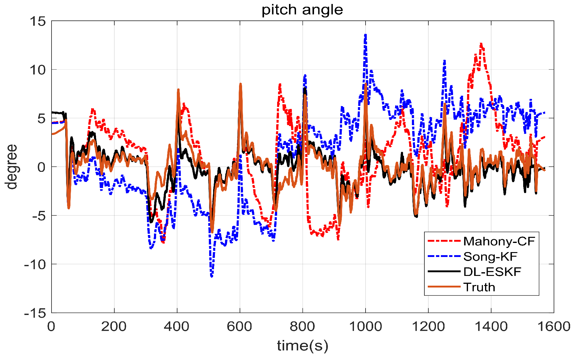
The effectiveness of the proposed algorithm in this paper was verified by simulation, and then the actual flight verification was performed on the self-developed flight control hardware as shown in Figure 18. The attitude changes of the UAV were sent to the ground station in real-time through digital transmission to observe the correctness of the solution values.

There are many parts of UAVs in the flight control system (FCS), and these include sensors of perception, remote control, ground station, and PWM rotors. The UAV FCS sets a task list of different calling frequencies, as shown in Figure 19, to ensure steady operation.

4.4. Dynamic Test

If the multi-rotor UAV maneuvering amplitude is too large, this will cause a loss of control during the flight so that the dynamics of the proposed algorithm cannot be tested. Therefore, the UAV is first stationary in the direction of the south horizontal plane, then it is held for a large-scale operation, and finally, it is stationary in the direction of the south horizontal plane.

It can be seen from Figure 20 that after a large-scale operation, and then placing the UAV in the south horizontal plane, the roll angle, pitch angle, and yaw angle can quickly converge to the initial attitude values. We demonstrated that the proposed algorithm can meet the needs of UAV flying at a large-scale operation.

4.5. Autonomous Flight Test

The UAV will fly autonomously after setting the waypoint and flight speed on the UAV ground station. The flight path is shown in Figure 21.

In this paper, the multirotor UAV was used in the autonomous flight. The flight speed was slower than the fixed-wing UAV, and the changes in attitude were also smaller than the fixed-wing UAV. The changes in attitude solution were relatively stable in the Figure 22. The reason why the yaw angle continued changing from 200 s to 600 s in Figure 23 is that when the UAV was flying from one waypoint to another, it adjusted the nose direction of the UAV. At this time, the calculated yaw angle value constantly changed in real time.

5. Conclusions and Future Work

In this paper, we presented a new weakly-coupled double-layer error Kalman filter attitude estimation algorithm to provide the reliable and steady attitude solution during small UAV real-time flight. For the small UAV short-range navigation application, a low-cost gyroscope/accelerometer/magnetometer attitude error mathematical model was designed. A double-layer ESKF attitude algorithm was proposed to solve the coupling phenomenon of the attitude sensor data due to the different sampling frequencies. The proposed DL-ESKF attitude algorithm was verified in simulation compared with the other attitude algorithms under the static and dynamic conditions of the UAV. In addition, we tested on large-scale operations and autonomous flight, which provided good attitude solution values. Future work will study the impact of harmful acceleration and wind speed on the attitude solution accuracy when the flight velocity is faster for the fixed-wing UAV, to design a more robust and reliable attitude algorithm.

References

1. Wang, C.; Wang, J.; Shen, Y.; Zhang, X. Autonomous navigation of UAVs in large-scale complex environments: A deep reinforcement learning approach. IEEE Trans. Veh. Technol. 2019, 68, 2124–2136. [Google Scholar] [CrossRef]
2. Xiong, L.; Xia, X.; Lu, Y.; Liu, W.; Gao, L.; Song, S.; Han, Y.; Yu, Z. IMU-based automated vehicle slip angle and attitude estimation aided by vehicle dynamics. Sensors 2019, 19, 1930. [Google Scholar] [CrossRef] [Green Version]
3. Koksal, N.; Jalalmaab, M.; Fidan, B. Adaptive linear quadratic attitude tracking control of a quadrotor UAV based on IMU sensor data fusion. Sensors 2019, 19, 46. [Google Scholar] [CrossRef] [PubMed] [Green Version]
4. Kamata, H.; Kimishima, M.; Sawada, T.; Suga, Y.; Takeda, H.; Yamashita, K.; Mitani, S. MEMS Gyro Array Employing Array Signal Processing for Interference and Outlier Suppression. In Proceedings of the 2020 IEEE International Symposium on Inertial Sensors and Systems (INERTIAL), Hiroshima, Japan, 23–26 March 2020; pp. 1–4. [Google Scholar]
5. Zotov, S.; Srivastava, A.; Kwon, K.; Frank, J.; Parco, E.; Williams, M.; Shtigluz, S.; Lyons, K.; Frazee, M.; Hoyh, D.; et al. In-Run Navigation Grade Quartz MEMS-Based IMU. In Proceedings of the 2020 IEEE International Symposium on Inertial Sensors and Systems (INERTIAL), Hiroshima, Japan, 23–26 March 2020; pp. 1–4. [Google Scholar]
6. Wu, J.; Zhou, Z.; Gao, B.; Li, R.; Cheng, Y.; Fourati, H. Fast linear quaternion attitude estimator using vector observations. IEEE Trans. Autom. Sci. Eng. 2017, 15, 307–319. [Google Scholar] [CrossRef] [Green Version]
7. Javed, M.A.; Tahir, M.; Ali, K. Cascaded Kalman Filtering-Based Attitude and Gyro Bias Estimation With Efficient Compensation of External Accelerations. IEEE Access 2020, 8, 50022–50035. [Google Scholar] [CrossRef]
8. Lee, B.; Lee, Y.J.; Sung, S. Attitude Determination Algorithm based on Relative Quaternion Geometry of Velocity Incremental Vectors for Cost Efficient AHRS Design. IEEE Aerosp. Electron. Syst. Mag. 2018, 19, 459–469. [Google Scholar] [CrossRef]
9. Islam, M.S.; Shajid-Ul-Mahmud, M.; Islam, T.; Amin, M.S.; Hossam-E-Haider, M. A low cost MEMS and complementary filter based attitude heading reference system (AHRS) for low speed aircraft. In Proceedings of the 2016 3rd International Conference on Electrical Engineering and Information Communication Technology (ICEEICT), Dhaka, Bangladesh, 22–24 September 2016; pp. 1–5. [Google Scholar]
10. Mahony, R.; Euston, M.; Kim, J.; Coote, P.; Hamel, T. A non-linear observer for attitude estimation of a fixed-wing unmanned aerial vehicle without GPS measurements. Trans. Inst. Meas. Control 2011, 33, 699–717. [Google Scholar] [CrossRef]
11. Lai, Y.C.; Jan, S.S. Attitude estimation based on fusion of gyroscopes and single antenna GPS for small UAVs under the influence of vibration. GPS Solut. 2011, 15, 67–77. [Google Scholar] [CrossRef]
12. Marantos, P.; Koveos, Y.; Kyriakopoulos, K.J. UAV state estimation using adaptive complementary filters. IEEE Trans. Control Syst. Technol. 2015, 24, 1214–1226. [Google Scholar] [CrossRef]
13. Euston, M.; Coote, P.; Mahony, R.; Kim, J.; Hamel, T. A complementary filter for attitude estimation of a fixed-wing UAV. In Proceedings of the IEEE International Conference on Intelligent Robots and Systems, Nice, France, 22–26 September 2008; pp. 340–345. [Google Scholar]
14. Rogne, R.H.; Bryne, T.H.; Fossen, T.I.; Johansen, T.A. On the Usage of Low-Cost MEMS Sensors, Strapdown Inertial Navigation, and Nonlinear Estimation Techniques in Dynamic Positioning. IEEE J. Oceanic Eng. 2020, 1–16. [Google Scholar] [CrossRef]
15. Coviello, G.; Avitabile, G.; Florio, A. A Synchronized Multi-Unit Wireless Platform for Long-Term Activity Monitoring. Electronics 2020, 9, 1118. [Google Scholar] [CrossRef]
16. Wu, J.; Zhou, Z.; Chen, J.; Fourati, H.; Li, R. Fast complementary filter for attitude estimation using low-cost MARG sensors. IEEE Sensors J. 2016, 16, 6997–7007. [Google Scholar] [CrossRef]
17. Welch, G.; Bishop, G. An Introduction to the Kalman Filter. 1995. Available online: http://e.guigon.free.fr/rsc/techrep/WelchBishop95.pdf (accessed on 3 September 2020).
18. Meinhold, R.J.; Singpurwalla, N.D. Understanding the Kalman filter. Am. Stat. 1983, 37, 123–127. [Google Scholar]
19. Choukroun, D.; Bar-Itzhack, I.Y.; Oshman, Y. Novel quaternion Kalman filter. IEEE Trans. Aerosp. Electron. Syst. 2006, 42, 174–190. [Google Scholar] [CrossRef] [Green Version]
20. Kingston, D.; Beard, R. Real-time attitude and position estimation for small UAVs using low-cost sensors. In Proceedings of the AIAA 3rd Unmanned Unlimited Technical Conference, Workshop and Exhibit, Chicago, IL, USA, 20–23 September 2004; p. 6488. [Google Scholar]
21. Song, Y.; Weng, X.; Guo, X. Small UAV Attitude Estimation Based on the Algorithm of Quaternion Extended Kalman Filter. J. Jilin Univ. (Sci. Ed.) 2015, 53, 511–518. [Google Scholar]
22. Liu, H.; Li, Q.; Li, C.; Zhao, H. Application Research of an Array Distributed IMU Optimization Processing Method in Personal Positioning in Large Span Blind Environment. IEEE Access 2020, 8, 48163–48176. [Google Scholar] [CrossRef]
23. Coviello, G.; Avitabile, G. Multiple Synchronized Inertial Measurement Unit Sensor Boards Platform for Activity Monitoring. IEEE Sens. J. 2020, 20, 8771–8777. [Google Scholar] [CrossRef]
24. Sabatelli, S.; Galgani, M.; Fanucci, L.; Rocchi, A. A double-stage Kalman filter for orientation tracking with an integrated processor in 9-D IMU. IEEE Trans. Instrum. Meas. 2012, 62, 590–598. [Google Scholar] [CrossRef]
25. Yadav, N.; Bleakley, C. Accurate orientation estimation using AHRS under conditions of magnetic distortion. Sensors 2014, 14, 20008–20024. [Google Scholar] [CrossRef] [PubMed] [Green Version]
26. Youn, W.; Rhudy, M.B.; Cho, A.; Myung, H. Fuzzy adaptive attitude estimation for a fixed-wing UAV with a virtual SSA sensor during a GPS outage. IEEE Sens. J. 2019, 30, 1456–1472. [Google Scholar] [CrossRef]
27. Sabatini, A.M. Kalman-filter-based orientation determination using inertial/magnetic sensors: Observability analysis and performance evaluation. Sensors 2011, 11, 9182–9206. [Google Scholar] [CrossRef] [PubMed]
28. Madyastha, V.; Ravindra, V.; Mallikarjunan, S.; Goyal, A. Extended Kalman filter vs. error state Kalman filter for aircraft attitude estimation. In Proceedings of the AIAA Guidance, Navigation, and Control Conference, Portland, OR, USA, 8–11 August 2011; p. 6615. [Google Scholar]
29. Markley, F.L. Attitude error representations for Kalman filtering. J. Guid. Control Dyn. 2003, 26, 311–317. [Google Scholar] [CrossRef]
30. Yang, Y.; Liu, X.; Zhang, W.; Liu, X.; Guo, Y. A Nonlinear Double Model for Multisensor-Integrated Navigation Using the Federated EKF Algorithm for Small UAVs. Sensors 2020, 20, 2974. [Google Scholar] [CrossRef] [PubMed]
31. Wu, Z.; Yao, M.; Ma, H.; Jia, W.; Tian, F. Low-cost antenna attitude estimation by fusing inertial sensing and two-antenna GPS for vehicle-mounted satcom-on-the-move. IEEE Trans. Veh. Technol. 2012, 62, 1084–1096. [Google Scholar] [CrossRef]
32. Meier, L.; Honegger, D.; Pollefeys, M. PX4: A node-based multithreaded open source robotics framework for deeply embedded platforms. In Proceedings of the 2015 IEEE International Conference on Robotics and Automation, Seattle, WA, USA, 26–30 May 2015; pp. 6235–6240. [Google Scholar]
Figure 1. The self-designed miniature low-cost attitude sensor combination.
Electronics 09 01465 g001
Figure 2. Unmanned aerial vehicle (UAV) attitude filtering diagram.
Electronics 09 01465 g002
Figure 3. Attitude sensors data corrected commercial autopilot platform.
Electronics 09 01465 g003
Figure 4. Attitude real-time flight self-designed autopilot platform.
Electronics 09 01465 g004
Figure 5. Roll angle error under static conditions.
Electronics 09 01465 g005
Figure 6. Pitch angle error under static conditions.
Electronics 09 01465 g006
Figure 7. Yaw angle error under static conditions.
Electronics 09 01465 g007
Figure 8. Roll angle under static conditions.
Electronics 09 01465 g008
Figure 9. Pitch angle under static conditions.
Electronics 09 01465 g009
Figure 10. Yaw angle under static conditions.
Electronics 09 01465 g010
Figure 11. UAV flight path.
Electronics 09 01465 g011
Figure 12. Roll angle error under dynamic conditions.
Electronics 09 01465 g012
Figure 13. Pitch angle error under dynamic conditions.
Electronics 09 01465 g013
Figure 14. Yaw angle error under dynamic conditions.
Electronics 09 01465 g014
Figure 15. Roll angle under dynamic conditions.
Electronics 09 01465 g015
Figure 16. Pitch angle under dynamic conditions.
Electronics 09 01465 g016
Figure 17. Yaw angle under dynamic conditions.
Electronics 09 01465 g017
Figure 18. UAV hardware system.
Electronics 09 01465 g018
Figure 19. UAV software system.
Electronics 09 01465 g019
Figure 20. Dynamic flight attitude changes.
Electronics 09 01465 g020
Figure 21. Autonomous flight path.
Electronics 09 01465 g021
Figure 22. Autonomous flight roll angle and pitch angle.
Electronics 09 01465 g022
Figure 23. Autonomous flight yaw angle.
Electronics 09 01465 g023