An Efficient Smoke Detection Algorithm Based on Deep Belief Network Classifier Using Energy and Intensity Features

Abstract

Smoke detection plays an important role in forest safety warning systems and fire prevention. Complicated changes in the shape, texture, and color of smoke remain a substantial challenge to identify smoke in a given image. In this paper, a new algorithm using the deep belief network (DBN) is designed for smoke detection. Unlike popular deep convolutional networks (e.g., Alex-Net, VGG-Net, Res-Net, Dense-Net, and the denoising convolution neural network (DNCNN), specifically devoted to detecting smoke), our proposed end-to-end network is mainly based on DBN. Indeed, most traditional smoke detection algorithms follow the pattern recognition process which consists basically feature extraction and classification. After extracting the candidate regions, the main idea is to perform both smoke recognition and smoke-no-smoke region classification using static and dynamic smoke characteristics. However, manual smoke detection cannot meet the requirements of a high smoke detection rate and has a long processing time. The convolutional neural network (CNN)-based smoke detection methods are significantly slower due to the maxpooling operation. In addition, the training phase can take a lot of time if the computer is not equipped with a powerful graphics processing unit (GPU). Thus, the contribution of this work is the development of a preprocessing step including a new combination of features—smoke color, smoke motion, and energy—to extract the regions of interest which are inserted within a simple architecture with the deep belief network (DBN). Our proposed method is able to classify and localize reliably the smoke regions providing an interesting computation time and improved performance metrics. First, the Gaussian mixture model (GMM) is employed to capture the frames containing a large amount of motion. After applying RGB rules to smoke pixels and analyzing the energy attitude of smoke regions, extracted features are then used to feed a DBN for classification. Experimental results conducted on the publicly available smoke detection database confirm that the DBN has reached a high detection rate that exceeded an average of 96% when tested on different videos containing smoke-like objects, which make smoke recognition more challenging. The proposed methodology provided high detection ratios and low false alarms, and guaranteed robustness verified by evaluations of accuracy, F1-score, and recall for noisy and non-noisy images with and without noise.

1. Introduction

Damage caused by forest fires to vegetation, animals, and humans can have disastrous consequences for nature. The danger of forest fires is real and poses a threat to people, animals, and plants. Each summer, many countries suffer from the impacts of large forest fires.

Protection from these dangers using video images for smoke and fire detection is a challenging task for a surveillance system. The presence of smoke can be the first indication of a fire since all fires produce smoke. The main idea of the smoke detection method that we propose hereafter is essentially based on a deep learning technique called the deep belief network (DBN) [1,2]. In addition, a large number of algorithms have recently been developed to ensure reliable prediction of smoke detection. Although some progress has been made in smoke detection, most algorithms are only effective in the rapid detection of wildfires. The features extracted from smoke images can cause false alarms and the smoke detection process is slow. Conventional smoke detectors are not ideally suited to effective smoke detection because they do not specify the size, location, or direction of the smoke. Compared to video-assisted smoke detection, conventional smoke detectors provide a significant lack of information. Thus, it is necessary to develop new visual smoke detection systems with a better detection rate.

In general, smoke detection is carried out in two main phases. First, it is necessary to define the target regions, extracted using the Gaussian mixture model (GMM) [3,4,5], optical flow [6], or background subtraction [7]. Furthermore, smoke is generally characterized by both static and dynamic characteristics. The second step consists of choosing certain characteristics (such as color, motion, energy/flicker analysis, and texture) and grouping them into multidimensional feature vectors. These vectors will be classified with different classification techniques, such as: The support vector machine (SVM) machine vector support [8,9], Markov model [10], and Bayesian classifiers [11]. This classification is a crucial step to calculate and separate regions with and without smoke in the studied images. Although many methods can be applied in ideal visual conditions, some are not suitable for forest fires, as there may be reflections of sunlight and other moving objects [3,4,5]. Many researchers have proposed several avenues for the development of intelligent smoke detection systems using video cameras [12]. These methods are intended for the visible area for which the distance between the camera and the target is less than 100 m. Recently, researchers have also used infrared cameras to detect smoke which involves a high cost compared to visual domain cameras. Most proposed smoke detection methods follow the same approach as that detailed previously. Following the extraction of smoke candidate regions, researchers use a set of selected features. The greater the number of features, the more complex the method, hence the need to insert high-performing classifiers.

Zhao et al. [13] extracted the flutter feature to perform classification using the Cost Sensitive Adaboost algorithm. Feature extraction from candidate regions is established by analyzing spatial and temporal characteristics of smoke videos. All of the extracted features are combined into a single input vector used in the Cost Sensitive Adaboost algorithm. The candidate smoke regions are extracted and updated to detect motion regions. Zhao et al. selected the flutter feature and computed the flutter direction angle to label the centroid motion of candidate regions. Using this approach, the direction of the centroid from bottom to top shows the presence of smoke regions. In addition, the presence of smoke is marked by a small change of high frequency information. Then, a threshold is applied to the neighborhood of each pixel based on the center value and the result is considered a binary number. The local binary pattern extracts both dynamic and appearance features of dynamic textures and is used to compute the pattern on each block of the considered frame. This method improves the performance of smoke detection but several potential improvements could be made to extract more effective flutter features [13]. Xiong et al. [14] extracted other features: background subtraction, flicker frequency, and contours. For further assessment, they classified smoke regions by the criteria of perimeter and area of smoke sequence. This method is one of the first smoke detection methods applicable to open spaces. The limitation of this method is that the extracted smoke feature is seldom adaptive to the background scene. In addition, the dataset used cannot be used to efficiently evaluate and compare the performance [14]. Toreyin et al. [15] investigated appropriate features such as the energy behavior of regions with and without smoke. The input frames were divided into sub-images using discrete wavelet transform [16]. This is a crucial step to calculate the energy ratio and, hence, determine the energy behavior. The energy of the input frame is compared to a reference frame used as a background model. Moving objects are detected using background estimation. Additionally, for further assessment the authors used the criterion of color detection. The decrease of U and V in Luminance and chrominance YUV space in a grayish scene is a sign of the presence of smoke. This not only identifies smoke features but also allows flicker frequency computing. Finally, all of these features were combined to make a final decision using a hidden Markov model (HMM) [10].

A novel Bayesian approach is developed by Calderara et al. [17] to detect smoke regions in a scene analyzing image energy through the wavelet transform coefficients and color information. The Bayesian classifier is employed on energy and color information. They developed a statistical model of gray image energy to compare the color of the input frame and the color of the chosen reference frame. This technique detects any change of energy image in the scene [11]. In the work of Yuanbin [18,19], the quality of the image is firstly enhanced by fuzzy logic, then it is adopted to extract dynamic regions from video frames. A swaying identification algorithm based on centroid calculation is used to distinguish candidate smoke regions from other dynamic regions. The support vector machine classifier is employed after that to classify the input vector of extracted static and dynamic features. This method is reliable, but it needs a high computational time in the processing stage. Similarly, Favorskaya et al. [20] applied the basic traditional spatial and temporal features used in other methods. The traditional features describing the spatial ones are color, energy, transparency, and shape, while the temporal ones are motion, flicker, and frame difference estimator [18,19].

Visual saliency detection developed by Xu et al. [21] focused on the most important object regions in an image. The pixel-level and object-level salient convolutional neural networks are combined to extract the informative smoke saliency map [21]. The saliency map is added to the deep feature map to predict the existence of smoke in an image. Unlike popular deep convolutional networks (e.g., Alex-Net, VGG-Net, Res-Net, and Dense-Net, and the DNCNN specifically devoted to detecting smoke), the proposed end-to-end network developed by Gu et al. [22] is mainly composed of dual channels of deep sub-networks. The first one connects multiple convolutional layers and max-pooling layers. The first sub-network extracts the detailed information of smoke, such as texture. In the second sub-network, they inserted two important components. The first avoids the vanishing gradient and improves feature propagation. The second reduces the number of parameters and solves the over-fitting problem. Based on the augmented data obtained by rotating the training images, smoke detection using the denoising convolutional neural network (DCNN) can stably converge to a perfect performance [21]. To overcome the shortfalls of the existing methods, we have decided in the present work to use smoke videos captured in the visual domain by low-cost cameras and we have improved the smoke detection by implementing a powerful classifier. The smoke regions will be classified using deep belief network (DBN) [1,2], to have the probabilities of smoke and no-smoke presence in the studied frames. The DBN uses a combination of three selected features: smoke color, motion, and image energy. Furthermore, we propose to extract the movement in the different images while eliminating static images. Thus, the proposed method allows us to localize the smoke regions in each frame, contrarily to existing methods above-mentioned, which can only detect the existence of smoke regions.

The present paper is organized as follows. The different smoke features proposed in previous works are described in Section 2. Then, we present the methodology of the proposed technique in Section 3. The experimental results of the proposed method are reported and discussed in Section 4. Finally, conclusions and perspectives are presented in the last section.

2. Review of Smoke Features and Classifiers

2.1. Review of Some Smoke Features

2.1.1. Smoke Motion

Labeling smoke motion is the first step to extract candidate regions to determine the nature of motion (ordinary or chaotic). Motion detection could be realized by these techniques: background subtraction [7], and optical flow [6]. The most known and efficient technique for background subtraction is the Gaussian mixture model [3,4,5], which iteratively subtracts the background image from the current frame to find finally the moving objects. In this approach, the camera is stationary. Each pixel in the frame is defined with a mixture of K-Gaussian distributions. The probability that a pixel represents the intensity is defined with:

$$P(I_t)={\displaystyle \sum _{i=1}^K{w}_i\gamma (}{I}_t,{\mu }_i,{\sigma }_i^2)$$

(1)

where $w_i$ is the weight, ${\mu }_i$ is the mean, ${\sigma }_i^2$ is the covariance for the ith distribution and $\gamma$ is a Gaussian probability density function.

2.1.2. Smoke Color Feature

Color detection is one of the used criteria for smoke detection. The color of the smoke can be gray, white, black, or dark gray. Color features can be treated in different spaces (RGB, YUV, YCbCr, etc.). The smoke RGB and YUV rules are defined as [11]:

$$\mathrm{for}RGB,\{\begin{array}{l}r=\frac{R}{R+G+B},g=\frac{G}{R+G+B},b=\frac{B}{R+G+B}\\ r+g+b=1\end{array}$$

(2)

$$\mathrm{for}YUV,\{\begin{array}{l}Y>S_y\\ \left|U-128\right|<S_u& \left|V-128\right|<S_v\end{array}$$

(3)

where S_y, S_u, and S_v are the experimentally selected thresholds.

2.1.3. Smoke Energy

The temporal behavior of smoke is defined with the study of the energy wavelet analysis. Noting that I_t is the current frame and B_k is the background image, many studies prove that the decrease in the energy ratio in the current frame E(B_k, I_t) divided by the background energy E(B_k, BG_t) can be a pertinent characteristic of the smoke transparency, because smoke gradually softens the edges in an image. Researchers apply the discrete wavelet transform [16] to the current frame I_t and the background image Bk, before the appearance of the smoke to compute the energy with:

$$E(B_k,I_t)={\displaystyle \sum _{m,n\in B_k}L{H}^2(m,n)+H{L}^2(m,n)+H{H}^2(m,n)}$$

(4)

If the energy ratio $\alpha (B_k,I_t,B{G}_t)$ < 1, then it is a sign of the smoke presence in the frame as shown in the following equation:

$$\alpha (B_k,I_t,B{G}_t)=\frac{E\left(B_k,I_t\right)}{E(B_k,B{G}_t)}\{\begin{array}{ll}<1& Smoke\\ >1& NoSmoke\end{array}$$

(5)

Discrete wavelet transform DWT [16] creates four images: the horizontal high band/vertical high band HH, the horizontal low band/vertical high band LH, the horizontal high band/vertical low band HL, and the horizontal low band/vertical low band LL after convolving the intensity image by filter banks. The frame I_t is divided into blocks with arbitrary size. The contribution of Lee et al. [23] is the choice of the technique of clustering called boosted random forests (RBF) [24] for the smoke and no-smoke regions. This classifier offers better performance than the SVM classifier. Furthermore, Lee et al. [23] combine temporal and spatial features (color, moving object, flicker/energy analysis, disorder analysis, etc.) and insert them in feature vector for clustering to finally find smoke regions.

2.1.4. Smoke Disorder

Disorder is a dynamic feature that defines the direction and propagation of smoke, which is considered a chaotic phenomenon. It is defined with:

$$Disorder(i,j)=\frac{Perimeter(i,j)}{Area(i,j)}$$

(6)

where Perimeter(i,j) and Area(i,j) are the perimeter and the area of object i in the jth frame, respectively. The dynamic features of the smoke like area and perimeter disorder of segmented smoke region are calculated for differentiating between smoke and non-smoke region. Once the smoke features are fixed as required in each method, the smoke and no-smoke regions are classified using different types of adequate classifiers.

2.2. Smoke and No-Smoke Classification Regions Methods

Various techniques of classification are applied to feature vector to separate smoke and no-smoke regions, such as the support vector machine [8,9], Bayesian classifiers [11], and Markov models [10]. Most researches used the support vector machine [8,9] as a classification method intended for a multidimensional feature vector. Recently, researchers have reduced the number of features and inserted a better classifier for smoke detection. The comparative study between approaches is based on the criterion of detection rate of smoke frames presented as:

$$\mathrm{Detection}\mathrm{Rate}=\frac{\mathrm{number}\mathrm{of}\mathrm{positive}\mathrm{detected}\mathrm{frames}-\mathrm{number}\mathrm{of}\mathrm{false}\mathrm{detected}\mathrm{frames}}{\mathrm{number}\mathrm{of}\mathrm{smoke}\mathrm{frames}}$$

(7)

Some of the currently used methods techniques intended for smoke detection are shown in

Table 1. State of art of smoke detection methods.

Paper	Color Feature	Moving Object	Energy/Flicker Analysis	Disorder Analysis	Smoke Flutter	Classification (SVM, KNN, HMM…)
Toreyin [15] (2006)	YUV	✖	✖	✖	-	✖
Xiong [14] (2007)	-	✖	✖	✖	-	-
Zhao [13] (2015)	RGB	✖	✖	-	✖	✖
Yuanbin [19] (2016)	-	✖	-	-	-	✖
Yini [26] (2017)	RGB	✖	-	-	-	DNCNN
Hu [27] (2018)	RGB	✖	-	-	-	CNN
Pundir [28] (2019)	RGB	✖	-	-	-	Deep CNN
Proposed method	RGB	✖	✖	-	-	DBN

and detailed in our published paper [25]. Researchers in forest smoke detection have recently tried to minimize the features and insert a higher performing classifier to get the best values of detection rate. The added value of our proposed method is to implement a method that helps us to detect smoke with an optimized number of features. A simple comparison between classical smoke detection methods and our implemented method is able to demonstrate the superiority of our method in terms of detection rate and time detection. In the following, we expose our methodology based on the classification with a DBN classification.

3. Proposed Methodology

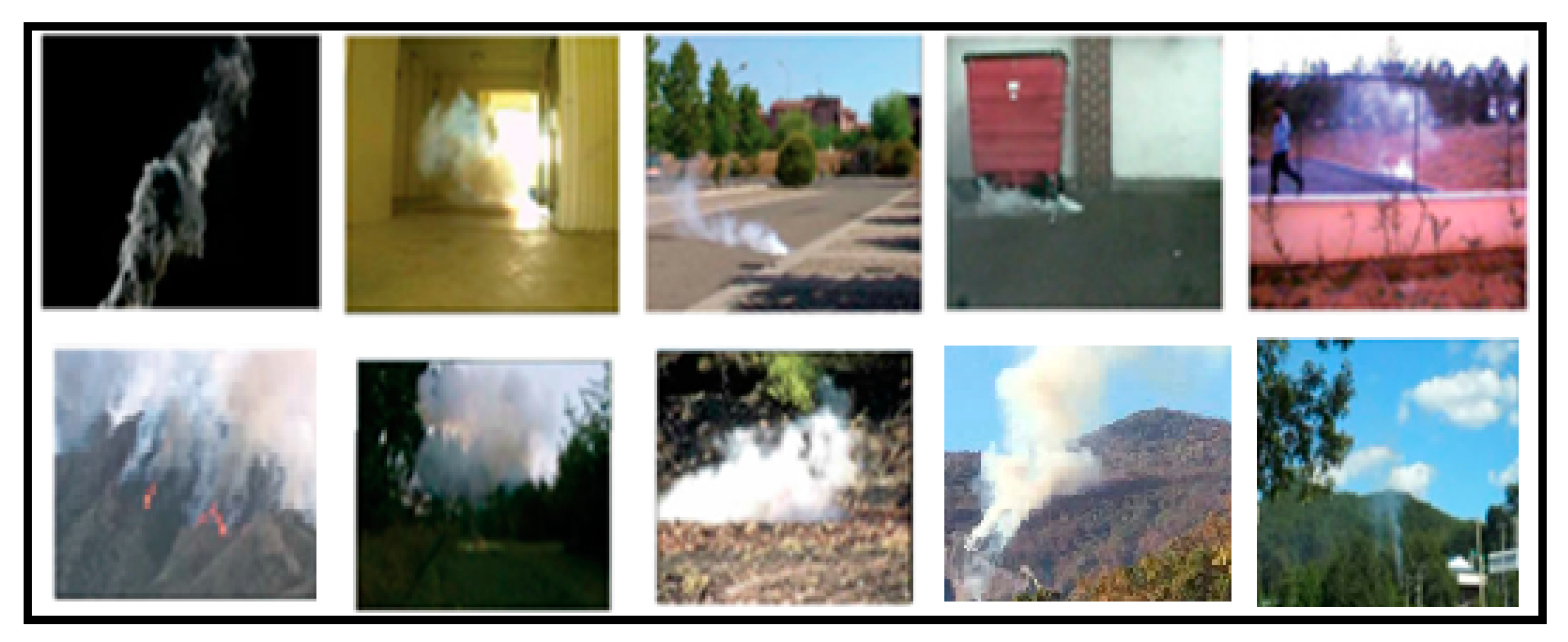
3.1. Dataset Presentation and Proposed Methodology Description

The proposed program was achieved using Python and an open source computer vision library Open CV. The used dataset is available at [29]. First of all, we divided the video into frames. The training set is used to fit the models while the validation set is used to estimate prediction errors for model selection. In order to estimate how well our model has been trained, we evaluated model properties (mean error for numeric predictors, classification errors, recall, and precision for classifiers). The training of DBN requires a lot of computation and a large number of patterns. For the training, we used a data set of ten videos containing smoke and six videos without smoke. Some frames of these videos are shown in Figure 1, Figure 2 and Figure 3. We utilized 70% of the extracted frames for training, whereas the remaining frames have been used for the test.

At this stage, we extracted frames from smoke-based videos. The size of each frame of the videos is set to 320 × 240 pixels. We used a total of 20,000 frames with equal distribution of non-smoke and smoke classes. The general idea of our work is simple. The pre-processing that we proposed to apply on the database enormously reduces the complexity of the detection method.

The main idea of our work is to select the frames containing a movement by using GMM. We eliminated the static frames. We calculated the difference between the components R, G, B of each frame. For the frames where R, G, B (experimental thresholding) are close, we kept them. We calculated the ratio of the energies for each frame and a reference frame before the appearance of the smoke. If the contours are blurred, the energy ratio is less than 1. Therefore, we kept the smoke frame and extracted the regions of interest. These regions of interest were then inserted in a vector, which was provided to the DBN network. The proposed method presented a high performance metric with an interesting computation time (detection rate, precision F1 score, accuracy, recall) with the capability of localization of smoke regions. The proposed smoke detection method is detailed by the flowcharts of Figure 4 and Figure 5.

To the best of our knowledge, the only research paper using DBN and dealing with smoke detection is Pundir’s one [28]. The difference between the proposed approach and the method developed in [27] is that we are interested only by color, motion, and energy features, and we inserted these features on the DBN classifier contrarily to the aforementioned method [28] based on motion, color, and texture analysis. For this reason, we propose, in this paper, to show the importance of using energy as a relevant smoke feature in the classification framework by comparing the performances of both methods. In addition, we think that Pundir’s algorithm is more complex than our approach in terms of feature computation since it requires, in addition to color and motion, texture analysis in each processed frame, by evaluating the local extrema co-occurrence patterns (LECoP).

The LECoP gives texture and intensity features by extracting the local directional information by the use of gray level co-occurrence matrix. Consequently, we believe that the computation of this matrix to extract textural attributes will increase the processing time of the video, and that this will present a significant problem when the scheme is implemented on real-time devices for wildland forest fire detection. The old works do not mention the true location of smoke, and do not specify the regions of interest and balance the frames as they are. The real contribution is to limit the regions of interest before feeding them into the DBN and calculating the intersection over union (IoU) criterion.

3.2. Pre-Processing of Smoke Images

The frames containing smoke are characterized by closed R, G, B components. The idea is to set an experimental threshold where R-G, R-B, G-B are close to zero. After applying the RGB rules on the foreground objects containing high motions using Gaussian mixture model as presented in Figure 6, we compute the ratio of the energy between the current frame and the energy of the background frame before the apparition of the smoke. The contours of the smoke regions become blurred. Consequently, the energy of the frames containing the smoke regions decreases. If the ratio between the energy of the actual frame and the background image is less than 1, the possibility of smoke is detected.

For this step, we used the discrete wavelet transform to obtain the HH (high-high), HL (high-low), LH (low-high), LL (low-low) sub-bands. The energy ratio is computed as shown in Equation (5).

The proposed methodology is based essentially on the choice of characteristics such as color, movement, and energy, to specify the regions of interest and locate the smoke by the trained DBN.

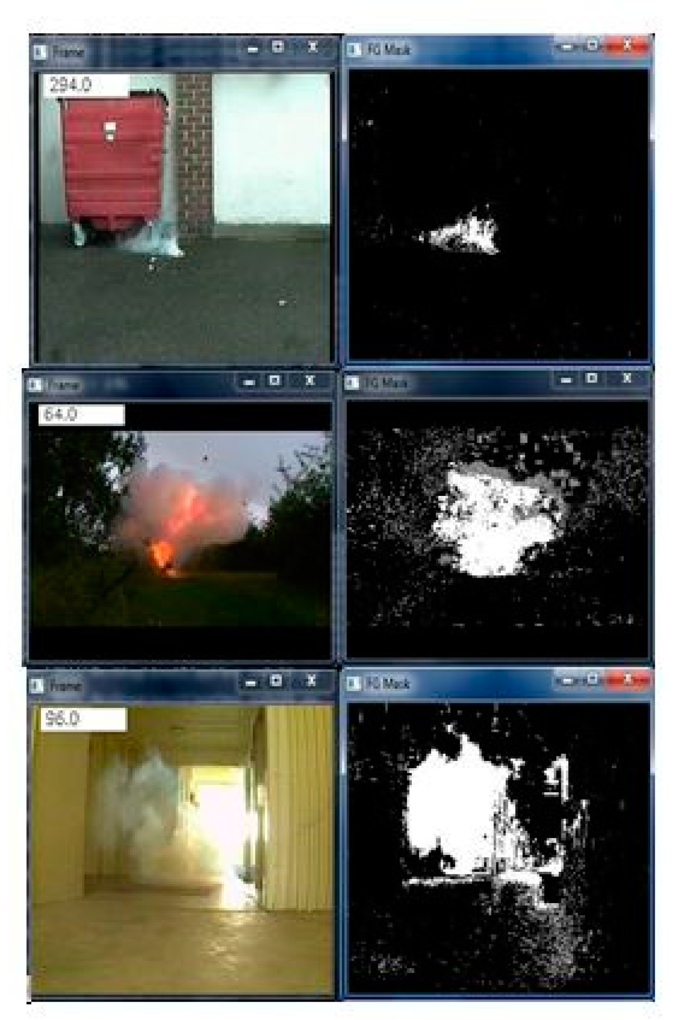
3.3. Localization of Smoke Regions

In this work, the chaotic movement of smoke is analyzed using GMM tools [3,4,5] to extract regions of high motion. We added to this criterion the color feature calculated from the matrix difference between the R, G, and B components and the energy ratio. This approach led us to easily locate the smoke in the video frames. The region of smoke is shown by a green rectangle in Figure 7.

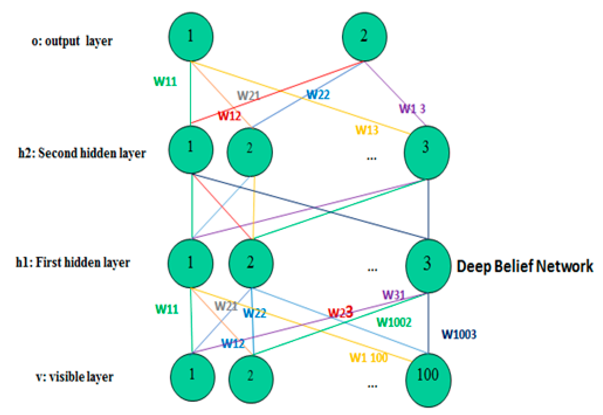
3.4. The Use of the Deep Belief Network

The deep belief network [1,2] is a probabilistic generative model compound from many layers of hidden variables. Each layer is associated to high order correlations. The generative approach is to model the joint distribution of observed and latent variables typically using a log-likelihood based criterion. This approach does not require a labeled data. The DBN used to learn our data is composed of one visible layer and two hidden layers. In addition, it is fully connected and it has 100 nodes per layer. Indeed, the DBN is a stacked restricted Boltzmann machine (RBM), which learns the features (pre-training phase) and then propagates them to fine-tune the networks. After the pre-training, our network acts like a multi-layer perceptron (MLP). Finally, after adding an output layer, we insert a logistic regression as a classifier. In the following, we present the different training steps.

3.4.1. The Pre-Training and Feature Extraction

The RBM [30,31] created by G.Hinton [2], is an algorithm suitable for classification, dimensionality reduction, feature learning. It can be considered as the basic structure block of deep-belief networks. The RBM is usually used as feature extractors and a stand-alone non-linear classifier, as well as logistic regression [32] and SVMs [8,9,33]. Each visible node takes a low-level feature from an item in our dataset to be learned. The hyper-parameters of our used network are detailed in

Table 2. Details of the hyper-parameters of the used deep belief network (DBN) network.

Hyper Parameter	Designation
vi = {1, 2, …,100}	Value of node i in the visible layer
hj = {1, 2, 3}	Value of node j in the hidden layer
b = {b1, b2, b3, …, b100} c = {c1, c2, c3}	bi, cj: bias associated with the ith visible node and jth hidden node, respectively.
$w_{ij}$	The weight between the visible units i and hidden units j
${\sigma }_i^2$	the covariance for the ith distribution
batch	64
Size of hidden layer	2

.

The energy E(v,h) used to fine tune the network model defined as

$$E(v,h)={\displaystyle \sum _{i=1}^{100}\frac{{(v_i-b_i)}^2}{2{\sigma }_i^2}}-{\displaystyle \sum _{j=1}^3{c}_j{h}_j-{\displaystyle \sum _{i=1}^{100}{\displaystyle \sum _{j=1}^3\frac{v_i}{{\sigma }_i}{h}_j{w}_{ij}}}}$$

(8)

The energy-based probabilistic models define a probability distribution through the energy function, and it is given by:

$$P(v)=P(v|h)={\displaystyle \sum _{h}p(v|h)}=\frac{1}{Z}{\displaystyle \sum _h{e}^{-E(v,h)}}$$

(9)

where

$$Z={\displaystyle \sum _{v,h}{e}^{-E(v,h)}}$$

(10)

For the training, a loss function depending on the energy aforementioned is defined as follows: The training network consists to update the parameters of the network (weight and biases) in the direction of the gradient.

Thus, this approach learns the best model for $\log P(h^{(i)},W^{(i+1)})$ by maximizing $\log p(v)$. It enables us to reduce the Kulback-Leibler divergence [34,35]. The loss function depends on the energy function and it is defined with:

$$\ln L(\theta |v)=\ln p(\theta |v)=\ln \frac{1}{Z}{\displaystyle \sum _h{e}^{-E(v,h)}}=\ln {\displaystyle \sum _h{e}^{-E(v,h)}}-\ln {\displaystyle \sum _{v,h}{e}^{-E(v,h)}}$$

(11)

where $\theta (W,b,c)$ represents the hyper parameters of the model.

The derivate term of $\frac{\partial }{\partial \theta }\ln L(\theta |v)$ called gradient, have positive and negative phases as shown

$$\frac{\partial }{\partial \theta }\ln L(\theta |v)=\ln p(\theta |v)=\ln \frac{1}{Z}{\displaystyle \sum _h{e}^{-E(v,h)}}=\frac{\partial }{\partial \theta }(\ln {\displaystyle \sum _h{e}^{-E(v,h)})}-\frac{\partial }{\partial \theta }(\ln {\displaystyle \sum _{v,h}{e}^{-E(v,h)}})$$

(12)

The positive and negative phase doesn’t refer to their signs but the reflection of the probability density defined with the model. The first term increases the probability of training data (by reducing the corresponding energy), while the second decreases the probability of generated samples. Thus, we obtain the following equation for training

$$\frac{\partial \ln p(v)}{\partial w_{ij}}={\langle v_i{h}_j\rangle }_{data}-{\langle v_i{h}_j\rangle }_{reconstructed}$$

(13)

where i = 1, …, 100, j = 1, 2, 3, and the symbols ${\langle \rangle }_{data}$ and ${\langle \rangle }_{reconstructed}$ are used to represent the expected values of the data and the reconstructed model, respectively.

This leads to a simple learning rule for performing stochastic steepest ascent in the log probability of the training data presented by

$$\Delta w_{ij}=Lr\left({\langle v_i{h}_j\rangle }_{data}-{\langle v_i{h}_j\rangle }_{reconstructed}\right)$$

(14)

where $Lr$ is the learning rate.

This parameter will be fixed in the following section. It depends on the attitude of pre-training cost per epoch. Gibbs sampling is a crucial step for training intended for sampling the system. We can start with a random state in one of the layers, and then perform alternating Gibbs sampling [36]. All the units in one layer are updated in parallel given the current state statistics of units in the other layer and this is repeated until the system is sampled. This step is the same as generating data from the infinite belief net. Gibbs sampling reduces the Kullback-Leibler divergence [34,35]. Samples of P(x) can be obtained by running a Markov chain [33] to have finally the convergence using Gibbs Sampling. Thus, the visible units are sampled simultaneously with hidden values (vice versa) as follows:

$$\{\begin{array}{l}{h}^{(n+1)}=sigm(w^{\prime }{v}^{(n)}+c)\\ v^{(n+1)}=sigm(w^{\prime }{h}^{(n+1)}+b)\end{array}$$

(15)

where, v, h are conditionally statistically independent. The terms $h^{(n+1)}$ and $v^{(n+1)}$ are randomly chosen to be 0 or 1 with the respective probabilities:

$$\{\begin{array}{l}P(h^{(n+1))}|v^{(n)})=sigm(w^{\prime }{h}^{(n+1)}+b)\\ P(v^{(n+1)}|h^{(n)})=sigm(w^{\prime }{v}^{(n)}+c)\end{array}$$

(16)

The RBM second layer is trained on the activities of the hidden units of the first RBM layer giving the data and keeping the weight fixed. The hidden units in the second RBM level tends to have strong positive weights similar to features in the first layer. The second RBM layer extracts higher level features. After the pre-training stage using the RBM, the network operates like an MLP [34].

3.4.2. The Multi-Layer Perceptron

The multi-layer perceptron is a feedforward artificial neural network trained by a supervised learning algorithm usually employed to solve binary and multi-class classification problems. It is a compound of at least three layers of nodes. Each node represents a neuron that uses a nonlinear activation function. For the training, the MLP uses generally the backpropagation algorithm as a learning algorithm. We used a simple fully connected model. The hidden layers are firstly pre-trained by a generative restricted Boltzman machine (GRBM). The principle of greedy layer -wise unsupervised in DBN with stacks of RBM is as follows:

• Train the first layer as an RBM that models the raw input v = h₀ as its visible layer.
• Use the first layer to obtain the representation of the input (W(1), h(1)) and use h(1) as the data of the second layer.
• Fix the parameter of the second layer of features and use the samples of h as the data for training the third layer.
• Fine tune all parameters with respect for DBN log-likelihood.
• Fine tune the parameters.

After the pre-training phase, we added an output layer from the parameters of the last hidden layer. We fine-tuned the weights of the pre-trained model by continuing the backpropagation, as in the classical feed-forward neural network [37]. This technique is still used to train large deep learning networks. The principle of the backpropagation approach [37,38] is to model a given function by modifying internal weights of input signals to produce an expected output signal. It is possible to fine-tune all the layers of the DBN, as it is possible to keep some of the earlier layers fixed (due to overfitting concerns) and only fine-tune some higher-level portion of the network. Once we finished the training step, we added an output layer for the classification step by using logistic regression.

3.4.3. Classification Using Logistic Regression/Adam Optimizer

a.

Logistic Regression

The classification step is established by adding a logistic regression [32] as a classifier trained with conditional maximum likelihood estimation. We choose the parameters W that maximize the log probability of the y labels in the training data given the observations v. Logistic regression is a discriminative classifier that models the decision boundary between classes [32]. A generative model explicitly estimates the actual distribution of each class. The key idea here is to predict the probability that nodes in the input layer belong to a certain class, as shown in Figure 8. The probability is defined with

$$P(y=1|v)=f_{w_{ij}}(v)=\mathrm{logistic}(w_{ij}·v)=\frac{1}{1+e^{(-w_{ij}·v)}}$$

(17)

where i = 1, …, 100, j = 1, …, 3.

For training, we should define a loss function as

$$Loss(y_t,f_{w_{ij}}(v))=-y_t\log f_{w_{ij}}(v)-(1-y_t)\log (1-f_{w_{ij}}(v))$$

(18)

For an individual training observation v in the training set, the optimal weights are estimated with:

$$w_{ij}\leftarrow w_{ij}-\alpha \frac{\partial }{\partial w_{ij}}Loss(y,f_w(v)),i.e.w_{ij}\leftarrow w_{ij}+\alpha (y-f_{w_{ij}}(v))$$

(19)

b.

Adam Optimizer

The optimization algorithm is the main tool used for training a machine learning model to minimize its error rate. Therefore, there are two metrics to determine the robustness of this algorithm: the speed of convergence and generalization on new data. Algorithms such as adaptive moment estimation (Adam) [39,40], or stochastic gradient descent (SGD) can cover one or the other metric for optimization.

Adam is an optimizer intended for gradient-based optimization of stochastic objective functions. It combines the advantages of two SGD extensions: root mean square propagation (RMSProp) [40] and adaptive gradient algorithm (AdaGrad) and calculates individual adaptive learning rates for different parameters. Despite the widespread popularity of Adam, we noted that it fails to converge to an optimal solution under specific settings as extreme learning rate and even intermediate learning rate values. The comparison between these two optimizers is then presented, showing its influence on the variation of accuracy and the cost function in Figure 9a,b. That is why we later opted to use SGD. As perspectives, we will use an optimizer that combines the speed of Adam and the capability of generalization as SGD.

4. Experimental Results and Discussion

4.1. The Network Parameters Tuning

In the present work, we extend our method previously reported in [25] by improving its performance and using a larger database containing more smoke and no-smoke videos. The following performed simulations helped us to fix the parameters of our network. Fixing the network hyperparameter enables us to have a robust network with the best results. We had also to fine-tuned the different parameters: the learning rate Lr, the number of hidden layers, and the number of pre-training epochs. We tested several values of the learning rate and we opted for Lr = 0.0006.

The difference between epoch and iteration is that epoch describes the number of times the algorithm sees the entire data while iteration describes the number of times a batch of data passes through the algorithm. Each time the algorithm goes through all the samples in the dataset, an epoch has completed. The variation of pre-training loss according to the number of epochs is shown in [23]. In addition, the number of pre-training epochs is one of the parameters for training. We tested many values of epochs and noted the time of pre-training Tp.

To have the best results for training, we should have the lowest time for pre-training with a decreasing cost function and the highest value of detection rate Dr. In our experiments, we have achieved the lowest value of pre-training time matching to the number of epochs, which is equal to 100. There is no specific number of hidden layers to obtain the best results. This number is determined by testing and noting the variation of the training cost function over the epoch and modifying in each epoch (h = 2, h = 3, h = 4).

After fixing the learning rate and the number of pre-training epochs, we have to fix the number of hidden layers, which is one of the most important parameters to pre-train the neural network. We tested a various number of hidden layers to control the attitude of the reconstruction cost of pre-training as shown in Figure 10. We tested various numbers of layers to note the influence of the number of hidden layers on the pre-training processing time Tp, on the fine-tuning processing time Tf and the detection rate. It is a crucial step to test the efficiency of the developed method with the chosen number of the hidden layers. Compared to our simulations presented in [25], we have improved the pre-training and fine-tuning time, which should be optimized by opting an appropriate number of hidden layers and pre-training epochs.

The training time process that represents the sum of the pre-training process time Tp and the fine-tuning process time Tf varies from 90 s 130 s for various tests. In addition, the time for the pre-training and the fine-tuning processing increases, whereas the detection rate decreases, if we add more than two hidden layers to our network.

After testing various numbers of layers, we notice that the loss function converges after 100 epochs. Consequently, we trained the network using SGD algorithm with momentum, and then with Adam Optimizer on 64 mini-batches for over 400 epochs. We choose to train the data with 400 epochs, the dataset will be divided into 400 subsets, and the weights will be updated maximally 400 times. The L2 weight cost on the softmax layer is fixed at 0.1. To prevent overfitting and to achieve good results, a noise is added to the inputs. In order to demonstrate the performance of the implemented network, we show in Figure 11 the variation of the detection rate according to epochs for the learning model and the validation model.

4.2. The Detection Rate and Loss Analysis

The loss per epoch is determined according to the training and validation data sets. Its interpretation depends on how well the model is doing for these two sets. The better the model, the lower the loss. The loss does not represent a percentage contrary to accuracy. It is defined with the summation of the errors made for each example in training or validation sets. The variation of the loss function of training and validation depending to the epoch are illustrated in the Figure 11a,b. The loss function is the negative log-likelihood and residual sum of squares for classification and regression respectively. The first objective in a learning model is to minimize the training loss function’s value with respect to the model’s parameters by changing the weight vector values through the backpropagation algorithm.

The loss function implies how well or poorly a certain model behaves after each iteration of optimization. Subsequently, the accuracy of our model is usually determined when the parameters have been learned and fixed. Afterwards, the test samples are provided to the model and the number of mistakes is recorded when compared to the true targets. These tests are presented in Figure 11.

4.3. Training and Validation Using the Proposed Method on the Studied Database

In the present section, several datasets are selected from the easiest to the most difficult in terms of classification. Then, the smoke and no-smoke samples are classified with the proposed method mentioned above, in Section 3.

Table 3. Results of testing the proposed method on some videos containing smoke, fogs or clouds. (M1: method of Yuanbin [18]; M2: the proposed method).

		True Positive Frames		True Negative Frames		Accuracy%		Precision%		Recall%		F1 Score		Time Processing	IoU
	Total Number of Frames	M1	M2	M1	M2	M1	M2	M1	M2	M1	M2	M1	M2	M2	M2
Test 1	275	210	225	14	23	82	90	89	94	88	93	0.88	0.93	0.6	0.85
Test 2	483	439	457	15	7	94	96	95	99	94	96	0.94	0.97	0.68	0.92
Test 3	123	104	109	6	3	89	91	94	97	93	94	0.93	0.95	0.43	0.87
Test 4	888	784	829	32	5	92	94	96	98	92	96	0.94	0.97	0.82	0.91
Test 5	808	731	762	20	14	93	96	96	99	95	96	0.95	0.97	0.76	0.94
Test 6	466	408	435	12	8	90	95	95	99	93	95.5	0.94	0.97	0.65	0.93
Test 7	626	536	560	27	10	90	91	90	92	98	99	0.93	0.95	0.71	0.88
Test 8	214	160	174	30	19	89	90	90	91.5	95	97	0.92	0.94	0.44	0.87
Test 9	507	400	430	36	21	86	90	88	91	95	96	0.91	0.93	0.68	0.89
Test 10	304	0	0	291	298	95	98	0	0	0	0	-	-	0.48	-
Test 11	109	0	0	102	104	93	95	0	0	0	0	-	-	0.31	-
Test 12	84	0	0	79	81	94	96	0	0	0	0	-	-	0.29	-

contains the results of testing on a set of 12 videos containing smoke, fogs or clouds. In order to show the effectiveness and the robustness of the proposed method, the tested videos are chosen as follows: the first six tests in the database represent videos containing only smoke. The next three tests are videos containing clouds, fogs, and moving people. The last three tests illustrate videos without smoke. We notice here that there is no standard database for smoke detection. Therefore, our proposed method of smoke detection is compared to the work of W. Yuanbin [18], noted M1, aforementioned in the state of the art, and which uses the SVM as a classifier. The results of the comparison are illustrated in Table 3, on the same database, where the accuracy, precision, recall, F1 score values are presented. The accuracy is defined with

$$\mathrm{Accuracy}=\frac{TP+TN}{TP+TN+FP+FN}$$

(20)

$$\mathrm{Precision}=\frac{TP}{TP+FP}$$

(21)

$$\mathrm{Recall}=\frac{TP}{TP+FN}$$

(22)

$$\mathrm{F}1\mathrm{Score}=2\frac{\mathrm{Precision}·\mathrm{Recall}}{\mathrm{Precision}+\mathrm{Recall}}$$

(23)

where TP is the true positive frames, TN is the true negative frames, FP is the false positive frames and FN is the false negative frames.

In addition, the intersection over union (IoU) metric is reported in Table 3 as an evaluation of smoke localization provided by the proposed segmentation method. It is the area of overlap between the predicted segmentation (Spred) and the ground truth (Strue), divided by the area of union between these two segmentations:

$$IoU=\frac{Strue\cap Spred}{Strue\cup Spred}$$

(24)

The IoU ranges from 0–1 (0–100%), with 0% signifying no overlap and 100% signifying perfectly overlapping segmentation. This metric evaluates the localization of smoke regions. The time processing of smoke detection using the proposed method is also presented in Table 3. Indeed, Table 3 shows that the first six tests containing only smoke have fairly high smoke detection values, ranging from 90% to 96% using the proposed method (M2). Moreover, for videos containing only smoke, the accuracy for the method (M1) is balanced in the margin (82–94%). For the three tests containing smoke, moving people, or cloud we found that the presence of objects causes a decrease in the detection rate. The smoke detection values in these cases are ranging from 89% to 91%. For the last three tested videos that do not contain smoke, the methods do not detect smoke and the detection values are then zero. In this case, the accuracy and the detection rate depend essentially on the true negative frames and false positive frames in the absence of smoke in videos. As shown in the obtained results, and after several tests comparing to the three smoke detection methods, our proposed method, generally have the highest number of true positive frames and the lowest true negative frames. The presence of constraints as moving people, fogs, or clouds increases the number of true negative frames. Consequently, the detection rate and accuracy decrease compared to videos with smoke only. Additionally, the time processing of the videos containing smoke varies between (0.43–0.82 s) depending, essentially, on the total number of frames, number of hidden layers, and nodes.

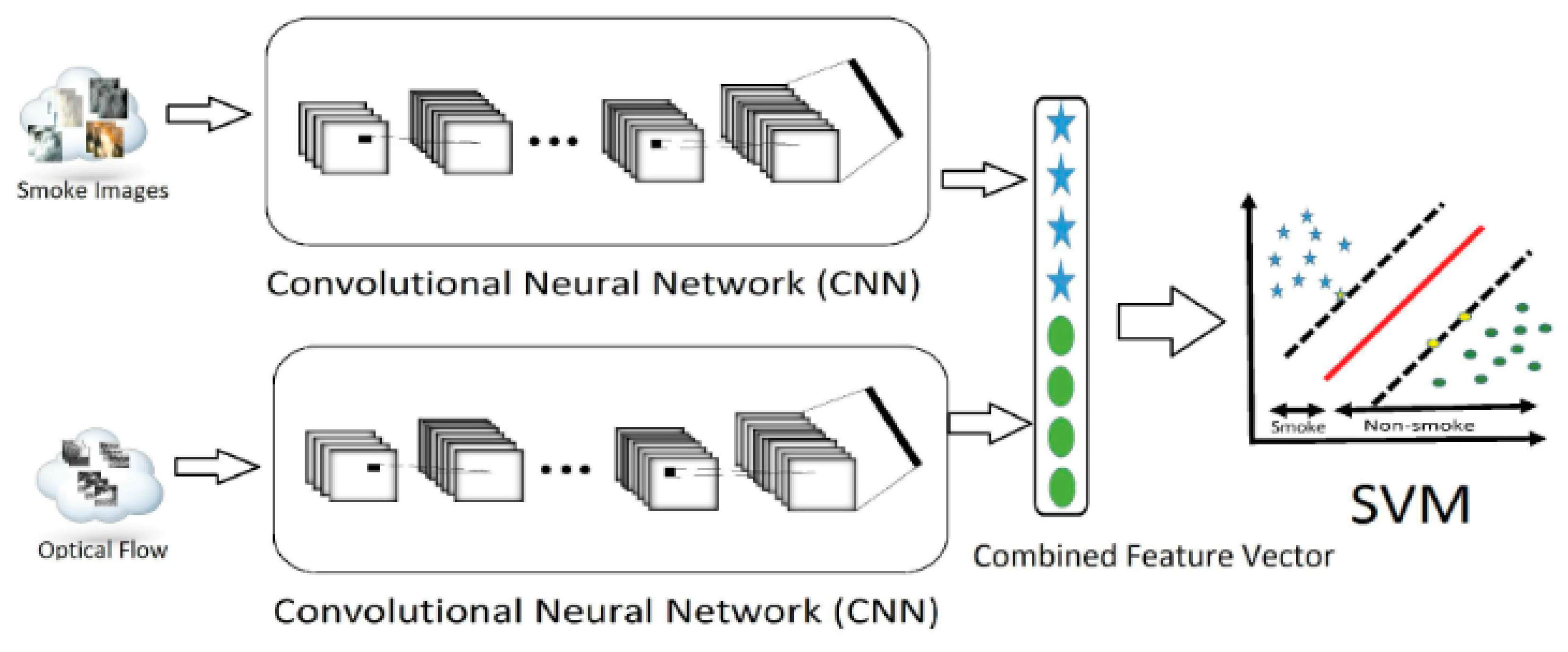
4.4. Comparison of Smoke Detection Results Using Support Vector Machine and Deep CNN

In the smoke detection method based on SVM [8,9,19,33], smoke regions are extracted by the Gaussian mixed model. Then static and dynamic features are extracted. The characteristics vectors are then classified by the SVM, for smoke recognition, after fixing the hyperparameter of the SVM. This method will be compared with our proposed method on the same dataset. We use the SVM referring to the smoke detection method developed by Yuanbin [18], on the same data, with texture features as inputs.

Furthermore, knowing that the deep CNN used by Pundir et al. [28] remains the best alternative for smoke detection, the performances of the proposed method are compared to [28] in this section. Our goal is not to beat the robustness criteria values achieved by this method, but to propose an alternative for smoke detection with a simpler architecture. The deep CNN based method extracts smoke features using two deep learning frameworks and tries to classify smoke and non-smoke region.

The first deep learning framework is used super pixel algorithm to extract smoke features (color, texture, disorder, sharp edge, etc.). The second-deep learning framework is employed for computing smoke motion feature after applying the optical flow [41] to capture the chaotic motion of smoke. Features extracted from both frameworks are presented to deep CNN and are combined to train the SVM [33].

The training process of the deep CNN method is summarized in Figure 12 [28]. Unlike this method, in our proposed technique of smoke detection, we only insert the chosen feature vector for classification using DBN to directly obtain the smoke and no-smoke probabilities (Figure 5). Apart from the complexity of the method developed in [28], this method requires a large amount of data to have good classification results and the time of training process takes a lot of time, especially if the computer is not equipped with a good GPU. On the other hand, the proposed smoke detection method does not require so much data to have a good classification rate, and it is able to locate the smoke before classifying the smoked and non-smoked areas.

4.5. Robustness of the Proposed Method in the Noisy Case

The present work is analyzed by a challenging smoke dataset. Despite the higher performance of this method, it gets affected by the presence of noise as clouds and moving people, which slightly decreases the detection rate in some cases.

Thus, we will test the robustness of the implemented work reverts to adding noise to the inputs and notice the attitude of the detection process. In fact, noise is traditionally added to the inputs, but it can also be added to weights, gradients, and even activation functions.

Furthermore, this approach makes the input space smoother and easier to learn. Additionally, adding noise during the training can make the training process more robust and reduce generalization error. Furthermore, adding noise expands the size of the training dataset. Consequently, adding noise to input samples is a simple form of data augmentation. At first, we propose to add Gaussian noise to test the robustness of the proposed method. This allows us to use variance-stabilizing methods on smoke inputs. The results of the additive noise are presented in

Table 4. The accuracy results for different Gaussian noise levels.

SNR	Accuracy
1 dB	87.5%
5 dB	93%
20 dB	94.5%

. The noise level is quantified by the signal to noise ratio (SNR) value [42] calculated with:

$$SNR=20\log \frac{\mathrm{var}(Input)}{\mathrm{var}(Noise)}$$

(25)

Three levels of noise are added to the inputs: low noise (SNR = 20 dB), medium noise (SNR = 5 dB), and high noise (SNR = 1 dB).

Finally, to show the difference between the aforementioned classifiers, we apply these methods on videos containing smoke (without moving people and fogs), and we calculate the following classical criteria: accuracy, precision, recall, F1 score defined in Equations (20)–(23), and the time of training process for each method. The results of this experiment are shown in

Table 5. Comparison of recent smoke detection methods for the studied video set with noise and without noise.

Condition	Classifier	Accuracy	F1 Score	Precision	Recall	Time of Training Process (s)
Without Noise	SVM	0.93	0.95	1	0.91	135
	Deep CNN	0.97	0.98	1	0.96	100
	Proposed DBN	0.96	0.97	1	0.95	60
With Gaussian Noise SNR 5 dB	SVM	0.91	0.95	0.91	1	168
	Deep CNN	0.95	0.97	0.94	1	115
	Proposed DBN	0.93	0.96	0.92	1	84

. The obtained values of recall, precision and F1 score show that the robustness proposed method. In addition, the criteria values are very close to calculated values using the deep CNN classifier, but represent better values than the SVM classifier, even in the presence of noise.

The difference between our developed technique and the deep CNN classification technique is that, through our method, we can easily localize the smoke regions with a feature vector fed into simple architecture after extracting smoke features: motion, color, and energy analysis. This advantage obviously allows us to classify smoke zones more easily and rapidly than the deep CNN classifier.

In fact, the deep CNN models [28] found in the literature for smoke detection are usually very deep, with many layers and inspired by models dealing with several classes’ classification.

Moreover, deep CNN requires a lot of computation time, as well as a lot of data that is sometimes not easily available. The DBN has historically demonstrated their usefulness through Hinton’s work in the 2000s [1,2], and has been successfully used for classification problems.

The deep CNN based method extracts smoke features using two deep learning frameworks and classifies smoke and non-smoke regions. This aforementioned technique requires a high computation time.

Our proposed method uses a generative model combined with logistic regression. Additionally, unlike CNN-based methods, which are fully supervised, we have moved towards a semi-supervised approach, in which we exploit the ability of DBN to obtain a high level hierarchical representation of the tested data.

The proposed method ensures important values (accuracy, precision, F1 recall) compared with smoke detection techniques based on SVM treated in the state of the art. Apart from this advantage, we can locate and classify regions of interest at the same time and we have calculated IoU as a smoke localization criterion, which was not treated in the works mentioned in the state of the art. The real value of our work is to locate and classify regions of interest with interesting values of performance, and the computation time and resources needed for training and testing, without forgetting that the main purpose of smoke extraction is to locate and classify, with a minimum of execution time and resources and high performance metrics.

After using many assessment criteria, we concluded that the proposed method is far more effective than any other widely used methods for smoke detection, owing to its robustness and accuracy. Exceptionally, the proposed method yields good classification and detection results, especially in a noiseless condition. In the presence of noise, these results are slightly affected.

5. Conclusions

In this paper, a novel smoke detection and localization technique is proposed by combining different smoke features: color, motion, and energy. Contrarily to up-to-date methods, we prepare our inputs for training to localize the smoke regions and also to classify smoke and no-smoke regions using a DBN classifier. In addition, the proposed system can be used for real-time smoke detection. The calculated time processing on our dataset varies from (0.43–0.82 s), essentially depending on the total number of frames, number of hidden layers, and nodes.

The advantages of the proposed method with respect to other smoke detection methods can be summarized in two points. The first one is the easy and fast localization of the smoke regions, with an IoU changing from 0.85 to 0.94 for videos containing smoke regions. Smoke detection using the proposed method can easily and rapidly localize and classify smoke and no-smoke regions, compared to the conventional smoke detection methods and deep CNN that requires a lot of computation time, as well as a lot of data, which is sometimes not easily available. In addition, we have worked on challenging database by adding to smoke and no-smoke videos another input, containing moving people, clouds, and fogs. Compared to most smoke detection methods using deep CNN [28], the proposed method has the highest values of detection rate, which can reach 96%, even in a noisy context. We conclude that our method is more reliable than many other methods and can provide a high detection rate. Moreover, the capacity of treating a huge number of frames is a real advantage of this approach. In future works, we can propose the use of a dual DBN to improve the detection rate and the smoke localization in each frame. As perspectives, we will use an optimizer that combines the speediness of Adam and the capacity of generalization on new data as SGD. A possible improvement to the developed system is the incorporation of AdaBound to substantially improve the detection rate and more images to train the network for higher accuracy.

References

1. Hinton, G.E.; Osindero, S.; Teh, Y.-W. A Fast Learning Algorithm for Deep Belief Nets. Neural Comput. 2006, 18, 1527–1554. [Google Scholar] [CrossRef] [PubMed]
2. LeCun, Y.; Bengio, Y.; Hinton, G. Deep Learning for Single Image Super-Resolution: A Brief Review. Int. J. Sci. Nat. 2015, 521, 436–444. [Google Scholar]
3. Yang, J.; Yuan, X.; Liao, X.; Llull, P.; Brady, D.J.; Sapiro, G.; Carin, L. Video Compressive Sensing Using Gaussian Mixture Models. IEEE Trans. Image Process. 2014, 23, 4863–4878. [Google Scholar] [CrossRef] [PubMed]
4. Viswanath, A.; Behera, R.K.; Senthamilarasu, V.; Kutty, K. Background Modelling from a Moving Camera. Procedia Comput. Sci. 2015, 58, 289–296. [Google Scholar] [CrossRef] [Green Version]
5. Huang, M.; Chen, G.; Yang, G.-F.; Cao, R. An Algorithm of the Target Detection and Tracking of the Video. Procedia Eng. 2012, 29, 2567–2571. [Google Scholar] [CrossRef] [Green Version]
6. Mahfouf, Z.; Merouani, H.F.; Bouchrika, I.; Harrati, N. Investigating the use of motion-based features from optical flow for gait recognition. Neurocomputing 2018, 283, 140–149. [Google Scholar] [CrossRef]
7. Santoyo-Morales, J.E.; Hasimoto-Beltrán, R. Video Background Subtraction in Complex Environments. J. Appl. Res. Technol. 2014, 12, 527–537. [Google Scholar] [CrossRef]
8. Demidova, L.; Klyueva, I.; Sokolova, Y.; Stepanov, N.; Tyart, N. Intellectual Approaches to Improvement of the Classification Decisions Quality on the Base of the SVM Classifier. Procedia Comput. Sci. 2017, 103, 222–230. [Google Scholar] [CrossRef]
9. Hsu, C.-W.; Lin, C.-J. A comparison of methods for multiclass support vector machines. IEEE Trans. Neural Netw. 2002, 13, 415–425. [Google Scholar]
10. Bicegoa, M.; Mário, V.M.; Figueiredo, A.T. Similarity-based classification of sequences using hidden Markov models. Pattern Recognit. 2004, 37, 2281–2291. [Google Scholar] [CrossRef]
11. DeNoyer, L.; Gallinari, P. Bayesian network model for semi-structured document classification. Inf. Process. Manag. 2004, 40, 807–827. [Google Scholar] [CrossRef]
12. Kaabi, R.; Frizzi, S.; Bouchouicha, M.; Fnaich, F.; Moreau, E. Video Smoke Detection Review. In Proceedings of the 2017 International Conference on Smart, Monitored and Controlled Cities (SM2C), Sfax, Tunisia, 17–19 February 2017. [Google Scholar]
13. Zhao, Y.; Li, Q.; Gu, Z. Early smoke detection of forest fire video using CS Adaboost algorithm. Int. J. Light Electron. Opt. 2015, 126, 2121–2124. [Google Scholar] [CrossRef]
14. Xiong, Z.; Caballero, R.; Wang, H.; Finn, A.M.; Lelic, M.A.; Peng, P.-Y. Video-Based Smoke Detection: Possibilities, Techniques, and Challenges; IFPA Fire Suppression & Detection Research & Applications: East Hartford, CT, USA, 2007; pp. 1–7. [Google Scholar]
15. Toreyin, B.U.; Dedeoglu, Y.; Cetin, A.E. Contour Based Smoke Detection in Video Using Wavelets. In Proceedings of the 14th European Signal Processing Conference (EUSIPCO 2006), Florence, Italy, 4–8 September 2006; pp. 1–5. [Google Scholar]
16. Ghazali, K.H.; Mansor, M.F.; Mustafa, M.M.; Hussain, A. Feature Extraction Technique using Discrete Wavelet Transform for Image Classification. In Proceedings of the 2007 5th Student Conference on Research and Development, Selangor, Malaysia, 11–12 December 2007; pp. 1–4. [Google Scholar]
17. Calderara, S.; Piccinini, P.; Cucchiara, R. Smoke Detection in Video Surveillance: A MoG Model in the Wavelet Domain. In Computer Vision Systems; Springer Science and Business Media: Berlin/Heidelberg, Germany, 2008; Volume 5008, pp. 119–128. [Google Scholar]
18. Wang, Y. Smoke Recognition Based on Machine Vision. In Proceedings of the 2016 International Symposium on Computer, Consumer and Control (IS3C), Xi’an, China, 4–6 July 2016; Volume 283, pp. 668–671. [Google Scholar]
19. Yuan, F. A fast accumulative motion orientation model based on integral image for video smoke detection. Pattern Recognit. Lett. 2008, 29, 925–932. [Google Scholar] [CrossRef]
20. Favorskaya, M.N.; Pyataeva, A.; Popov, A. Spatio-temporal Smoke Clustering in Outdoor Scenes Based on Boosted Random Forests. Procedia Comput. Sci. 2016, 96, 762–771. [Google Scholar] [CrossRef] [Green Version]
21. Xu, G.; Zhang, Y.; Zhang, Q.; Lin, G.; Wang, Z.; Jia, Y.; Wang, J. Video smoke detection based on deep saliency network. Fire Saf. J. 2019, 105, 277–285. [Google Scholar] [CrossRef] [Green Version]
22. Gu, K.; Xia, Z.; Qiao, J.; Lin, W. Deep Dual-Channel Neural Network for Image-Based Smoke Detection. IEEE Trans. Multimed. 2020, 22, 311–323. [Google Scholar] [CrossRef]
23. Lee, B.; Han, D. Real-Time Fire Detection Using Camera Sequence Image in Tunnel Environment. In Lecture Notes in Computer Science; Springer Science and Business Media LLC: Berlin/Heidelberg, Germany, 2007; Volume 4681, pp. 1209–1220. [Google Scholar]
24. Mishina, Y.; Tsuchiya, M.; Fujiyoshi, H. Boosted Random Forest. In Proceedings of the International Conference on Computer Vision Theory and Applications, Liston, Portugal, 5–8 January 2014; pp. 594–598. [Google Scholar]
25. Kaabi, R.; Sayadi, M.; Bouchouicha, M.; Fnaiech, F.; Moreau, É.; Ginoux, J.M. Early smoke detection of forest wildfire video using deep belief network. In Proceedings of the 2018 4th International Conference on Advanced Technologies for Signal and Image Processing (ATSIP), Sousse, Tunisia, 21–24 March 2018; pp. 1–6. [Google Scholar]
26. Yin, Z.; Wan, B.; Yuan, F.; Xia, X.; Shi, J. A Deep Normalization and Convolutional Neural Network for Image Smoke Detection. IEEE Access 2017, 5, 18429–18438. [Google Scholar] [CrossRef]
27. Hu, Y.; Lu, X. Real-time video fire smoke detection by utilizing spatial-temporal ConvNet features. Multimed. Tools Appl. 2018, 77, 29283–29301. [Google Scholar] [CrossRef]
28. Pundir, A.S.; Raman, B. Dual Deep Learning Model for Image Based Smoke Detection. Fire Technol. 2019, 55, 2419–2442. [Google Scholar] [CrossRef]
29. Cetin, A.E.; on behalf of the Bilkent SPG Signal Processing Group. Computer Vision Based Fire Detection Software. Available online: http://signal.ee.bilkent.edu.tr/VisiFire/index.html (accessed on 10 May 2020).
30. Hrasko, R.; Pacheco, A.G.C.; Krohling, R.A. Time Series Prediction Using Restricted Boltzmann Machines and Backpropagation. Procedia Comput. Sci. 2015, 55, 990–999. [Google Scholar] [CrossRef] [Green Version]
31. Zhang, N.; Ding, S.; Zhang, J.; Xue, Y. An overview on Restricted Boltzmann Machines. Neurocomputing 2018, 275, 1186–1199. [Google Scholar] [CrossRef]
32. Efron, B. The efficiency of logistic regression compared to Normal Discriminant Analysis. J. Am. Stat. Assoc. 1975, 70, 892–898. [Google Scholar] [CrossRef]
33. Maruta, H.; Nakamura, A.; Kurokawa, F. A novel smoke detection method using support vector machine. In TENCON 2010–2010 IEEE Region 10 Conference; Institute of Electrical and Electronics Engineers (IEEE): Piscataway, NJ, USA, 2010; Volume 431, pp. 210–215. [Google Scholar]
34. Carreira-Perpinan, M.A.; Hinton, G.E. On contrastive divergence learning. In Proceedings of the Artificial Intelligence and Statistics (AISTATS), Bridgetown, Barbados, 6–8 January 2005; pp. 1–8. [Google Scholar]
35. Hinton, G.E. Training Products of Experts by Minimizing Contrastive Divergence. Neural Comput. 2002, 14, 1771–1800. [Google Scholar] [CrossRef] [PubMed]
36. Chou, P.-H. A Gibbs sampling approach to the estimation of linear regression models under daily price limits. Pac.-Basin Financ. J. 1997, 5, 39–62. [Google Scholar] [CrossRef]
37. Chang, T.-C.; Chao, R.-J. Application of back-propagation networks in debris flow prediction. Eng. Geol. 2006, 85, 270–280. [Google Scholar] [CrossRef]
38. LeCun, Y.; Bottou, L.; Bengio, Y.; Haffner, P. Gradient-based learning applied to document recognition. Proc. IEEE 1998, 86, 2278–2324. [Google Scholar] [CrossRef] [Green Version]
39. Zou, F.; Shen, L.; Jie, Z.; Zhang, W.; Liu, W. A Sufficient Condition for Convergences of Adam and RMSProp. In Proceedings of the 2019 IEEE/CVF Conference on Computer Vision and Pattern Recognition (CVPR), Long Beach, CA, USA, 15–20 June 2019; pp. 11119–11127. [Google Scholar]
40. Basu, A.; De, S.; Mukherjee, A.; Ullah, E. Convergence guarantees for RMSProp and ADAM in non-convex optimization and their comparison to Nesterov acceleration on autoencoders. arXiv 2018, arXiv:1807.06766. [Google Scholar]
41. Horn, B.K.; Schunck, B.G. Determining optical flow. Artif. Intell. 1981, 17, 185–203. [Google Scholar] [CrossRef] [Green Version]
42. Neelakantan, A.; Vilnis, L.; Le, Q.V.; Sutskever, I.; Kaiser, L.; Kurach, K.; Martens, J. Adding Gradient Noise Improves Learning for Very Deep Networks. arXiv 2015, arXiv:1511.06807. [Google Scholar]
Figure 1. The environments and samples of smoke video database: examples of frames containing smoke.
Electronics 09 01390 g001
Figure 2. The environments and samples of smoke video database: examples of frames. Including smoke, moving people, clouds, or fogs.
Electronics 09 01390 g002
Figure 3. The environments and samples of smoke video database: examples of frames without smoke.
Electronics 09 01390 g003
Figure 4. Flowchart of the proposed algorithm for smoke detection.
Electronics 09 01390 g004
Figure 5. Smoke detection and classification using the proposed method based on the deep belief network.
Electronics 09 01390 g005
Figure 6. Some results of the background subtraction using the Gaussian mixture model (GMM).
Electronics 09 01390 g006
Figure 7. Some results of smoke regions localization.
Electronics 09 01390 g007
Figure 8. Architecture of the proposed deep belief network.
Electronics 09 01390 g008
Figure 9. (a) Comparison of stochastic gradient descent (SGD) and adaptive moment estimation (Adam) optimizer and influence on the loss function. (b) Comparison of SGD and Adam optimizer and influence on the accuracy.
Electronics 09 01390 g009
Figure 10. Variation of pre-training loss according to the number of epochs to fix the number of network hidden layer.
Electronics 09 01390 g010
Figure 11. (a) Training and validation loss function comparison on our database f. (b) Training and validation accuracy comparison on our database.
Electronics 09 01390 g011
Figure 12. Bloc diagram of the Pundir method’s (smoke detection and classification) with two deep learning frameworks) [26].
Electronics 09 01390 g012