Abstract
In recent years, the number of fraud cases in basic medical insurance has increased dramatically. We need to use a more efficient method to identify the fraudulent users. Therefore, we deploy the cloud edge algorithm with lower latency to improve the security and enforceability in the operation process. In this paper, a new feature extraction method and model fusion technology are proposed to solve the problem of basic medical insurance fraud identification. The feature second-level extraction algorithm proposed in this paper can effectively extract important features and improve the prediction accuracy of subsequent algorithms. In order to solve the problem of unbalanced simulation allocation in the medical insurance fraud identification scenario, a sample division method based on the idea of sample proportion equilibrium is proposed. Based on the above methods of feature extraction and sample division, a new training and fitting model fusion algorithm (tree hybrid bagging, THBagging) is proposed. This method makes full use of the balanced idea of the tree model algorithm based on Boosting to fuse, and finally achieves the effect of improving the accuracy of basic medical insurance fraud identification.
1. Introduction
For decades, with the growing consolidation and improvement of medical insurance of China, more than 1.3 billion people [1,2] are sharing the social dividends in the developed process. Unfortunately, fraudulent attempts to obtain medical insurance funds have continued in recent years. Basic medical insurance (the term “basic medical insurance” in this paper can be shortly denoted “medical insurance”) fraud refers to deceiving insurance personnel to obtain insurance compensation through insurance or fictitious or exaggerated insurance injuries [3]. This behavior infringes the rights of others and seriously harms social health. The behavior of those who commit medicare fraud is variable, and criminal methods are constantly emerging, which makes it difficult to identify fraud through intuitive judgment [4,5]. However, through continuous accumulation of medical insurance data, data mining [6] and machine learning [7] technologies can be used to analyze massive data to find the potential rules of fraudsters, and effectively identify the real fraudsters.
In the basic medical insurance identification scenario, traditional methods include screening of diagnosis and treatment rules [8], data comparison [9], etc. These methods have achieved certain results, but due to the relatively backward technical means, there are limitations in many aspects, including the inability to dig out the common characteristics of illegal personnel, low efficiency and low recognition accuracy and recall rate due to the need for human participation in the recognition process [10,11]. Through data mining and machine learning technology, we can achieve more efficient and intelligent identification of medical fraud. At present, the main methods used are clustering [12], decision tree [13], random forest [14], and so on. Another part of the people also achieved good results through the neural network method [15,16,17]. Compared with these commonly used algorithms, the integrated learning based on the tree model has the characteristics of fast training speed, strong generalization ability and high prediction accuracy. But in the current research, this method is rarely used in the research of medical fraud identification. In this paper, the method of integrated learning is used to construct an intelligent monitoring model of social medical insurance based on a fusion model of combinatorial classifier, so as to realize the intelligent supervision of fraudulent behaviors.
Both machine learning and integrated learning have high requirements for data sets, and a good data set can greatly improve the accuracy of experimental results [18,19,20]. However, the recognition problem based on medical insurance is a category imbalance problem. For binary classification, the ratio of positive and negative samples is not 1 to 1, but it reaches 1 to 10 or 1 to 100, which is called class imbalance. In a machine learning task, the problem brought by the imbalance of the categories is that for the categories with a relatively small distribution, the model often cannot be well trained and fitted. The main reason is that its sample size is too small, or that most of the model’s energy is used to fit more classes, while less classes are underfitted [21]. This article uses the idea of category division and equalization to process the data, which can solve the above problems well.
Another difficulty of basic medical insurance recognition is that the effective features cannot be extracted in the feature extraction stage [22]. The behavior of the insured is variable and complex. How to select useful features from many behavioral characteristics is an important basis to distinguish law-abiding person and illegal person. Neural network cannot get good classification results, a large part of the reason is caused by improper feature selection [23]. In this paper, second-level feature extraction method is innovatively proposed, which can effectively extract important features.
The key contributions of our work can be summarized as follows.
- We propose a novel idea of sample equalization to deal with the problem of category imbalance in medical insurance identification. The sample data were extracted using the combination of smote and K-means. For negative samples, we use the smote method to solve the over-fitting problem of random sampling through synthetic samples. For positive samples, we use K-means clustering algorithm to select data according to the proportion of each category.
- Aiming at the difficulty of feature selection in the basic medical insurance fraud recognition scenario, we propose a second-level feature extraction algorithm based on the classification tree model, which uses the path information represented by the leaf nodes in the tree model to compress and represent various user behavior. The result data generated by the algorithm provides data input for subsequent model training.
- This paper proposes a new model fusion algorithm (tree hybrid bagging, THBagging). The algorithm is based on the fusion of integrated learning theory and existing models. The strategy of “excellent and different” is integrated organically, which effectively improves the values of and -.
- In order to facilitate further research on this task, we publicly provide the source code and data of the model on the GitHub community as contributions to the community (The experimental details and source code of the model are publicly available at https://github.com/zhanghekai/THBagging).
The remainder of this paper is organized as follows. In Section 2, we reviewed the relevant research related to our task, and in Section 3 introduced the data set used, and proposed a solution to the imbalance of sample distribution. Section 4 provides the details that drive our proposed fusion model framework. In Section 5, we conducted extensive experimental evaluation and analyzed the effectiveness of the classification experimental results. Finally, the conclusions and future work are described in Section 6.
2. Related Work
2.1. Medical Insurance Fraud Identification
In order to identify fraud in basic medical insurance, Chen et al. [13] proposed a data mining-based medical insurance fraud identification model, which mainly uses a prediction model established by cluster analysis and classification decision tree algorithms to identify a patient whether your medical treatment is suspected of fraud. Francis et al. [24] proposed an improved support vector machine (SVM) method to identify medical insurance fraud by using medical insurance transaction records, and the results were satisfactory. Tang et al. [25] used principal component analysis and K-means cluster analysis to analyze the medical insurance industry. Fashoto et al. [12] took the medical insurance claim data of Nigeria as an example and used the K-means clustering method to group the similar samples into one class. The one with a small sample size was marked as a fraud group. The fraud was detected by looking for the outliers based on clusters. Vipula et al. [26] analyzed the advantages and disadvantages of several commonly used algorithms in supervised and unsupervised methods, and designed a hybrid model based on unsupervised clustering method and supervised support vector machine classification algorithm for fraud detection. Junhua et al. [14] used the random forest algorithm to identify the fraudulent behavior and medical insurance data to verify it. The results show that the fraud detection model has a good identification effect on the fraudulent behavior. Liou et al. [27] used data from Taiwan for analysis, and used logistic regression, decision trees, and neural networks to build a recognition model. By comparing the three methods, a suitable model was selected for prediction of fraud samples.
The above research has achieved good results, but the feature extraction mode is relatively simple, and it is impossible to effectively extract important hidden features. Most of them are interpretable features through human cognition, and these features are for the model. Training is far from enough, and it cannot improve the accuracy of the model.
Many researchers have adopted the BP neural network method to study the intelligent identification of basic medical insurance fraud. Hubick [28] from the Australian Medical Insurance Commission used a neural network algorithm to identify fraud in medical insurance. Lin Yuan et al. [15] improved the design of the neural network, and realized the improvement of the fraud recognition accuracy rate by using the three-layer neural network. Bisker et al. [16] uses the improved neural network algorithm to study the risk early warning of the new rural cooperative medical insurance fraud, and tests the simulation data. The model has a good effect on the fraud identification. Anbarasi et al. [29] uses the back propagation (BP) neural network method. In addition, a logistic regression algorithm is used to improve the neural network. Panigrahi et al. [17] uses a combination of neural network and bayesian network to identify fraud, through bayesian learning of a historical database to update the suspicion score.
In summary, in the existing researches, the common methods for intelligently identifying medical insurance frauds using data mining algorithms are machine learning, neural networks, integrated learning, etc., and have achieved certain research results [30]. However, many of the researches are theoretical researches on intelligent monitoring, and lack of real analysis data. In the empirical research on the real data of medical insurance, there are few data dimensions, mainly including the self-payment ratio, hospitalization cost, material cost and nursing cost. The algorithm used is only a single data mining algorithm or an improved data mining algorithm.
2.2. Dataset Division
In the method of solving the problem of data imbalance, Chawla et al. [31] manually defined a few samples by defining the smote method to achieve the purpose of balancing the data set, but this method is difficult to fit high-latitude samples. Based on the over-sampling smote algorithm, Liang et al. [32] proposed the LR-SMOTE algorithm.An improved over-sampling method for unbalanced data sets based on K-means and SVM to make the newly generated samples closer to the sample center, avoid generating abnormal samples or changing the distribution of the data set. In contrast to overs-ampling, Drummond et al. [33] proposed an undersampling method to achieve the relative equilibrium among categories by reducing the majority of samples, and then trained them using the traditional classification algorithm. Ribeiro et al. [34] proposed a classification method based on multi-objective integrated learning. This method performs comprehensive learning through multi-objective optimization design methods to deal with unbalanced data sets. However, the above method only reconciles from one category, and cannot process multiple categories of data simultaneously.
3. Dataset
3.1. Dataset
The data used in this article is the actual medical settlement data. The data set comes from the “Internet + Human Society” 2020 Action Plan issued by the Ministry of Human Resources and Social Security. The data set includes medical insurance medical settlement desensitization data and cost details of 20,000 insured personnel in 456 medical institutions from July 2016 to December 2016 in Hebei province, Beijing and Tianjin, China. It mainly includes the medical expense records and expense details of the insured personnel, as well as the information about whether there are any illegal behaviors of medical insurance fund fraud. Among them, there are 19,000 normal people (positive samples) and 1000 fraudsters (negative samples), and a total of 74 features are included.
3.2. Data Preprocessing
In order to eliminate noise and bias results, we preprocess the data set as follows:
Noisy Data Filtering. Denoising the basic medical insurance data is the first step in data preparation. Only based on accurate and valid data can data mining algorithms be used to accurately identify fraud and ensure the effectiveness of intelligent monitoring research on basic medical insurance fraud. We perform noise reduction on the data in three steps:
- Clean the original data. The purpose of data cleaning is to screen out the required data from the perspective of medical insurance fraud and related needs of modeling. Therefore, this step eliminates unnecessary data. Mainly includes: (a) Of all the consumption record information, 94.5% of the consumption record information does not get blood transfusion costs, so the data related to blood transfusion costs will be eliminated. (b) In the original data, there are date and time fields such as declaration acceptance time, transaction time and operation time, and in the extraction of short-term dimensions, the date and time fields are relatively important. Therefore, the date field in the data is converted to a unified standard date format.
- Deal with missing values in the original data. This paper finds that there are 3000 missing values in 13 variables. The meaning of missing values should be the amount without the item, so the missing value part of the above variables is replaced with 0, which means that the amount is zero.
- Handle the outliers of the original data. Outliers refer to data that does not conform to normal rules and has abnormalities. Considering that in the actual situation, the declared amount must be less than the amount that occurred. Therefore, this article defines the value of the declared amount of each amount greater than the occurred amount as an abnormal value. However, because it is impossible to confirm whether it is the declared amount or the abnormality caused by the amount error, and the abnormal value is rare, it is a record that does not affect other expense items, so the amount field of this fee for this record is reset to 0.
Through the above-mentioned denoising of the original data, we get neat medical insurance details, and we show all the processed features in Table 1.

Table 1.
Medical insurance data set features.
Data Splitting. This article intends to judge whether there are fraudulent violations based on the characteristics of users’ medical treatment and consumption, which is essentially a two-category problem. The processed sample data in this article contains 17,000 effective information of insured persons, of which the ratio of negative sample to positive sample is 1:16. The sample ratio is seriously unbalanced, so handling the sample imbalance problem is an important prerequisite for achieving accurate identification of fraud, and solving the sample imbalance problem is an important task of this article. In this paper, a combination of undersampling and oversampling is used to resample the sample using a hybrid method based on K-means [35] clustering undersampling and smote [36] oversampling.
For negative samples. We use the smote sampling algorithm to solve the overfitting problem of random oversampling by artificially synthesizing samples. It assumes that the samples between the fraud samples with close distance are still the fraud samples. A new fraud sample is generated randomly between the two samples with close distance through the linear interpolation method, so as to increase the synthetic fraud samples and balance the proportion of the two data samples. The smote sampling algorithm requires a given k value, calculates k nearest neighbors for each fraud sample , randomly selects a neighbor , and uses Equation (1) to generate a composite sample between and .
Among them, Rand (0, 1) is used to generate a random number between 0 and 1. Finally, add the newly generated sample to the data set. In this paper, each sample is used to generate a new fraud sample, a total of 1000 negative samples are generated, and the original negative samples are combined into a new negative sample.
For positive samples. We use K-means clustering algorithm to cluster samples with certain similarity. After K-means clustering, normal samples are divided into several clusters. According to the number of samples in each cluster, the proportion of each cluster to the population is calculated and recorded as the sampling proportion. Normal samples are randomly selected from each cluster according to the sampling proportion as new normal samples. The new normal samples contain all the information of normal samples. It should be emphasized that the purpose of clustering analysis in this process is to extract samples that are consistent with the overall sample characteristics as much as possible, not to subdivide each user in the sample. Therefore, when the number of K is determined in advance by K-means clustering, and in order to find the best K value for clustering effect, the range of K is artificially set at 5–10. Compare the interia (https://scikit-learn.org/stable/modules/clustering.html#k-means) in K-means function in Python change trend of attribute value, select the best K value. The change of evaluation index values of different clustering results is given in Figure 1.
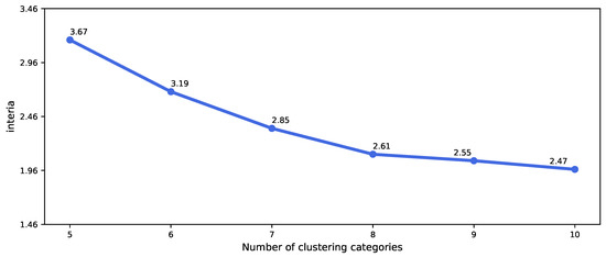
Figure 1.
Variation of interia value of different clusters.
The value of interia changes greatly when the number of classification categories is less than 8, but after being divided into 8 categories, the value of interia decreases relatively less. It shows that when all normal samples are grouped into 8 categories, the samples in the cluster are relatively similar, which is very different from the samples outside the cluster. It should be emphasized that the purpose of undersampling using clustering algorithms in this paper is to extract as many samples as possible that are consistent with the characteristics of the overall sample. Considering that when normal samples are grouped into 9 and 10 categories, the effect of interia does not change much, and the proportion of each category is not balanced, the number of normal samples included in individual categories is very small. Therefore, this article finally chose to cluster the samples into 8 categories. After the K-means clustering algorithm is used to cluster all normal insured persons into 8 categories, the sample size and proportion of each category are shown in Table 2.
Table 2.
Statistics on the sample size and proportion of each category after K-means clustering.
Sample division. We draw 2000 positive samples from each cluster according to the sampling ratio, and form a new sample with 2000 negative samples. According to this method, 5 sets of data are drawn according to the ratio without replacement, and finally the negative samples are reused to form 5 sets of new samples. The advantage of this method is to solve the problem of uneven distribution of categories, and has the advantage of oversampling, which expands the sample set. Using a variety of different models for training can also achieve the effect of reducing overfitting, and also avoid the problem of excessive data discarding in downsampling, and can make full use of the data set. Therefore, such an imbalanced sample distribution can solve the problem well.
4. The Proposed Approach
4.1. The Overall Framework
Figure 2 shows the overall framework that describes the use of the proposed THBagging model in fraud detection of medical insurance. The framework consists of two stages: model building and prediction. In the model construction stage, our goal is to build a composite classifier by using several basic classifiers constructed by the tree model classification algorithm. In the prediction stage, this fusion model classifier is used to predict whether new samples that have never appeared are fraudulent users.
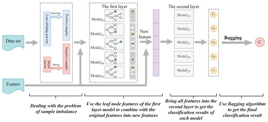
Figure 2.
The overall framework of our proposed approach.
Our framework first extracts available features from the training samples. Then, a hybrid method combining K-means clustering undersampling and smote oversampling is used to divide the samples in a balanced manner. Using this divided data, we construct a fusion classification model by combining different basic classifiers. For the feature second-level extraction, the input of the second layer in the fusion model is a combination of the leaf node features and the original features obtained by the first layer. The parameters of each part of the fusion classification model are trained and obtained. After building the fusion classifier, in the prediction stage, it is used to predict whether the new sample is a fraudulent user. From the new sample, our framework first preprocesses and extracts features. Then input these features into the fused model classifier that has been trained. Finally, the classifier outputs the prediction result: fraudulent or normal.
4.2. THBagging Model
4.2.1. The First Layer of the THBagging Model
The first layer algorithm of THBagging model uses one GBDT [37], two XGBoost [38] and two LightGBM [39], which are all algorithm models based on Boosting idea. The consideration of not using the random forest algorithm [40] in the first layer is that the first layer is mainly feature extraction and combination in feature engineering. The random forest algorithm is an integrated learning algorithm based on bagging. It mainly focuses on the variance of the fitted samples. The time is independent of each other, so after the sample falls into the leaf nodes of each decision tree, the correlation or combination type between the leaf nodes is not very strong, so as a combined feature, it will not be a very good feature. The GBDT and XGBoost models based on the Boosting algorithm are the deviations of the fitted samples. The current decision tree is fitted with the deviation of the previous decision tree, which is a continuous optimization process, so whether the sample falls between the leaf nodes of the decision tree is relevant. Another advantage is that the training data of the tree model does not require one-hot processing, which can solve the problem of sparse features.
The original data set has been divided into 5 new data sets through undersampling and oversampling methods, and the 5 new data sets are input into the five models of the first layer for training. For each model of the first layer, use the 10-fold cross-validation [41] method to find the best parameters of each model for the input data set. Finally, the important parameters of the five models of the first layer of THBagging algorithm in this paper are shown in Section 5.3.
4.2.2. Second-Level Feature Extraction
The second-level feature extraction method uses the leaf node number of the sample falling into the model as the new feature. For the tree classification algorithm, each non-leaf node is selected by a feature in the feature set for division. The prediction result of the tree classification algorithm is the linear weighting of the prediction results of each base classifier, and the prediction result of the base classifier for a sample is the result of the sample falling into the leaf node of the base classifier, then this leaf node number can be used as feature utilization. As shown in Figure 3, taking one of the tree models in the first layer of the THBagging model as an example, each subtree under the model is numbered in sequence, and the resulting sequence number is the new feature name. If there are n subtrees in the tree model, then n leaf node features can be obtained. The final sample will fall into the leaf node of each subtree. The leaf nodes of each subtree are numbered starting from 1. The number of the leaf node where the sample is located is the value of the new feature corresponding to the subtree.
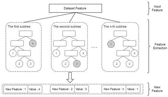
Figure 3.
Feature second-level extraction.
For example, in the GBDT algorithm, the CART regression tree is used as the base classifier. In the basic medical insurance fraud recognition scenario in this paper, it is assumed that a sample falls into a leaf node of the k regression tree, and its number is 2. The path traversed is that the number of hospitalization days is greater than 7, the number of visits in the month is greater than 10, and the amount of medicine is less than 90. The number 2 represents the above-mentioned combination feature, and k represents the name of the combination feature. If the label of this sample is 1, then these features represent the attributes of the sample with label 1. These combined features are difficult to find through artificial data mining.
Then the features generated by the second-level feature extraction and the features extracted by the primary feature are combined into a complete feature, which is used as the input of the second layer in the THBagging model.
4.2.3. The Second Layer of the THBagging Model
In this paper, the combination of the second layer and the first layer base classifier of THBagging algorithm is that the first group of models uses GBDT + RF, the second group of models uses XGBoost + LightGBM, the third group of models uses XGBoost + RF, and the fourth group of models uses LightGBM + XGBoost, the fifth group model uses LightGBM + GBDT. In this section we introduce the core part of the model used in the second layer.
The RF algorithm is used in the second layer of the first group and third group models. First, we use bootstrap method to generate m training sets. Then, for each training set, we construct a decision tree. When we split the features of node searching, we do not find all the features that can maximize the index (such as information gain), but extract a part of the features in the feature, find the optimal solution among the extracted features, and apply it to node splitting. RF algorithm adopts the idea of integration, which is equivalent to sampling samples and features, so it can avoid overfitting.
The second layer of the second group of models uses the LightGBM algorithm. We first discretize continuous floating-point eigenvalues into k integers and construct a histogram of width k at the same time. By selecting only the node with the largest split gain for splitting, the overhead caused by the smaller gain of some nodes is avoided. LightGBM’s improved binary tree splitting gain formula is:
where is the complexity cost introduced by adding new leaf nodes, and is the regular term coefficient. and are the first order derivatives of the left and right subtree sample loss functions, respectively, and and are the second order derivatives of the left and right subtree sample loss functions, respectively. is the score of the left subtree of the node to be split, and is the score of the right subtree of the node to be split.
The second layer of the fourth group of the model uses the XGBoost algorithm. When solving the extreme value of the loss function, the Newton method is used to expand the loss function to the second order. In addition, a regularization term is added to the loss function. The objective function during training consists of two parts. The first part is the loss of the gradient lifting algorithm, and the second part is the regularization term. The loss function is defined as:
where n is the number of training function samples, l is the loss of a single sample, assuming it is a convex function. is the model’s predicted value for the training sample, and is the true label value of the training sample. The regularization term defines the complexity of the model:
where and are manually set parameters, is the vector formed by the values of all leaf nodes in the decision tree, and T is the number of leaf nodes.
GBDT algorithm is used in the second layer of the fifth group of models. GBDT can find a variety of distinguishing features and feature combinations. We make multiple iterations of GBDT, and each iteration produces a weak classifier. Each classifier is trained on the basis of the residual of the previous round of classifier, and then the accuracy of the final classifier is continuously improved by reducing the deviation. Our classification tree model is:
where m is the number of samples in the data set, is the leaf node area of the m-th tree, , J are the number of leaf nodes of the regression tree m, and is the best residual fitting value. is the indicating function. If the content in parentheses holds (i.e., ), the return value is 1, otherwise the return value is 0. is the required classification tree model.
Finally, the prediction results will be determined by the vote of the classifiers of these combined models. We use the Bagging algorithm to average the output of multiple classifiers:
where T is the number of classifiers, is the weight of individual learner , we require , .
4.2.4. Feature Importance Calculation
Because the fusion model uses different tree models, in order to unify the calculation of feature importance in THBagging model, we will accumulate the degree of enhancement of a feature in the segmentation criteria in each tree split as a measure of the importance of the feature, and take the mean value on all trees, which is the relative importance of the feature [42,43]. Since the features in the medical insurance fraud identification data set are continuous values, we use the square error as the segmentation criterion [44].
The global importance of feature j is the sum of the importance of feature j in each single tree, which is measured after averaging:
where M is the number of trees and is the m-th tree. The importance of feature j in a single tree is as follows:
where L is the number of leaf nodes of the tree, and is the number of split nodes in the tree (that is, the number of non-leaf nodes, the constructed tree is a binary tree with left and right children). is the segmentation feature associated with node t. The function indicates that if the segmentation feature of node t is j, the value is 1; otherwise, the value is 0; is the reduction of the squared error after node t is split, representing the lifting degree of the segmentation criterion on node t.
5. Experiments
In this section, we first introduce the annotation of ground truth data, compared Open IE baseline methods and evaluation metrics. Then, we conduct extensive experiments to evaluate the effectiveness of our proposed major algorithms in the system. Finally, the experimental results are discussed, including: (a) analysis of candidate fact extraction, (b) analysis of running time for different methods, (c) investigation of the quality of experimental variance, and (d) comparative analysis of variant models.
5.1. Evaluation Metrics
The three metrics are applied for our evaluation, including F-measure, - and AUC-ROC.
5.1.1. F-Measure
F-measure, which is the harmonic mean of Precision and Recall, is a standard and widely used measure for evaluating classification algorithms [45]. There are four possible outcomes for an instance in a target project: an instance can be classified as law-abiding person when it actually is law-abiding person (true positive, TP), as law-abiding person when it is in fact illegal person (false positive, FP), as illegal person when it is in fact law-abiding person (false negative, FN), as illegal person when it actually is illegal person (true negative, TN). Based on these possible outcomes, the detailed definitions of Precision, Recall and are obtained as follows:
5.1.2. Macro-F
- [46] is a metric which evaluates the averaged of all the different class-labels. Let , , denote the true-positives, false-positives and false-negatives for the t- label in label set respectively. - gives equal weight to each label in the averaging process. Formally, - is defined as:
5.1.3. Area under the Receiver Operator Characteristic Curve
ROC [47] is a non-parametric method used to evaluate models. It plots the precision/recall values reached for all possible cutoff values ranging with the interval [0, 1]. Therefore, it is independent of the cutoff, different from the precision and recall metrics. A curve of the false positive rate is plotted against the true positive rate. We report the AUC-ROC [48] values. The AUC-ROC value measures the probability that a randomly chosen clean entity. An area of 1 represents a perfect classifier, whereas for a random classifier an area of 0.5 is expected.
5.2. Compared Baseline Methods
In order to evaluate our method more comprehensively, we compared a set of classic and latest baselines, as shown in Table 3:
Table 3.
Baseline algorithm comparison.
5.3. Implementation Details
All our experiments were performed on 64 core IntelXeon CPU E5-2680 v4@2.40 GHz with 512 GB RAM and 8 NVIDIA Tesla P100-PICE GPUs. The operating system and software platforms are Ubuntu 5.4.0 and Python 3.7.0. Python has a lot of open source algorithm libraries, which provides a lot of convenience for experiments. We use sklearn to import these algorithm libraries for experiments. On the one hand, the parameters of the classifier are obtained through a lot of testing and adjustment; On the other hand, they are the results of the classifier’s independent selection after training. We show various parameters used in the experiment in Table 4.
Table 4.
THBagging model parameter selection and setting.
5.4. Analysis and Comparison of Experimental Results
5.4.1. Second-Level Feature Extraction Importance Analysis
In order to verify the importance of the second-level feature extraction in Section 4.2.2, the second-level extracted features are compared with the original features, and the feature importance can be used for verification. Generally speaking, importance scores measure the value of features in the model’s promotion decision tree construction. In the research of medical insurance fraud recognition, the more attributes are used to construct a classification tree in the model, the higher its importance. If there are second-level extracted features ranked high, it proves that the second-level extracted features have a good effect.
We use the feature importance calculation formula introduced in Section 4.2.3 to obtain the importance value of each feature used. The feature importance ranking is shown in Figure 4. From the figure, it can be seen that the English names are the original features, and the numbers represent the second-level feature extraction. Seventeen of the top 20 important features belong to the second-level feature extraction feature, indicating that the second-level feature extraction effectively extracts important features.
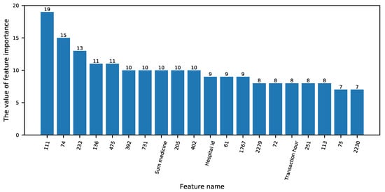
Figure 4.
Feature importance ranking.
5.4.2. Analysis of Performance Results for Different Models
Compare with baseline algorithm. From the experimental results of Table 5, the results obtained by using the fusion model are better than the methods of machine learning and neural network. The P and R of the proposed method based on integrated learning are above 70% and 45% respectively, and at least higher than the baseline algorithm 2.93% and 2% at and -. - treats all categories equally and is not easily affected by common categories. Especially in the case of imbalanced sample categories, the effect of - is better. It not only shows the superiority of the data division method, but also shows that the THBagging model is more robust in uneven samples. The proposed THBagging belongs to the fusion model, and its value and - value are higher than all the basic classification model combinations used, indicating that the concept of model fusion is successful.
Table 5.
Precision (P), recall (R) and results (%) for different models.
The ROC curve of the proposed model is shown in Figure 5, and the area under the curve represents the value of AUC, which is an evaluation index to measure the merits of the two-class model. The AUC value of the THBagging model is higher than that of all baseline algorithms, indicating that the positive examples predicted in the classification process are more likely to be ranked before the negative examples. The THBagging model has the ability to consider the classification of positive and negative examples at the same time, and can still make a reasonable evaluation of the classifier in the case of imbalanced samples.
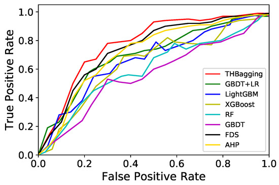
Figure 5.
Quantitative analysis of model fusion.
The THBagging algorithm is integrated by multiple tree model algorithms, and each tree model algorithm is calculated in parallel, so its time complexity is the same as the tree model is O (tree depth × tree of tree). Because the THBagging algorithm is a fusion algorithm, it is slower than other single-model algorithms. Regarding the prediction time, because the THBagging algorithm is an offline algorithm, it is very close to the prediction time of other models in the experiment, and the prediction time of the offline algorithm is not high, so it is completely within the acceptable range.
It can be seen from the experimental results in Table 6 that the proposed model experimental results have a small variance in and -, indicating that the algorithm results are universal and there are no abnormal phenomena such as fluctuations, which provides a guarantee for the subsequent analysis of algorithm results. It can be seen from Figure 6 that in each group of experiments, the correlation coefficient matrix shows that the correlation coefficient of the five combined models in THBagging algorithm is not large and the correlation between the models is not high. On this basis, the model can produce better results.
Table 6.
The variance () of performance results for different models.
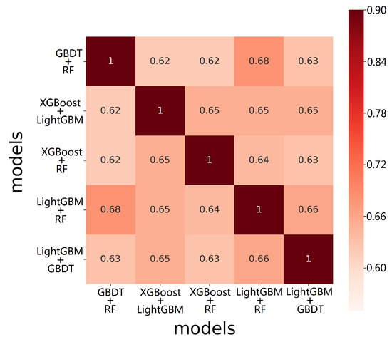
Figure 6.
Correlation coefficient matrix of the tree hybrid bagging (THBagging) model.
Compare with the variant model.
—THBagging: In order to verify the superiority of the tree model classifier, we change the second layer of the model into a common classification algorithm. Here the second level classification algorithm uses SVM [51], KNN [52], DT [53] and LR [54]. In order to keep consistent with the combination times of THBagging model, we still conducted experiments with five sets of arbitrarily matched models, and the best results after several experiments are shown in Table 5. The best combinations were XGBoost + SVM, XGBoost + KNN, GBDT + LR, LightGBM + DT and LightGBM + LR. According to the experimental results, the experimental results using the tree model are better, because the tree model can choose more important features for classification. From the Table 6, it can be seen that the ordinary classifier has a large variance, which reflects that the THBagging algorithm does not have good stability.
—THBagging: We use existing data processing methods to balance the problem of large differences in the number of positive and negative samples, and compare it with our proposed equalization method (smote + K-means). The comparative data processing methods used here include SMOTE [31], LR-SMOTE [32] and MOEL [34]. In order to reflect the rationality of the experiment, we only adjusted the data processing in the following experiments, and the experimental model remained consistent. We show the test results in the Table 7. No matter what kind of evaluation index, the data balancing method we proposed has reached the highest value. and - are at least 2.76% and 2.48% higher than the baseline algorithm. This is because the existing data balancing methods only deal with data from one aspect, that is, increase or decrease the number of a category, which obviously cannot achieve a good data balance. We consider the problem of data balance from multiple categories at the same time.
Table 7.
Comparison of data balance processing methods.
—THBagging: In order to verify the influence of different times of model fusion on the experimental results, we conducted a comparative experiment with model combination times of 3, 4, 5, 6, 7. In the process of modifying the model combination, we remove the base model with many classification errors and add a new base model. According to the above THBagging experiment, it is meaningless to add the same model combination, so we randomly add a new set of model combinations, and show the best experimental results of different combination times in Table 8. It can be seen from the table that the performance of THBagging achieves the best performance with the increase of fusion times when fusion times are 5. Since then, THBagging’s performance has deteriorated, possibly due to overfitting, with too many results fed into the Bagging algorithm, reducing the final accuracy of the model. This is also an important reason why our THBagging model chooses the number of combinations to be 5.
Table 8.
Model fusion experiment.
—THBagging: In order to verify the superiority of model combination diversity, we used five groups of the same combination model as the basic model for the experiment. With the remaining conditions unchanged, we conducted five experiments with the same base model as THBagging, and compared with a single base model. The experimental results are shown in Figure 7. From the figure we can see that the THBagging model approximates, or does not improve, the experimental results of a single base model. This makes sense because the same model treats the test data as a category, which is equivalent to running the same model five times and feeding it into the Bagging algorithm, which makes no sense.
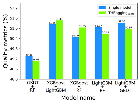
Figure 7.
Comparison of the same model combination with a single model.
—Number of layers stacked: In order to find the optimal number of layers for model stack, we experimented with models with different number of layers. The experimental results are shown in Figure 8. When the number of stacked layers is 2, the model gets the best experimental results. When the number of layers is 1, the model does not integrate the original features with the leaf nodes, which makes the experimental precision insufficient. As the number of stacked layers increases, the accuracy of the model starts to decline. This is because from the second layer, the input feature of each layer is the fusion of the previous layer feature and the original feature. The higher the number of layers, the greater the input feature will be. We show the optimal stacking conditions used in the experiment in Table 9.
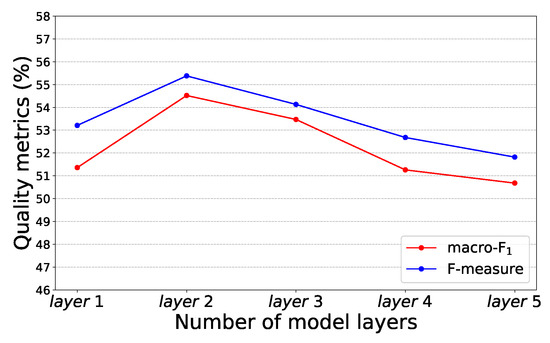
Figure 8.
Comparison of experimental results under different layers.
Table 9.
Hierarchical stacking experiment.
6. Future and Conclusions
In this paper, the intelligent identification problem of basic medical insurance fraud is analyzed and discussed. According to the problem scenario, detailed and in-depth feature analysis and extraction are performed through data analysis and mining, and two rounds of feature extraction are performed based on the traditional feature extraction mode. Aiming at the problem of imbalanced category distribution in the basic medical insurance fraud recognition scenario, the THBagging algorithm was first proposed. This algorithm was used to solve the problems of insufficient sample utilization, easy overfitting, and low recognition rate in the category distribution problem. Finally, through the research content of this article, it is proved on the experimental data that THBagging algorithm is better than traditional algorithms.
In the future, we plan to study the adaptive feature ranking semantic algorithm based on natural language understanding (NLP) to improve the problem of feature importance screening and analysis.
Author Contributions
Conceptualization, J.G.; Data curation, H.Z. and W.D.; Investigation, W.D.; Methodology, H.Z.; Writing—original draft, H.Z. All authors have read and agreed to the published version of the manuscript.
Funding
This paper was partially supported by National Natural Science Foundation of China (Nos.61572111 and 61876034).
Acknowledgments
The authors would like to thank the support of the laboratory and university.
Conflicts of Interest
The authors declare no conflict of interest.
References
- Zhu, S.; Wang, Y.; Wu, Y. Health care fraud detection using nonnegative matrix factorization. In Proceedings of the 2011 6th International Conference on Computer Science & Education (ICCSE), Singapore, 3–5 August 2011; pp. 499–503. [Google Scholar]
- Zhiwei, L.; Yingtong, D.; Yutong, D.; Hao, P.; Philip, S.Y. Alleviating the Inconsistency Problem of Applying Graph Neural Network to Fraud Detection. arXiv 2020, arXiv:2005.00625. [Google Scholar]
- Liu, C.; Zhu, X.Y. Medical Insurance Fraud Identification Based on BP Neural Network. Comput. Syst. Appl. 2018, 27, 34–39. [Google Scholar]
- Xu, W.; Wang, S.; Zhang, D.; Yang, B. Random rough subspace based neural network ensemble for insurance fraud detection. In Proceedings of the 2011 Fourth International Joint Conference on Computational Sciences and Optimization, Yunnan, China, 15–19 April 2011; pp. 1276–1280. [Google Scholar]
- Yali, G.; Xiaoyong, L.; Hao, P.; Bingxing, F.; Yu, P.S. HinCTI: A Cyber Threat Intelligence Modeling and Identification System Based on Heterogeneous Information Network. IEEE Trans. Knowl. Data Eng. 2020. [Google Scholar] [CrossRef]
- Zhong, X.; Ma, S.; Zhang, Y.; Yu, R. Data Mining Overview. Intern. J. Pattern. Recognit. Artif. Intell. 2018, 32, 50–57. [Google Scholar]
- Carbonell, J.G. Machine Learning Research. ACM SIGART Bull. 1981. [Google Scholar] [CrossRef]
- Sithic, H.L.; Balasubramanian, T. Survey of insurance fraud detection using data mining techniques. arXiv 2013, arXiv:1309.0806. [Google Scholar]
- Verma, A.; Taneja, A.; Arora, A. Fraud detection and frequent pattern matching in insurance claims using data mining techniques. In Proceedings of the 2017 Tenth International Conference on Contemporary Computing (IC3), Noida, India, 10–12 August 2017; pp. 1–7. [Google Scholar]
- Muhammad, S.A. Fraud: The affinity of classification techniques to insurance fraud detection. Int. J. Innov. Technol. Explor. Eng. 2014, 3, 62–66. [Google Scholar]
- Yang, R.; Hu, C.; Wo, T.; Wen, Z.; Peng, H.; Xu, J. Performance-aware Speculative Resource Oversubscription for Large-scale Clusters. IEEE Trans. Parallel Distrib. Syst. 2020, 31, 1499–1517. [Google Scholar] [CrossRef]
- Fashoto Stephen, G.; Olumide, O.; Sadiku, J.; Gbadeyan Jacob, A. Application of Data Mining Technique for Fraud Detection in Health Insurance Scheme Using Knee-Point K-Means Algorithm. Aust. J. Basic Appl. Sci. 2013, 7, 140–144. [Google Scholar]
- Chen, Y.; Wang, X. Research on medical insurance fraud early warning model based on data mining. Comput. Knowl. Technol. 2016, 12, 1–4. [Google Scholar]
- He, J. Mining of Medical Insurance Gathering Behaviors. Comput. Appl. Softw. 2011, 28, 124–138. [Google Scholar]
- Yuan, L. Analysis on the status of medical insurance fraud research at home and abroad. Insur. Res. 2010, 12, 115–122. [Google Scholar]
- Bisker, J.H.; Dietrich, B.L.; Ehrlich, K.; Helander, M.E.; Lin, C.Y.; Williams, P. Health Insurance Fraud Detection Using Social Network Analytics. U.S. Patent Application US20080172257A1, 17 July 2008. [Google Scholar]
- Anbarasi, M.; Dhivya, S. Fraud detection using outlier predictor in health insurance data. In Proceedings of the 2017 International Conference on Information Communication and Embedded Systems (ICICES), Chennai, India, 23–24 Febuary 2017; pp. 1–6. [Google Scholar]
- Roy, R.; George, K.T. Detecting insurance claims fraud using machine learning techniques. In Proceedings of the 2017 International Conference on Circuit, Power and Computing Technologies (ICCPCT), Kollam, India, 20–21 April 2017; pp. 1–6. [Google Scholar]
- Bodaghi, A.; Teimourpour, B. The detection of professional fraud in automobile insurance using social network analysis. arXiv 2018, arXiv:1805.09741. [Google Scholar]
- Goleiji, L.; Tarokh, M. Identification of influential features and fraud detection in the Insurance Industry using the data mining techniques (Case study: Automobile’s body insurance). Majlesi J. Multimed Process. 2015, 4, 1–5. [Google Scholar]
- Peng, H.; Li, J.; Wang, S.; Wang, L.; Gong, Q.; Yang, R.; Li, B.; He, L.; Yu, P.S. Hierarchical Taxonomy-Aware and Attentional Graph Capsule RCNNs for Large-Scale Multi-Label Text Classification. IEEE Trans. Knowl. Data Eng. 2020. [Google Scholar] [CrossRef]
- Xu, X.; Wang, J.; Peng, H.; Wu, R. Prediction of academic performance associated with internet usage behaviors using machine learning algorithms. Comput. Hum. Behav. 2019, 98, 166–173. [Google Scholar] [CrossRef]
- Bao, M.; Li, J.; Zhang, J.; Peng, H.; Liu, X. Learning Semantic Coherence for Machine Generated Spam Text Detection. In Proceedings of the 2019 International Joint Conference on Neural Networks (IJCNN), Budapest, Hungary, 14–19 July 2019. [Google Scholar]
- Francis, C.; Pepper, N.; Strong, H. Using support vector machines to detect medical fraud and abuse. In Proceedings of the International Conference of the IEEE Engineering in Medicine & Biology Society, Boston, MA, USA, 30 August–3 September 2011. [Google Scholar]
- Tang, Y.; Sun, Y.; Zhou, H. Active detection of medical insurance fraud. Coop. Econ. Technol. 2016, 32, 188–190. [Google Scholar]
- Rawte, V.; Anuradha, G. Fraud detection in health insurance using data mining techniques. In Proceedings of the 2015 International Conference on Communication, Information & Computing Technology (ICCICT), Mumbai, India, 15–17 January 2015. [Google Scholar]
- Liou, F.M.; Tang, Y.C.; Chen, J.Y. Detecting hospital fraud and claim abuse through diabetic outpatient services. Health Care Manag. Sci. 2008, 11, 353–358. [Google Scholar] [CrossRef]
- Maier, H.R.; Dandy, G.C.; Burch, M.D. Use of artificial neural networks for modelling cyanobacteria Anabaena spp. in the River Murray, South Australia. Ecol. Model. 1998, 105, 257–272. [Google Scholar] [CrossRef]
- Panigrahi, S.; Kundu, A.; Sural, S.; Majumdar, A.K. Credit card fraud detection: A fusion approach using Dempster–Shafer theory and Bayesian learning. Inf. Fusion 2009, 10, 354–363. [Google Scholar] [CrossRef]
- Chiu, C.C.; Tsai, C.Y. A web services-based collaborative scheme for credit card fraud detection. In Proceedings of the IEEE International Conference on e-Technology, e-Commerce and e-Service, Taipei, Taiwan, 28–31 March 2004; pp. 177–181. [Google Scholar]
- Chawla, N.V.; Bowyer, K.W.; Hall, L.O.; Kegelmeyer, W.P. SMOTE: Synthetic minority over-sampling technique. J. Artif. Intell. Res. 2002, 16, 321–357. [Google Scholar] [CrossRef]
- Liang, X.; Jiang, A.; Li, T.; Xue, Y.; Wang, G. LR-SMOTE—An improved unbalanced data set oversampling based on K-means and SVM. Knowl. Based Syst. 2020, 196, 105845. [Google Scholar] [CrossRef]
- Drummond, C.; Holte, R.C. C4. 5, class imbalance, and cost sensitivity: Why under-sampling beats over-sampling. In Workshop on Learning from Imbalanced Datasets II; Citeseer: University Park, PA, USA, 2003; Volume 11, pp. 1–8. [Google Scholar]
- Ribeiro, V.H.A.; Reynoso-Meza, G. Ensemble learning by means of a multi-objective optimization design approach for dealing with imbalanced data sets. Expert Syst. Appl. 2020, 147, 113232. [Google Scholar] [CrossRef]
- Capó, M.; Pérez, A.; Lozano, J.A. An efficient approximation to the K-means clustering for massive data. Knowl. Based Syst. 2017, 117, 56–69. [Google Scholar] [CrossRef]
- Fernández, A.; Garcia, S.; Herrera, F.; Chawla, N.V. SMOTE for learning from imbalanced data: Progress and challenges, marking the 15-year anniversary. J. Artif. Intell. Res. 2018, 61, 863–905. [Google Scholar] [CrossRef]
- Kai-wen, Z.; Chao, Y. Research of short-term load forecasting based on Gradient Boosting Decision Tree (GBDT). Guizhou Electr. Power Technol. 2017, 2, 82–84. [Google Scholar]
- Chen, T.; He, T.; Benesty, M.; Khotilovich, V.; Tang, Y. Xgboost: Extreme Gradient Boosting. In Proceedings of the 22nd ACM SIGKDD International Conference on Knowledge Discovery and Data Mining, San Francisco, CA, USA, 13–17 August 2016; pp. 1–4. [Google Scholar] [CrossRef]
- Ke, G.; Meng, Q.; Finley, T.; Wang, T.; Chen, W.; Ma, W.; Ye, Q.; Liu, T.Y. Lightgbm: A highly efficient gradient boosting decision tree. In Proceedings of the Thirty-first Annual Conference on Neural Information Processing Systems, Long Beach, CA, USA, 4–9 December 2017; pp. 3146–3154. [Google Scholar]
- Belgiu, M.; Drăguţ, L. Random forest in remote sensing: A review of applications and future directions. ISPRS J. Photogramm. Remote Sens. 2016, 114, 24–31. [Google Scholar] [CrossRef]
- Dougherty, E.R.; De Valpine, P.; Carlson, C.J.; Blackburn, J.K.; Getz, W.M. Commentary to: A cross-validation-based approach for delimiting reliable home range estimates. Mov. Ecol. 2018, 6, 10. [Google Scholar] [CrossRef]
- Adadi, A.; Berrada, M. Peeking inside the black-box: A survey on Explainable Artificial Intelligence (XAI). IEEE Access 2018, 6, 52138–52160. [Google Scholar] [CrossRef]
- Kuhl, N.; Lobana, J.; Meske, C. Do you comply with AI?–Personalized explanations of learning algorithms and their impact on employees’ compliance behavior. arXiv 2020, arXiv:2002.08777. [Google Scholar]
- Meske, C.; Bunde, E. Transparency and Trust in Human-AI-Interaction: The Role of Model-Agnostic Explanations in Computer Vision-Based Decision Support. IEEE Trans. Knowl. Data Eng. 2020, 32, 216–231. [Google Scholar]
- Han, J.; Pei, J.; Kamber, M. Data Mining: Concepts and Techniques; Elsevier: Amsterdam, The Netherlands, 2011. [Google Scholar]
- Van Asch, V. Macro-and micro-averaged evaluation measures [[basic draft]]. Belgium CLiPS 2013, 49, 230–257. [Google Scholar]
- Obuchowski, N.A.; Lieber, M.L.; Wians, F.H. ROC curves in clinical chemistry: Uses, misuses, and possible solutions. Clin. Chem. 2004, 50, 1118–1125. [Google Scholar] [CrossRef] [PubMed]
- Sheng, Y.; Xu, Z.; Wang, Y.; de Melo, G. MuReX: Multi-Document Semantic Relation Extraction for News Analytics. WWW J. 2020. [Google Scholar] [CrossRef]
- Archer, K.J.; Kimes, R.V. Empirical characterization of random forest variable importance measures. Comput. Stat. Data Anal. 2008, 52, 2249–2260. [Google Scholar] [CrossRef]
- Wang, X.; He, X.; Feng, F.; Nie, L.; Chua, T.S. Tem: Tree-enhanced embedding model for explainable recommendation. In Proceedings of the 2018 World Wide Web Conference, Lyon, France, 23–27 April 2018; pp. 1543–1552. [Google Scholar]
- Suthaharan, S. Support vector machine. In Machine Learning Models and Algorithms for Big Data Classification; Springer: Berlin/Heidelberg, Germany, 2016; pp. 207–235. [Google Scholar]
- Mejdoub, M.; Amar, C.B. Classification improvement of local feature vectors over the KNN algorithm. Multimed. Tools Appl. 2013, 64, 197–218. [Google Scholar] [CrossRef]
- Tanha, J.; van Someren, M.; Afsarmanesh, H. Semi-supervised self-training for decision tree classifiers. Int. J. Mach. Learn. Cybern. 2017, 8, 355–370. [Google Scholar] [CrossRef]
- Bursac, Z.; Gauss, C.H.; Williams, D.K.; Hosmer, D.W. Purposeful selection of variables in logistic regression. Source Code Biol. Med. 2008, 3, 17. [Google Scholar] [CrossRef]
© 2020 by the authors. Licensee MDPI, Basel, Switzerland. This article is an open access article distributed under the terms and conditions of the Creative Commons Attribution (CC BY) license (http://creativecommons.org/licenses/by/4.0/).