Abstract
Many people lose their motor function because of spinal cord injury or stroke. This work studies the patient’s continuous movement intention of joint angles based on surface electromyography (sEMG), which will be used for rehabilitation. In this study, we introduced a new sEMG feature extraction method based on wavelet packet decomposition, built a prediction model based on the extreme learning machine (ELM) and analyzed the correlation between sEMG signals and joint angles based on the detrended cross-correlation analysis. Twelve individuals participated in rehabilitation tasks, to test the performance of the proposed method. Five channels of sEMG signals were recorded, and denoised by the empirical mode decomposition. The prediction accuracy of the wavelet packet feature-based ELM prediction model was found to be 96.23% ± 2.36%. The experimental results clearly indicate that the wavelet packet feature and ELM is a better combination to build a prediction model.
1. Introduction
The incidence of paralysis is very high, such as stroke, cerebral thrombosis and other diseases that may cause local paralysis or complete paralysis [1]. Every year, China will add about two million hemiplegic patients, which will cause a heavy family burden. Since 2000, China has stepped into the ranks of aging countries. The development trend, health problems and related social problems of population aging have been paid more and more attention. Stroke is one of the most prominent health problems caused by the aging of the population. The competition in today’s society is increasingly fierce, and most people are living under enormous mental pressure. Under high pressure, the number of patients with cardiovascular and cerebrovascular diseases is increasing, which leads to stroke and hemiplegia. After stroke hemiplegia, the patient’s mobility is limited, which often leads to more accidents in daily life, especially for the elderly who cannot get help in time. Rehabilitation training is considered to be an important link in the treatment of hemiplegia. It can help patients maintain and recover some lost motor functions, so as to help patients achieve the best rehabilitation [2]. Combined with the above situation, we can know that rehabilitation training is a research field of great significance and application value.
The rehabilitation training of lower limbs is mainly the training of lower limb joint movement. According to the strength level of patients, rehabilitation training can be divided into two ways: active and passive. At present, passive rehabilitation has occupied the primary market of rehabilitation, but this is not the trend of the future development of rehabilitation. First, there are far fewer rehabilitation doctors than patients and many patients with hemiplegia do not have access to therapy. Second, artificial treatment is limited by time and place, and patients often do not get conventional treatment. Therefore, active rehabilitation training is the mainstream of future rehabilitation training, but also by the majority of researchers’ attention.
In active rehabilitation training, researchers combined surface electromyography (sEMG) signals with muscle physiology to build muscle models based on sEMG, such as the Hill muscle model. Buchanan et al. established the forward neuromusculoskeletal Hill model [3]. In this model, the sEMG signal is first converted into muscle activation value, and the muscle activation value is converted into muscle force according to muscle contraction dynamics. Then, a geometric model of skeletal muscle is established to convert muscle force into joint torque. Finally, joint motion is predicted by joint torque. Han et al. proposed a myoelectric state-space model to predict joint angles [4]. Based on the Hill muscle model and forward dynamics, this model used motion variables to represent neural activation, extracted the absolute value integral and wavelength characteristics of sEMG and constructed a quadratic equation between motion variables and sEMG characteristics to predict joint angles. Finally, they compared this method with the traditional method to verify the accuracy of the model. The researchers also developed a regression model between sEMG signals and continuous joint motion. In this form, higher-order polynomials and neural networks are used to build regression models [5]. Jiang et al. analyzed the mapping accuracy of three synchro-proportional sEMG control algorithms for target orientation tasks [6]. They invited nine healthy participants to perform electromyographic control experiments, and based on six outcome measures, the unsupervised algorithm was able to accurately predict the movement of hands with multiple degrees of freedom. Yu et al. collected sEMG signals of multiple muscles and used a higher-order polynomial interpolation method to construct a predictive model to estimate human joint angles [7]. In this study, the motion of the human elbow joint with or without load was analyzed, two results were evaluated and an optimization algorithm was proposed. Cheron et al. collected sEMG of six lower limb muscles and constructed a dynamic recursive neural network (DRNN) prediction model to estimate the lower limb joint angles [8]. This study analyzed the influence of DRNN’s learning rules, the number of hidden layer nodes and training times on the prediction results. The experimental results show that DRNN can be used to predict the relationship between multiple sEMG signals and joint motion when selecting the right parameters.
Our present study aims to develop a prediction model that relates sEMG signals to human lower limb joint angles to create a piece of more natural rehabilitation equipment. For joint angle prediction research, Zhang et al. estimated the joint angles of the human legs using a Back Propagation (BP) neural network which obtained an accuracy rate of 90.1% ± 4.1% [9]. Chen et al. [10] recently proposed a deep belief network method to estimate the joint angles of the lower limb. The authors extracted sEMG features using this method and established a BP neural regression model. Finally, a 96.2% ± 1.5% accuracy rate was obtained. In our study, we propose a new feature extraction method to extract the optimal feature vectors from multichannel sEMG signals. Then, we establish an extreme learning machine (ELM) model that can map the vectors to the lower limb joint angles. Finally, we analyze the correlation of sEMG signals and prediction angles based on detrended cross-correlation analysis (DCCA) [11].
2. Materials and Methods
2.1. Equipment for Signal Collection
In this paper, we use the Trigno wireless EMG acquisition system (USA Delsys Ltd.) to collect the sEMG signals of volunteers [12]. Each sEMG sensor integrates one channel of the EMG acquisition channel and a three-axis acceleration channel to collect signals. At the same time, the acquisition system is equipped with professional data processing software, which is used to simplify the repetitive work in the experimental acquisition. The Trigno EMG acquisition equipment and its supporting acquisition software are shown in Figure 1.
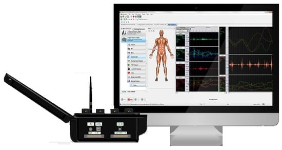
Figure 1.
Trigno wireless electromyography (EMG) acquisition system.
It does not need to pierce the skin of the collector to record the activity of muscle units, but can obtain useful muscle information from the muscle surface. Experiments and data show that the sEMG signal is a very weak bioelectrical signal, with the amplitude of 100–5000 μV, the peak value of 0–6 mV and the root mean square of 0–1.5 mV. The useful signal frequency components of sEMG are in the range of 0–500 Hz, and the main frequency range is in the range of 50–150 Hz [13].
The Trigno sensor was attached to the skin of the volunteers using bioassay tape. It mainly uses four silver bar contacts to collect skin surface EMG signals, as shown in Figure 2. The silver contact electrode has good chemical stability and can reduce the error caused by skin perspiration and air humidity change [14]. There is an arrow with an indicator light on the top of the Trigno sensor to help determine the orientation of the sensor.
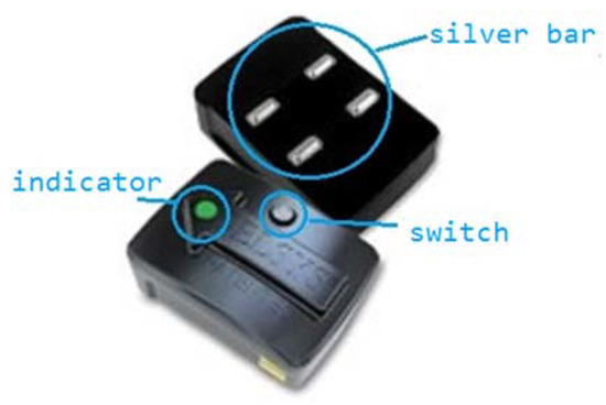
Figure 2.
Trigno sensor.
2.2. Experimental Muscle Selection
Gluteus maximus (GM), vastus medialis (VM), rectus femoris (RF), vastus lateralis (VL), semitendinosus (SE), biceps femoris (BF), tibilis anterior (TA) and gastrocnemius (GA) were selected as sEMG signal [15]. The functions and positions of muscles are shown in Figure 3.
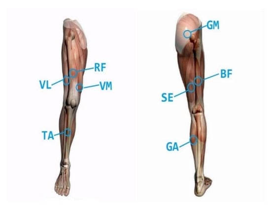
Figure 3.
Description of lower extremity muscle position.
GM starts from the outside of the hip wing and ends at the hip tract. This muscle is controlled by the inferior gluteal nerve. The main function of this muscle is to extend the thigh backward, and to keep the trunk upright and balance when the lower limbs are fixed.
VM is located in the anteromedial part of the femur. It starts from the medial lip of the thick line of the femur and ends at the trochanter of the femur. It forms a muscle tendon flap, which is controlled by the femoral nerve. This muscle function is to realize the knee extension.
RF originates from the inferior iliac spine and ends at the anterior tibial eminence. It is a superficial muscle in the middle of the front thigh and is controlled by the femoral nerve. This muscle has the function of extending the knee joint and bending the thigh.
VL starts from the lateral lip of the femoral thick line and ends at the trochanter of the femur. It is controlled by the femoral nerve. Its main function is to bend the hip joint and extend the knee joint.
SE is one of the posterior thigh muscles, which starts from the ischial tubercle and ends at the medial surface of the upper tibia. It is controlled by the sciatic nerve. It can mainly bend the knee joint and extend the hip joint.
BF originates from the ischial node and ends at the fibular head, which is controlled by the sciatic nerve. BF can bend the knee joint and extend the hip joint. When bending the knee, BF can make crus turn outward.
TA is one of the anterior group muscles of the leg. It starts from the lateral side of the tibia and ends at the plantar surface of the medial cuneiform bone. It is controlled by the deep peroneal nerve. Its main function is to extend the ankle.
GA is located under the skin, starting from the back of the medial and ending at the root bone. It is controlled by the tibial nerve. Its main function is to bend the ankle. When standing, it is responsible for fixing the ankle joint and preventing the body from leaning [16].
The muscle selection of this experiment was determined by analyzing the contribution of muscle to sEMG during joint movement. Twelve healthy participants (6 males and 6 females, 25 ± 2 years old) were asked to perform the following actions. All the participants read and signed an informed consent form approved by the Hangzhou Dianzi University’s Institutional Review Board. The experimental actions are as follows: the participants were seated, (1) the lower limbs of the participants were not moved; (2) the ankle joint was extended and flexed separately; (3) the knee joint was extended and flexed separately; (4) the hip joint was extended and flexed separately. The time duration of each task was 10 s, and the sampling frequency of sEMG is 2000 Hz. According to the contribution of the experimental muscle, the relationship between joint movement and muscle was analyzed. Finally, the most relevant muscle was selected. Muscle contribution was defined as the ratio of the integral value of one muscle sEMG to the sum of the integral values of all muscles in the complete experiment. Then, the contribution of one muscle participating in an action can be defined as:
where a total of k muscles are involved in this action, is the total number of data points of sEMG signals collected by the muscle and is the -th sEMG value of the -th muscle. Table 1 presents the muscle contribution of various movements. Those results are a mean value of several acquisitions from a participant.

Table 1.
Muscle contribution of various movements.
As shown in Table 1, sEMG signals of GM (ch5), RF (ch4), VM (ch3), GA (ch2) and TA (ch1) will be collected as input signals in subsequent experiments. The collected muscles and sensor channels are shown in Figure 4.
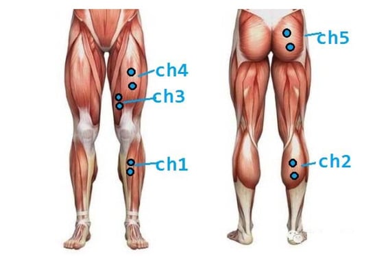
Figure 4.
Sensor acquisition location and direction, ch1 means Channel 1.
2.3. Experimental Action Specification
In this research, we chose the Codamotion system (UK Charnwood Dynamics Ltd.) to capture the real-time motion of our experimental movement and analyze the angle change of the human joint synchronously [17]. The completed experimental platform is shown in Figure 5. We used two channels of Codamotion to collect the real joint angle, and used Trigno to collect sEMG signals synchronously.
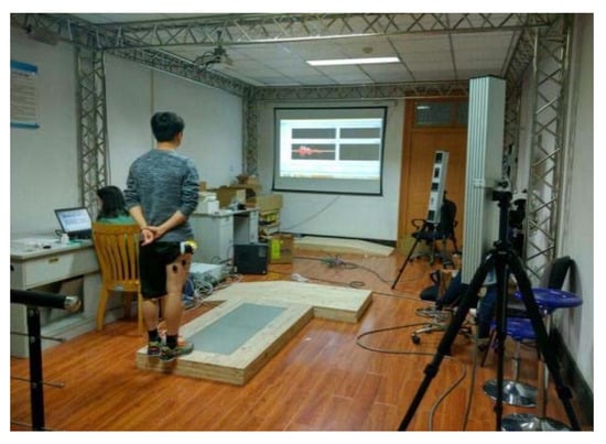
Figure 5.
Experimental platform.
Knee joint stretching and bending is the most commonly used rehabilitation exercise for patients with lower extremity paralysis in the hospital, so we used knee joint stretching and bending exercises as the basis of the first group of experimental actions [18]. The first group of experiments mainly studied the flexion and extension motion of the knee joint and analyzed the flexion and extension motion trend of hip joint and ankle joint. Through the comprehensive analysis of the three joint movements of lower limbs, the sEMG signals could predict the joint angles more accurately and achieve a better rehabilitation effect. Volunteers sat in a chair 60 cm high, with their legs suspended naturally, their hips, knees and ankles relaxed, and then extended and bent their knees periodically. The action breakdown is shown in Figure 6. The knee extension and flexion movements were divided into: (1) fast knee extension and flexion movement, 3 times in 10 s; (2) slow knee extension and flexion movement, 2 times in 10 s. The knee angle is defined as the angle β between the thigh and the lower leg.
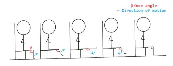
Figure 6.
Knee joint stretching and bending.
Walking and squatting are the most common daily movements of the lower limbs, and the complete rehabilitation training should also include the daily movements. The purpose of this study was also to predict the intention of lower limb joint movement in walking and squatting [19]. The schematic diagram of action decomposition is shown in Figure 7; Figure 8. The angle of the hip joint is defined as the angle between the limb stem and the thigh, the angle of the knee joint is defined as the angle between the thigh and the calf, and the angle of the ankle joint is defined as the angle between the calf and the dorsum of the foot.
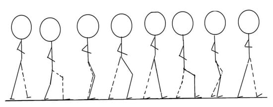
Figure 7.
Walking action decomposition.
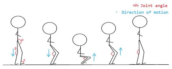
Figure 8.
Squatting action decomposition.
Volunteers stood on the ground naturally—their hips, knees and ankles were in a state of natural relaxation—and then walked and squatted at a regular speed. Walking movement was divided into: (1) fast walking movement, 8 steps within 10 s; (2) slow walking movement, 4 steps within 10 s. The squatting movement was divided into: (3) fast squatting movement, 3 squats in 10 s; (4) slow squatting movement, 2 squats in 10 s.
We selected the muscles identified in Section 2.2 to collect sEMG signals and selected appropriate locations to place Codamotion markers near the hip, knee and ankle joints, as shown in Figure 9.
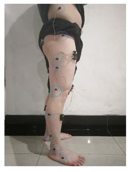
Figure 9.
Codamotion marker placement.
Each volunteer was assigned to do the same experiment. To reduce the collection errors caused by muscle fatigue, we stipulated that each volunteer needed to carry out 5 min of muscle relaxation activities after completing a group of experimental actions [20]. Relaxation activities mainly involved massaging leg muscles. All experimental situations are shown in Table 2.
Table 2.
Six experimental situations and abbreviations.
2.4. Signal Preprocessing
In the data acquisition experiment, we set the sampling frequency of sEMG as 2000 Hz. The acquisition frequency of real-time angle signals was 200 Hz. To unify the signal frequency, we used the average sub-sampling processing method. Although the Trigno system was equipped with a 20–450 Hz bandpass filter, environmental factors still produced a large amount of noise interference. In order to improve the signal-to-noise ratio of the signal, we must conduct secondary denoising for the acquired sEMG signal [21].
Empirical mode decomposition (EMD) is an adaptive time–frequency domain noise reduction method [22]. The EMD algorithm will first decompose the original sEMG signal into a number of intrinsic mode functions (IMF). The IMF mode represents the characteristics of the original sEMG signals at different time scales. Compared with short-time Fourier transform (STFT) and wavelet transform (DWT), the EMD denoising algorithm can deal with non-stationary and nonlinear signals like sEMG better. The EMD algorithm is as follows Algorithm 1:
| Algorithm 1 |
| 1: Initialization , is the original signal, is the number of decomposition layers 2: Get the i-th IMF (1): Initialization , is the extremum function, is the current index (2): Find out the local extremum of (3): Find out the upper and lower envelope of (4): Calculate the average value of the upper and lower envelope lines (5): (6): If is an IMF function, ; Else , transfer to (2) 3: 4: If the number of extremum points is still more than two, , transfer to (2); else, algorithm termination, . |
In this section, the sEMG signals collected in Section 2.2 are used to carry out the noise reduction experiment on the EMD algorithm. sEMG signals of the VM in the knee joint movement were selected for the denoising experiment. The original sEMG signals are shown in Figure 10.
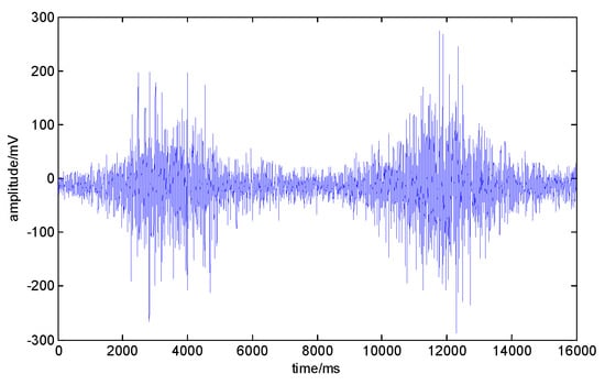
Figure 10.
The original surface electromyography (sEMG) signal of the vastus medialis (VM). The abscissa is the number of signal points, and the ordinate is the signal amplitude.
The EMD algorithm was used to decompose the sEMG signal by 5 layers, and the 5 IMF components obtained by the decomposition were shown in Figure 11.
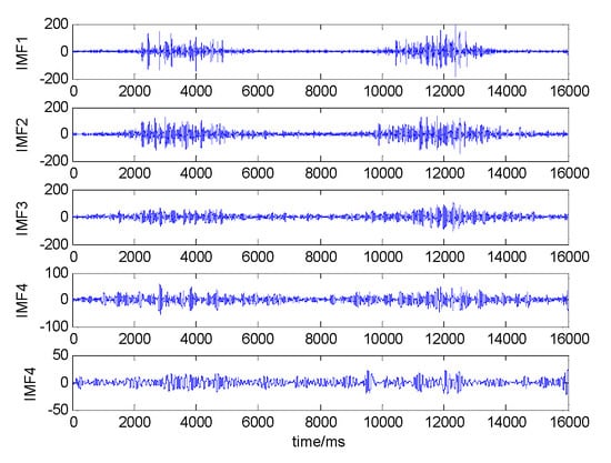
Figure 11.
Five-layer decomposition of sEMG in the VM. The abscissa is the number of signal points, and the ordinate is the signal amplitude
To measure the IMF component obtained by decomposition, we use the Hilbert–Huang Transform (HHT) to carry out the Hilbert transform on the IMF component, as shown in the following formula:
where is instantaneous frequency of the signal, is the analytical amplitude of the j-th IMF component, is frequency function, is the total is the number of decomposition layers.
By expanding the real part after the transformation of the above formula, we can get the Hilbert spectrum, as following:
The marginal spectrum can be obtained by integrating the time dimension of the Hibert spectrum, as shown in the following formula:
The Hilbert marginal spectrum is the integral of the sEMG signal in the time dimension. The marginal spectrum amplitude can reflect whether a certain frequency really exists in the sEMG signal. Since sEMG signal frequency is mainly distributed between 0 and 500 Hz, the instantaneous frequency of sEMG can be obtained by the HHT transformation above. In noise reduction experiments, the effectiveness is defined to measure the effectiveness of each component. In the experiment, the is defined to measure the effectiveness of each component. We believe the IMF weight is effective when where is the effective frequency points in the i-th IMF component, and is the total number of points of the IMF. The effectiveness of each IMF component is shown in Table 3.
Table 3.
Intrinsic mode functions (IMF) component validity.
It can be seen from Table 3 that the IMF components of the first three layers are effective, so the sEMG signal can be reconstructed from the IMF components of these three layers. The comparison between the original signal and the denoised signal in this noise reduction experiment is shown in Figure 12.
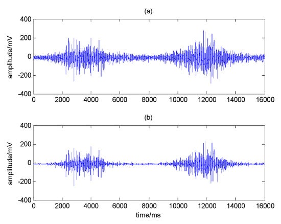
Figure 12.
Comparison diagram of (a) original signal and (b) denoised signal.
2.5. sEMG Feature Extraction Based on Wavelet Packet
First, we introduce two time domain features and one frequency domain feature defined as follows:
1. Integrated EMG (IEMG)
IEMG is usually used as a performance index of EMG pattern recognition and clinical application. IEMG features are defined as the sum of absolute values of EMG signal amplitude [23], which can be expressed as:
where is the amplitude of EMG at time and is the length of the sEMG sequence.
2. Root mean square (RMS)
RMS is another popular feature in sEMG analysis. It is considered as a Gaussian stochastic process [24]. The mathematical definition of RMS features can be expressed as:
3. Mean power (MNP)
MNP is the average power of sEMG power spectrum [25]. The calculation is defined as:
where is the sEMG power spectrum at frequency , and is the length of the frequency signal.
Due to the non-stationary characteristics of sEMG signal, short-time Fourier transform (STFT), wavelet transform (WT) and other time–frequency analysis methods are more suitable for processing sEMG signal. In recent years, the time–frequency analysis method has been favored more by the majority of scholars [26].
The wavelet packet analysis divides the time and frequency plane more carefully, as shown in Figure 13, and the resolution of the high-frequency part of the signal is higher than that of the binary wavelet. Furthermore, it introduces the concept of optimal basis selection on the basis of the wavelet analysis theory. In other words, after dividing the frequency band into several layers, according to the characteristics of the signal being analyzed, the optimal basis function is selected adaptively to match with the signal, so as to improve the analysis ability of the signal [27].
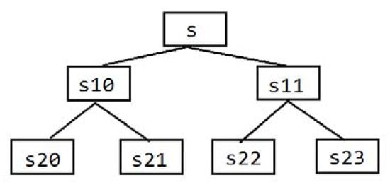
Figure 13.
Wavelet packet decomposition. S is the original signal, s10 is the first signal of Layer 1 decomposition and s20 is the first signal of Layer 2 decomposition.
We first extract the coefficients of each layer , where is the number of decomposition layers of the current wavelet packet, and is the index of the current wavelet coefficient. Then, we compute the time domain and frequency domain characteristics of all the . In this way, we can obtain the combined features: wavelet packet–root mean square (WP–RMS), wavelet packet–root mean square (WP–RMS) and wavelet packet–mean power (WP–MNP). In the prediction experiments, we will use combined features as input vectors.
2.6. Construction of ELM Prediction Network
ELM was proposed by professor Huang of Nanyang Technological University [28]. It is a kind of machine learning method based on the Feedforward Neuron Network (FNN), which can be used to solve supervised and unsupervised learning problems. ELM is considered to be a special type of FNN, or an improvement of Back Propagation (BP) algorithms. Its characteristic is that the weight of the hidden layer node can be a randomly determined value or an artificial given value, and it does not need to be updated. The learning process only needs to calculate the output weight. According to the characteristics of sEMG data, we found that the training effect of ELM was better than BP [29].
ELM is a single hidden layer structure like the traditional FNN, and its structure topology is shown in Figure 14. Compared with other shallow learning systems such as the single-layer perceptron and support vector machine, ELM is faster than the traditional learning algorithm on the premise of ensuring learning accuracy. sEMG signals are irregular and nonstationary, using the ELM prediction model to process such data can make the training speed faster.
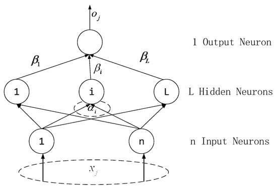
Figure 14.
Single hidden layer extreme learning machine (ELM) structure.
For ELMs with a single hidden layer, there are arbitrary samples , where ,. For a single hidden layer neural network with hidden layer nodes, it can be expressed as:
where is the activation function of the output layer, is the input weight, is the output weight, and is the offset of the i-th hidden layer unit. is the inner product of and .
The goal of weight learning of a single hidden layer neural network is to minimize the output error, which can be expressed as follows:
There are , and :
It can also be expressed as:
where is the output of the hidden layer node, is the output weight, and is the expected output.
In order to train single hidden layer neural networks, we need to find , and :
This is equivalent to the existence of a minimum loss function:
The traditional BP algorithm can be used to solve the above problems, but the traditional algorithm may calculate and modify all network parameters, which has a large amount of calculation and slow training speed. In the ELM algorithm, once the input weight and the offset of the hidden layer are determined as a random value, the output matrix is uniquely determined [30]. Then, the above problem can be transformed into solving a linear system, and the output weight is uniquely determined:
where is the Moore Penrose Inverse of matrix , and it can be proved that the norm of the solution is the smallest and the only.
All the experimental data were collected from 12 healthy volunteers. The volunteers performed the experimental actions according to the 6 situations defined in Section 2.3. Each volunteer did 10 groups of actions under different conditions. For each experimental situation, we can get 120 samples. In this study, we used the following root mean square error (RMSE) indicators to evaluate the prediction performance of the prediction model. The smaller the evaluation index value, the better the prediction effect of the model. The calculation formula is as follows:
where is the total number of samples, is the real angle value, and is the predicted angle value.
All the prediction results were processed by the method of six-fold cross-validation. The samples of each experimental action 120 were randomly divided into six equal groups, one of which was used as test data, the other five as training data. We repeated this operation for each set of data, so we could get six results [31], and RMSE in the following prediction results is the average of these six results.
In order to determine the structure of ELM in the experiment, we first determined the hidden layer node as 15 according to the estimation of Formula (16), and set the hidden layer transfer function as sigmoid function [32].
Among them, is the number of neurons in the hidden layer, is the number of neurons in the input layer, is the number of neurons in the output layer, and is a constant between 1 and 10. Then, we chose 5, 10, 15, 20 and 25 as hidden layer nodes and built a prediction model for each hidden layer node. Finally, we used the verification set of each action to verify the prediction performance of the prediction model. Among the five models, we chose the model with the least RMSE in the verification experiment, and thought that it can predict the experimental results well. After the comparison experiment on the number of hidden layer nodes, we can see from Figure 15 shows that in the ELM prediction model, choosing the number of hidden layer nodes as 10 can get the best prediction result.
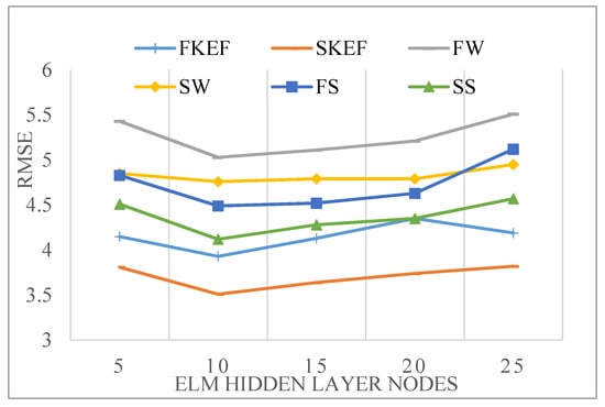
Figure 15.
RMSE of prediction results when the number of ELM neurons changes.
3. Results
3.1. Analysis of Joint Angle Prediction Results
In the characteristic performance comparison experiment, we use IEMG, RMS and MNP to extract the features. Then, we can obtain the combined features WP–IEMG, WP–RMS and WP–MNP.
We selected fast knee extension and flexion (FKEF) and slow knee extension and flexion (SKEF) data as input data, and trained the ELM model to predict hip, knee and ankle angles for each feature. The RMSE is shown in Table 4, and the experimental results of using WP–RMS characteristics are shown in Figure 16.
Table 4.
RMSE with different input features.
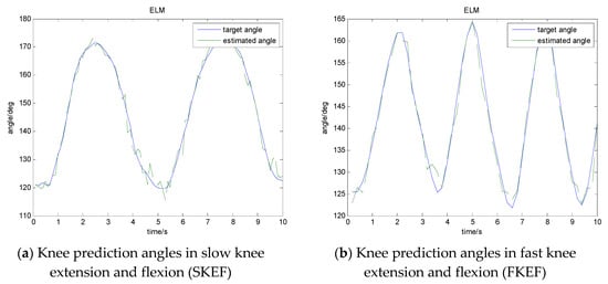
Figure 16.
Prediction results of knee extension and flexion.
RMSE in Table 4 and Figure 16 is the average value of our experimental results. In most of the experimental results, the RMSE value of slow knee extension and flexion is smaller than that of fast knee extension and flexion. We can see that the prediction error RMSE increases with the increase of knee extension and flexion speed, and the prediction error RMSE obtained when WP–RMS feature is used as the input feature set is obviously better than other sEMG feature extraction methods. We also used the WP–RMS feature training ELM to study the prediction results of each movement of different volunteers. The RMSE values of all volunteers are shown in Figure 17. In all conditions, the same volunteers had greater predictive errors in FW. In the same condition, the difference in prediction error between the volunteers was not significant. The results show that our method can achieve good prediction performance for each volunteer. Fast walking is more complex and involves more muscles. The joint angles collected in the experiment are the vector angle on the vertical plane, and the actual joint angles of walking are three-dimensional, so fast walking has a greater RMSE value than fast knee extension and flexion.
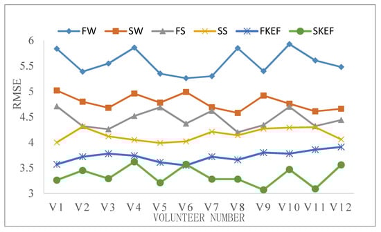
Figure 17.
RMSE for each experimental condition of different volunteers.
3.2. Correlation Analysis of sEMG Signals and Joint Angles Based on DCCA
DCCA was proposed in 1994 by Peng and is used to analyze the time series of the long-range correlation method [11]. The DCCA method can filter out the trend components in the original time series perfectly and avoid noise interference to analyze the correlation of a polynomial trend signal. This algorithm is especially suitable for analyzing the correlation of non-stationary time series such as sEMG, which fully meets the requirements of sEMG analysis. The main flow of the algorithm is as follows Algorithm 2:
| Algorithm 2 |
| 1: Given two time series and with length , the sum sequence of the two series are calculated as and . 2: The whole sequence is divided into groups, each with time series. 3: The least square method was used to fit each group and calculate the local trend . 4: Calculate the residual covariance for each group, . 5: Finally, the sum of the overlapping groups give the detrended covariance, |
The DCCA algorithm is used to quantitatively analyze the mutual correlation between two non-stationary time series, and has no special requirements on time series. Even though the original time series was originally doped with noise, the correct analysis can still be obtained [33]. If the two time series are mutually correlated, then the trend error follows the curtain law distribution , where is the cross-correlation index and is the similarity parameter.
We selected the data of the slow squat experiment, then analyzed the sEMG data of the same length and the prediction angle data, and obtained the distribution of the detrended fluctuation analysis (DFA) index of the two signals and the DCCA index of each other, as shown in Table 5 and Figure 18.
Table 5.
Detrended cross-correlation analysis (DCCA) index between predictive angles and sEMG signals.
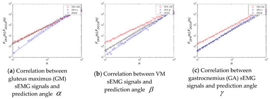
Figure 18.
Detrended fluctuation analysis (DFA) and DCCA index of sEMG signals and prediction angles.
Table 5 shows the statistical results of the DCCA mean value of all muscle signals and joint angle signals under the slow squat movement. It is found that the DCCA mean value of the correlation number increases gradually with the increase of the closeness between muscle and joint. As can be seen from Figure 18a–c, for the three different joints of the hip, knee and ankle, the sEMG signals of each muscle and the prediction angle value of DCCA are different. Only by finding the most relevant muscles of the joint and increasing the proportion of the muscle sEMG in the extracted features can the joint angle signals be better predicted. By improving the feature extraction algorithm of WP–RMS, we can change the layers of wavelet packet decomposition of the sEMG signal in different channels to match each different joint to achieve a better prediction effect.
4. Discussion and Conclusions
Aiming at the accuracy and rapidity of prediction, a method of multi-joint angle continuous motion prediction based on sEMG is proposed. We collected the sEMG signals of five muscle groups of human lower limbs. The EMD decomposition algorithm was used to reduce the noise of the sEMG signal. A feature extraction method based on the wavelet packet as was proposed for the EMG signal. The ELM prediction model was constructed to train the feature data. The experimental results of different volunteers were analyzed, which show the effectiveness of the method. Finally, the correlation between the EMG signal and the prediction angle signal was analyzed, which provides support for improving the prediction model.
This research mainly collected the experimental data for multi-joint continuous motion prediction by using the Trigno and Codamotion systems, which provide the possibility for improving the accuracy of multi-joint continuous prediction, and technical support for applying the research results of multi-joint continuous prediction to rehabilitation training, intelligent robot and other fields. However, there are still the following deficiencies in this study:
1. The purpose of this study was mainly to predict the angles of lower limb joints based on sEMG signals, so that the rehabilitation robot can have a better training effect. Patients in need of rehabilitation training are generally the elderly or people with mobility disorders, but this study only invited healthy young volunteers in the laboratory. sEMG signals between the two are similar in the transformation trend, but there is a difference in amplitude. The amplitude of sEMG signals in patients is weaker than that in healthy people, so we need to consider how to enhance patients’ sEMG signals to make the predicted results meet expectations.
2. In this paper, the main experimental methods are offline data collection, training network model and joint angle prediction. For the actual rehabilitation training scenario, we need to determine the time efficiency of prediction model training and prediction in the online environment. On the other hand, the volunteers in this study mainly experimented with three movements: knee extension and flexion, walking and squatting. In the follow-up study, we need to add more experiments covering more rehabilitation training actions, and increase the complexity of the experimental environment to adapt to the actual rehabilitation training scene.
Author Contributions
J.W. and L.W. conceived and designed the research and wrote the manuscript; J.W. and X.X. performed the research; S.M.M. and A.X. wrote and reviewed the manuscript. All authors have read and agreed to the published version of the manuscript.
Funding
This work was supported by the National Natural Science Foundation of China (Nos. 61971169 and 60903084) and National Natural Science Major Foundation of Research Instrumentation of China under Grant 61427808.
Conflicts of Interest
The authors declare no conflicts of interest.
References
- Go, A.S.; Mozaffarian, D.; Roger, V.L.; Benjamin, E.J.; Berry, J.D.; Borden, W.B.; Bravata, D.M.; Dai, S.; Ford, E.S.; Fox, C.S.; et al. Executive Summary: Heart Disease and Stroke Statistics--2013 Update: A Report From the American Heart Association. Circulation 2013, 127, 143–152. [Google Scholar] [CrossRef]
- Howell, M.; Gottschall, P.E. Lectican proteoglycans, their cleaving metalloproteinases, and plasticity in the central nervous system extracellular microenvironment. Neuroscience 2012, 217, 6–18. [Google Scholar] [CrossRef]
- Buchanan, T.; Lloyd, D.; Manal, K.; Besier, T. Neuromusculoskeletal Modeling: Estimation of Muscle Forces and Joint Moments and Movements from Measurements of Neural Command. J. Appl. Biomech. 2004, 20, 367–395. [Google Scholar] [CrossRef]
- Han, J.; Ding, Q.; Xiong, A.; Zhao, X. A State-Space EMG Model for the Estimation of Continuous Joint Movements. IEEE Trans. Ind. Electron. 2015, 62, 4267–4275. [Google Scholar] [CrossRef]
- Favre, J.; Hayoz, M.; Erhart-Hledik, J.; Andriacchi, T.P. A neural network model to predict knee adduction moment during walking based on ground reaction force and anthropometric measurements. J. Biomech. 2012, 45, 692–698. [Google Scholar] [CrossRef]
- Jiang, N.; Vujaklija, I.; Rehbaum, H.; Graimann, B.; Farina, D. Is Accurate Mapping of EMG Signals on Kinematics Needed for Precise Online Myoelectric Control? IEEE Trans. Neural Syst. Rehabilitation Eng. 2013, 22, 549–558. [Google Scholar] [CrossRef]
- Yu, H.-J.; Lee, A.; Choi, Y. Human elbow joint angle estimation using electromyogram signal processing. IET Signal Process. 2011, 5, 767–775. [Google Scholar] [CrossRef]
- Cheron, G.; Leurs, F.; Bengoetxea, A.; Draye, J.P.; Destrée, M.; Dan, B. A dynamic recurrent neural network for multiple muscles electromyographic mapping to elevation angles of the lower limb in human locomotion. J. Neurosci. Methods 2003, 129, 95–104. [Google Scholar] [CrossRef]
- Zhang, F.; Li, P.; Hou, Z.-G.; Lu, Z.; Chen, Y.; Li, Q.; Tan, M. sEMG-based continuous estimation of joint angles of human legs by using BP neural network. Neurocomputing 2012, 78, 139–148. [Google Scholar] [CrossRef]
- Chen, J.; Zhang, X.; Cheng, Y.; Xi, N. Surface EMG based continuous estimation of human lower limb joint angles by using deep belief networks. Biomed. Signal Process. Control. 2018, 40, 335–342. [Google Scholar] [CrossRef]
- Podobnik, B.; Stanley, H.E. Detrended Cross-Correlation Analysis: A New Method for Analyzing Two Nonstationary Time Series. Phys. Rev. Lett. 2008, 100, 084102. [Google Scholar] [CrossRef]
- Chen, X.; Wang, Z.J. Pattern recognition of number gestures based on a wireless surface EMG system. Biomed. Signal Process. Control. 2013, 8, 184–192. [Google Scholar] [CrossRef]
- Xi, X.; Tang, M.; Miran, S.M.; Luo, Z. Evaluation of Feature Extraction and Recognition for Activity Monitoring and Fall Detection Based on Wearable sEMG Sensors. Sensors 2017, 17, 1229. [Google Scholar] [CrossRef]
- Tenore, F.; Ramos-Murguialday, A.; Fahmy, A.; Acharya, S.; Etienne-Cummings, R.; Thakor, N.V. Decoding of Individuated Finger Movements Using Surface Electromyography. IEEE Trans. Biomed. Eng. 2009, 56, 1427–1434. [Google Scholar] [CrossRef]
- Hermens, H.J.; Freriks, B.; Disselhorst-Klug, C.; Rau, G. Development of recommendations for SEMG sensors and sensor placement procedures. J. Electromyogr. Kinesiol. 2000, 10, 361–374. [Google Scholar] [CrossRef]
- Fridlund, A.J.; Cacioppo, J.T. Guidelines for Human Electromyographic Research. Psychophysiology 1986, 23, 567–589. [Google Scholar] [CrossRef]
- Monaghan, K.; Delahunt, E.; Caulfield, B. Increasing the number of gait trial recordings maximises intra-rater reliability of the CODA motion analysis system. Gait Posture 2007, 25, 303–315. [Google Scholar] [CrossRef]
- Liu, S.-C.; Hou, Z.-L.; Tang, Q.-X.; Qiao, X.-F.; Yang, J.-H.; Ji, Q.-H. Effect of knee joint function training on joint functional rehabilitation after knee replacement. Medicine 2018, 97, e11270. [Google Scholar] [CrossRef]
- Sartori, M.; Reggiani, M.; Farina, D.; Lloyd, D.G. EMG-Driven Forward-Dynamic Estimation of Muscle Force and Joint Moment about Multiple Degrees of Freedom in the Human Lower Extremity. PLoS ONE 2012, 7, 52618–52630. [Google Scholar] [CrossRef]
- Aung, Y.M.; Al-Jumaily, A. sEMG Based ANN for Shoulder Angle Prediction. Procedia Eng. 2012, 41, 1009–1015. [Google Scholar] [CrossRef]
- Li, Y.; Xu, M.; Wei, Y.; Huang, W. An improvement EMD method based on the optimized rational Hermite interpolation approach and its application to gear fault diagnosis. Measurement 2015, 63, 330–345. [Google Scholar] [CrossRef]
- Zheng, J.; Cheng, J.; Yang, Y. Generalized empirical mode decomposition and its applications to rolling element bearing fault diagnosis. Mech. Syst. Signal Process. 2013, 40, 136–153. [Google Scholar] [CrossRef]
- Huang, H.-P.; Chen, C.-Y. Development of a myoelectric discrimination system for a multi-degree prosthetic hand. In Proceedings of the 1999 IEEE International Conference on Robotics and Automation, Detroit, MI, USA, 10–15 May 1999; pp. 2392–2397. [Google Scholar]
- Du, S.; Vuskovic, M. Temporal vs. spectral approach to feature extraction from prehensile EMG signals. In Proceedings of the 2004 IEEE International Conference on Information Reuse and Integration, Las Vegas, NV, USA, 8–10 November 2005; pp. 344–350. [Google Scholar]
- Hudgins, B.; Parker, P.; Scott, R. A new strategy for multifunction myoelectric control. IEEE Trans. Biomed. Eng. 1993, 40, 82–94. [Google Scholar] [CrossRef]
- Boostani, R.; Moradi, M.H. Evaluation of the forearm EMG signal features for the control of a prosthetic hand. Physiol. Meas. 2003, 24, 309–319. [Google Scholar] [CrossRef]
- Xie, H.; Wang, Z. Mean frequency derived via Hilbert-Huang transform with application to fatigue EMG signal analysis. Comput. Methods Programs Biomed. 2006, 82, 114–120. [Google Scholar] [CrossRef]
- Huang, G.-B.; Zhou, H.; Ding, X.; Zhang, R. Extreme Learning Machine for Regression and Multiclass Classification. IEEE Trans. Syst. Man, Cybern. Part B (Cybern.) 2011, 42, 513–529. [Google Scholar] [CrossRef]
- Yang, Z.; Baraldi, P.; Zio, E. A comparison between extreme learning machine and artificial neural network for remaining useful life prediction. In Proceedings of the 2016 Prognostics and System Health Management Conference (PHM-Chengdu), Chengdu, China, 19–21 October 2016; pp. 2166–5656. [Google Scholar]
- Huang, G.-B.; Zhu, Q.-Y.; Siew, C.-K. Extreme learning machine: A new learning scheme of feedforward neural networks. In Proceedings of the 2004 IEEE International Joint Conference on Neural Networks (IEEE Cat. No.04CH37541), Budapest, Hungary, 25–29 July 2004; pp. 985–990. [Google Scholar]
- Shao, Z.; Er, M.J.; Wang, N. An Efficient Leave-One-Out Cross-Validation-Based Extreme Learning Machine (ELOO-ELM) With Minimal User Intervention. IEEE Trans. Cybern. 2015, 46, 1939–1951. [Google Scholar] [CrossRef]
- Yuan, H.; Xiong, F.; Huai, X. A method for estimating the number of hidden neurons in feed-forward neural networks based on information entropy. Comput. Electron. Agric. 2003, 40, 57–64. [Google Scholar] [CrossRef]
- Wang, J.; Zhao, D.-Q. Detrended cross-correlation analysis of electroencephalogram. Chin. Phys. B 2012, 21, 28703. [Google Scholar] [CrossRef]


© 2020 by the authors. Licensee MDPI, Basel, Switzerland. This article is an open access article distributed under the terms and conditions of the Creative Commons Attribution (CC BY) license (http://creativecommons.org/licenses/by/4.0/).