A Multi-Switching Tracking Control Scheme for Autonomous Mobile Robot in Unknown Obstacle Environments

Abstract

The obstacle avoidance control of mobile robots has been widely investigated for numerous practical applications. In this study, a control scheme is presented to deal with the problem of trajectory tracking while considering obstacle avoidance. The control scheme is simplified into two controllers. First, an existing trajectory tracking controller is used to track. Next, to avoid the possible obstacles in the environment, an obstacle avoidance controller, which is used to determine the fastest collision avoidance direction to follow the boundary of the obstacle at a constant distance, is proposed based on vector relationships between the robot and an obstacle. Two controllers combined via a switch strategy are switched to perform the task of trajectory tracking or obstacle avoidance. The stability of each controller in the control scheme is guaranteed by a Lyapunov function. Finally, several simulations are conducted to evaluate the proposed control scheme. The simulation results indicate that the proposed scheme can be applied to the mobile robot to ensure its safe movement in unknown obstacle environments.

1. Introduction

In recent years, the wheeled mobile robot (WMR) has received much attention due to its many practical applications, which is widely used in various aspects, such as search and rescue [1], multi-robotic formation [2,3], industrial applications [4,5], military operations [6,7], and so on. These applications require the mobile robot to move autonomously and carry out a variety of automated tasks which include trajectory tracking, obstacle avoidance, formation control, etc. For the control of mobile robots, the major challenge is to develop effective controllers to deal with various tasks. Among those tasks, the problems of obstacle avoidance and trajectory tracking are especially important for autonomous movement.

Obstacle avoidance is a necessary function in robotics technology. It aims to ensure the robot would not collide with obstacles in unknown environments. The obstacle avoidance problem has been investigated by many researchers. In [8], a path planning algorithm was designed using the sensor fusion of a camera and a laser radar to generate a collision-free path. In addition, artificial potential field (APF) [9,10] methods were presented for obstacle avoidance. They use a potential field function to generate an obstacle-free trajectory by creating an attractive force for the goal and a repulsive force around the obstacle to avoid collision. In [11,12], The genetic algorithms (GA) inspired by evolutionary theory were devised to generate optimal paths from one start point to the target location within given obstacles. In [13], A hybrid approach combined APF and GA was presented to find a feasible path for the multi-objective path planning problem. In [14,15], some common optimization technologies like particle swarm optimization (PSO) and ant colony optimization (ACO) were also presented to resolve the obstacle avoidance problem in terms of multi-objective optimization. However, the main drawbacks of those heuristic or evolutionary methods based on optimization techniques are that they have possible local minimum problem in computation, and their computations are complicated. In order to solve those limitations, researchers studied the obstacle avoidance problem based on control theory, and obstacle avoidance methods using the geometric relationship between the robot and an obstacle were proposed to avoid possible obstacle [16,17,18,19]. Whereas the above-mentioned works only consider obstacle avoidance for mobile robots without taking trajectory tracking into account.

Robots follow a desired trajectory generated by a virtual mobile robot based on its kinematic model and initial posture, which can navigate the mobile robot to the desired position. This tracking problem has been studied by many researchers, and there are a lot of control strategies are proposed for mobile robots, such as model predict control (MPC) [20,21,22], sliding mode control (SMC) [23,24,25,26], fuzzy control [27,28,29], adaptive control [30,31,32], and intelligent control [33,34], etc. However, most of them studied the trajectory tracking problem under the assumption that the movement of the robot is in an obstacle-free environment. Hence, the design of the controller lacks the consideration of the possible collisions in the environment.

In the above discussion, the obstacle avoidance problem is addressed by pathing planning algorithm or obstacle avoidance controller. Besides those mentioned literatures, some studies presented some unified controllers by considering the obstacle avoidance function in trajectory tracking controller to handle the problems of tracking and obstacle avoidance over the past few years [35,36,37,38], few studies have focused on the combination of multiple controllers [39]. Furthermore, it is extremely hard to address the problem of trajectory tracking with obstacles utilizing only one controller for the difficulties in design and the high computational cost. Therefore, the combination of practical, low-computational cost, and effective controllers is important to ensure the movement of the mobile robot.

This paper presents a control scheme for a mobile robot to navigate it from a start position to a desired destination. The mobile robot tracks a pre-planned trajectory by using the reference posture and reference velocities as input signals for its control system. Owing to unknown obstacles in the environment, an obstacle avoidance controller is presented to escape the obstacle. In this paper, the problem of trajectory tracking in unknown obstacle environments is simplified by dividing the objective of control scheme into two controllers, trajectory tracking and obstacle avoidance controllers. Both controllers are designed separately based on their own error dynamic model to execute the corresponding task. In this control scheme, a switch strategy is introduced to combine two controllers, and the current controller executed by the control system of mobile robot is switched between the trajectory tracking controller and the obstacle avoidance controller, which means that only one controller works at specific condition to guarantee the performance of each task In this paper, an existing trajectory tracking controller is used to track the pre-planned trajectory. Once an obstacle is detected by the mobile robot, the safe boundary and risk area of the obstacle are generated by the obstacle controller. When the obstacle avoidance condition is satisfied, a blending vector used to determine the fastest obstacle avoidance direction and follow the boundary of the obstacle to avoid the obstacle. After the completion of the obstacle avoidance, the trajectory tracking controller is activated to track the pre-planned trajectory. The advantage of this control scheme is to divide the complex tracking problem into two simple and low-computational controllers combined via a switch strategy. The stability of the proposed control scheme is proved by a Lyapunov function. In addition, the effectiveness of the proposed control scheme is evaluated by the simulation results.

The rest of this paper is organized as follows. In Section 2, the problem statement related to control scheme is stated. In Section 3, an obstacle avoidance control method is presented to avoid the possible collision. In Section 4, a switch strategy used to combine the tracking and obstacle avoidance controllers is introduced. In Section 5, several simulations are given to validate the effectiveness of the proposed control scheme. In Section 6, brief conclusions and future studies are discussed.

2. Problem Statement

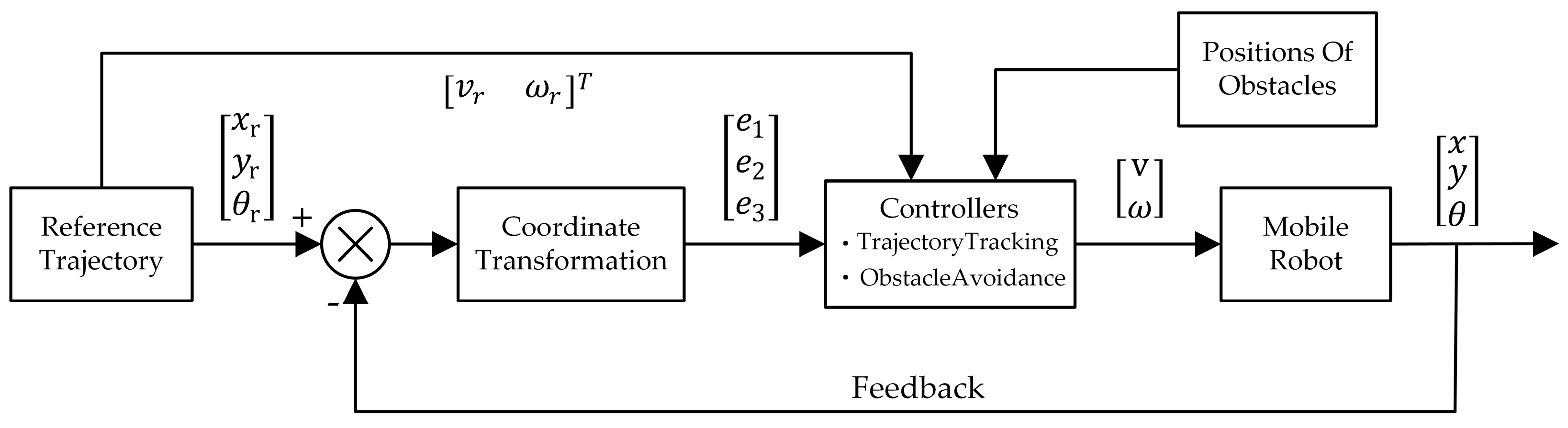
The robot discussed in this paper is a two-wheeled mobile robot. The kinematic model of the robot is described in detailed in [40,41]. The environment where the mobile robot works is always filled with unknown obstacles. That is, static obstacles or dynamic obstacles, and their position information is prior or measured by the sensors attached to the mobile robot during its movement. In this paper, the obstacle avoidance problem can be defined as designing a feasible path from the perspective of control theory, meaning that will not collide with the obstacles. In the control domain of the mobile robot, the task of the mobile robot requires navigating the robot from a start point to a desired position. Trajectory tracking typically plays an important role in the navigation task. In order to implement the trajectory tracking, we use a classic nonlinear control rule to track the trajectory, and then combined with our proposed obstacle avoidance method. In this paper, to deal with the problem that the mobile robot encounters an obstacle when tracking, an obstacle avoidance controller is presented. The basic idea of the controller is to drive the mobile robot to a direction determined by a blending vector to follow the boundary of the obstacle at a constant distance, and then escape the obstacle to track the trajectory.

3. Methodology

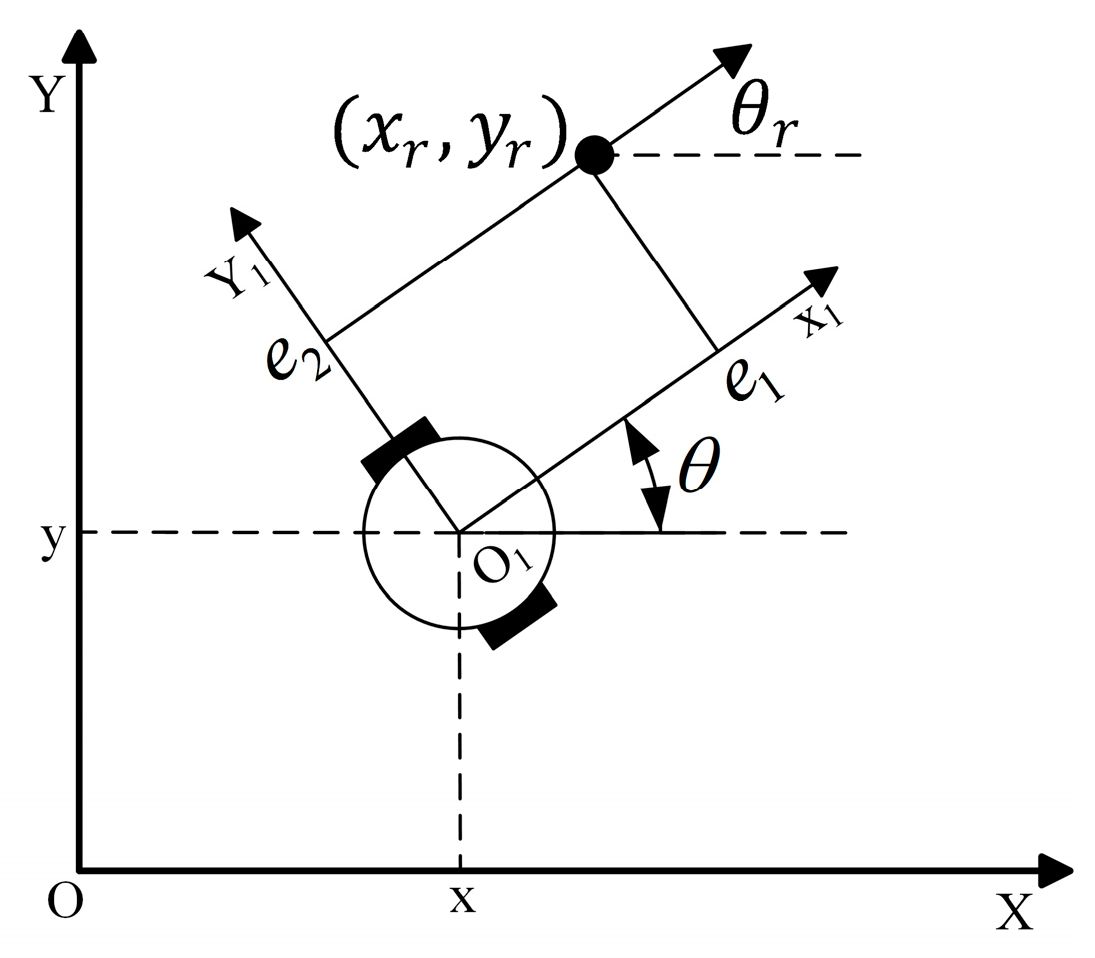
3.1. Trajectory Tracking Control

In this section, an existing trajectory tracking controller is introduced, which aims to find appropriate control inputs of the mobile robot and then make tracking errors to zero when the tracking time goes to infinite.

The trajectory tracking problem that the mobile robot tracks the reference trajectory generated by a moving virtual mobile robot is depicted in Figure 1. Let $q_r={\left[\begin{array}{ccc}{x}_r& y_r& {\theta }_r\end{array}\right]}^T$ denote the posture of the virtual mobile robot, and the current posture of the mobile robot is expressed as $q={\left[\begin{array}{ccc}x& y& \theta \end{array}\right]}^T$. The tracking errors $e_1$, $e_2,$ and $e_3$ between the mobile robot and the virtual mobile robot denoted in the body coordinate system $\left\{O_1\right\}$ are given by

$$\left[\begin{array}{c}{e}_1\\ e_2\\ e_3\end{array}\right]=\left[\begin{array}{cc}\cos \theta & \begin{array}{cc}\sin \theta & 0\end{array}\\ \begin{array}{c}-\sin \theta \\ 0\end{array}& \begin{array}{cc}\begin{array}{c}\cos \theta \\ 0\end{array}& \begin{array}{c}0\\ 1\end{array}\end{array}\end{array}\right]\left[\begin{array}{c}{x}_r-x\\ \begin{array}{c}{y}_r-y\\ {\theta }_r-\theta \end{array}\end{array}\right]$$

(1)

A classic control rule for the trajectory tracking is given [42]

$$v=v_r\cos e_3+k_1{e}_1$$

(2)

$$\omega ={\omega }_r+k_2{v}_r{e}_2+k_3{v}_r\sin e_3$$

(3)

where $k_1$, $k_2,$ and $k_3$ are positive constants. the control inputs described in Equations (2) and (3) are used, the tracking errors $e_1$, $e_2,$ and $e_3$ will converge to zero.

3.2. Obstacle Avoidance Control

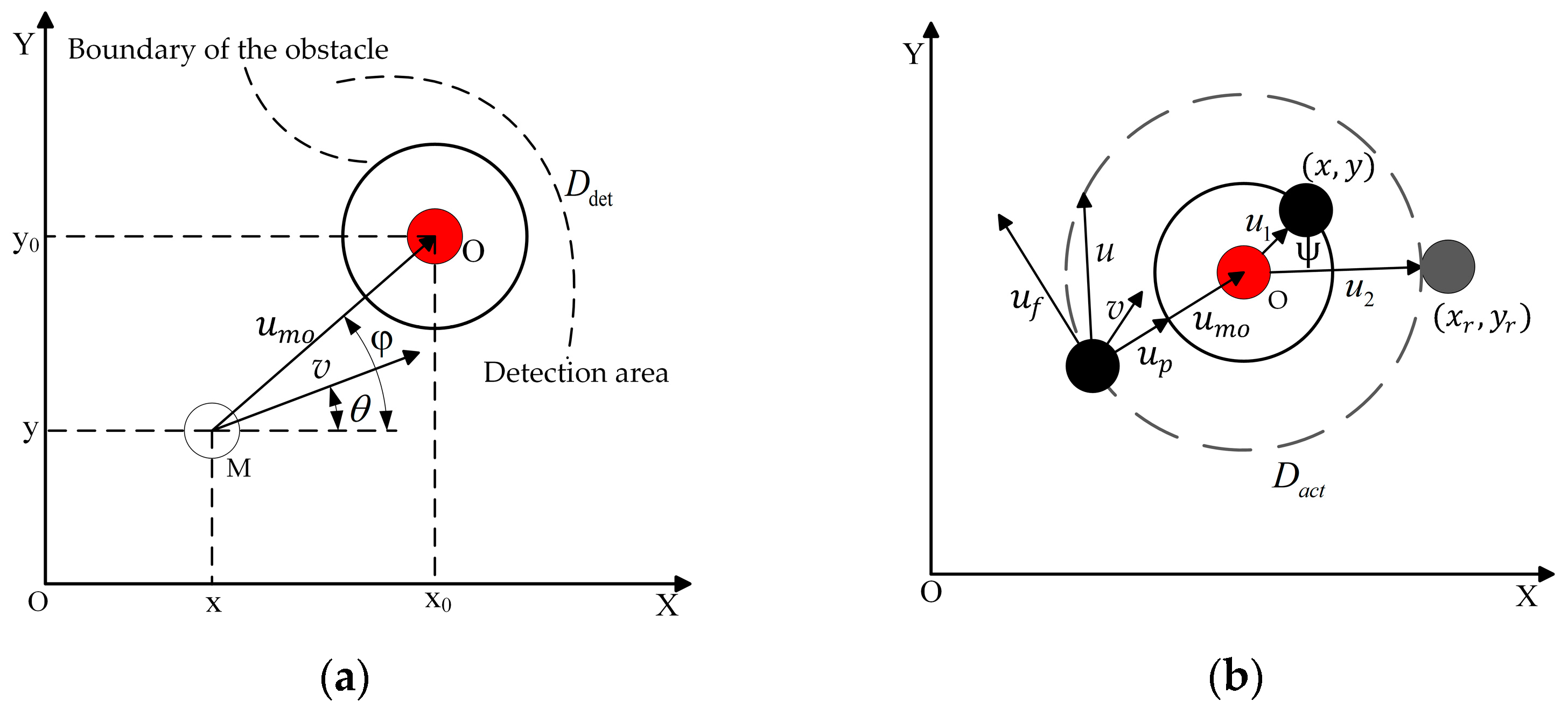
3.2.1. Analysis of Obstacle Avoidance Problem

In this section, a mobile robot is considered with the mission of avoiding collision between the robot and circular obstacles in a two-dimensional plane. Let $M\left(\mathrm{x},\mathrm{y}\right)$ and $O\left(x_0,y_0\right)$ be the positions of the robot and the obstacle, respectively. In order to facilitate the design and analysis of the obstacle avoidance controller, several definitions are introduced in the following.

Definition 1.

An obstacle can be considered be detected by the mobile robot if the following expression is satisfied:

$$D_r\le D_{det}$$

(4)

where$D_{det}$represents the maximum measurement distance of the range sensor attached to the mobile robot.$D_r$denotes the relative distance between the robot and an obstacle, and the$D_r$is calculated by the expression

$$D_r=\Vert {\mathit{u}}_{\mathit{m}\mathit{o}}\Vert =\sqrt{\left(x_0-x\right)+\left(y_0-y\right)}$$

(5)

where

$${\mathit{u}}_{\mathit{m}\mathit{o}}=\left[\begin{array}{c}{x}_0-x\\ y_0-y\end{array}\right]$$

represents a vector pointing from the position of the mobile robot to the position of the obstacle, and$\Vert ·\Vert$represents the Euclidean norm of a vector.

Definition 2.

In practical situations, to avoid the possible collision occurred when the mobile robot tracks the trajectory, a safe distance relative to the obstacle surface is required to be defined to form the safe boundary of the obstacle, which can be denoted as

$$D_s\ge R_m$$

(6)

where$D_s$denotes a constant safe distance from the obstacle, and$R_m$represents the radius of the mobile robot.

Definition 3.

The collision occurs if the relative distance and the safe distance satisfy the following relationship

$$D_r<R_m$$

(7)

Definition 4.

The robot would collide an obstacle if it is going on tracking the reference trajectory, in this case, the robot needs to perform an obstacle avoidance controller to avoid collision when the relative distance$D_r$satisfies the condition

$$D_s<D_r\le D_{act}$$

(8)

where$D_{act}$denotes a distance value to activate the obstacle avoidance controller under the condition that the obstacle avoidance is not completed. The value of$D_{act}$is a little larger than$D_s$, it gives a chance for the robot to activate the obstacle avoidance controller instead of activating the obstacle avoidance controller at the distance$D_s$rapidly.

To drive the mobile robot to keep a constant distance from the obstacle, a vector is defined to steer the robot in the direction of the vector, which can be described as

$$\begin{array}{c}{\mathit{u}}_{\mathit{p}}={\mathit{u}}_{\mathit{m}\mathit{o}}-D_s\frac{1}{\Vert {\mathit{u}}_{\mathit{m}\mathit{o}}\Vert }{\mathit{u}}_{\mathit{m}\mathit{o}}\\ =\left[\begin{array}{c}{x}_0-x\\ y_0-y\end{array}\right]-D_s\frac{1}{\sqrt{{\left(x_0-x\right)}^2+{\left(y_0-y\right)}^2}}\left[\begin{array}{c}{x}_0-x\\ y_0-y\end{array}\right]\end{array}$$

(9)

The vector ${\mathit{u}}_{\mathit{p}}$ is used to maintain a constant distance to the obstacle when the robot is following the boundary of the obstacle. It is a vector pointing towards the obstacle when the relative distance $D_r>D_s$. The vector ${\mathit{u}}_{\mathit{p}}$ will be zero vector when the robot follows the boundary of the obstacle at a constant distance $D_s$. It is a vector pointing away from the obstacle when $D_r<D_s$.

At the same time, we also expect the robot to drive in the direction that is parallel to the boundary of the obstacle, another vector ${\mathit{u}}_{\mathit{f}}$ is determined by the expression

$${\mathit{u}}_{\mathit{f}}=R{\mathit{u}}_{\mathit{m}\mathit{o}}$$

(10)

where

$$R=\left[\begin{array}{cc}\cos \alpha & -\sin \alpha \\ \sin \alpha & \cos \alpha \end{array}\right]$$

Notice that the rotation matrix $R$ is used to transform the vector ${\mathit{u}}_{\mathit{m}\mathit{o}}$ to the vector ${\mathit{u}}_{\mathit{f}}$, where the value of $\alpha$ is $\pi /2$ or $-\pi /2$, which can be determined by the following equations

$$\phi =atan2\left(y_0-y,x_0-x\right)$$

(11)

$$\alpha =\{\begin{array}{c}\pi /2, \theta \ge \phi \\ -\pi /2, \theta <\phi \end{array}$$

(12)

where $\phi$ denotes the angle between the robot and the obstacle. $\theta$ is the current heading orientation of the mobile robot.

The Equations (11) and (12) are used to determine the fastest direction of obstacle avoidance to follow the boundary of the obstacle when the mobile robot activates the obstacle avoidance controller. As shown in Figure 2b, when $\theta >\phi$, $\alpha =\pi /2$, the vector ${\mathit{u}}_{\mathit{f}}$ can be obtained by rotating the vector ${\mathit{u}}_{\mathit{m}\mathit{o}}$ by $\alpha$ radians counterclockwise. The value of $\alpha$ remains constant in the stage of obstacle avoidance, and the robot moves towards its left side to follow the boundary of obstacle.

Combining the two vectors ${\mathit{u}}_{\mathit{p}}$ and ${\mathit{u}}_{\mathit{f}}$, a blending vector used to maintain the constant distance and follow the boundary of the obstacle is defined as

$$\mathit{u}={\mathit{u}}_{\mathit{p}}+{\mathit{u}}_{\mathit{f}}$$

(13)

Therefore, the desired direction of the motion of the robot can be calculated based on the vector $\mathit{u}$ as

$$\beta =atan2\left(u_y,u_x\right)$$

(14)

where $\beta$ represents the angle of the vector $\mathit{u}$ and the positive direction of the x-axis. The $u_y$ and $u_x$ represent the vector components on the x and y axes, respectively.

During the process of obstacle avoidance, the vectors ${\mathit{u}}_{\mathit{p}}$ and ${\mathit{u}}_{\mathit{f}}$ are varying with time. The time derivative of the ${\mathit{u}}_{\mathit{p}}$ can be represented as

$$\begin{array}{ll}{\dot{\mathit{u}}}_{\mathit{p}}& =-\left[\begin{array}{c}\dot{x}\\ \dot{y}\end{array}\right]+D_s\frac{\dot{x}\left(x_0-x\right)+\dot{y}\left(y_0-y\right)}{\sqrt{{\left(x_0-x\right)}^2+{\left(y_0-y\right)}^2}}\left[\begin{array}{c}{x}_0-x\\ y_0-y\end{array}\right]+\frac{D_s}{\Vert {\mathit{u}}_{\mathit{m}\mathit{o}}\Vert }\left[\begin{array}{c}\dot{x}\\ \dot{y}\end{array}\right]\\ & =\left(\frac{D_s}{\Vert {\mathit{u}}_{\mathit{m}\mathit{o}}\Vert }-1\right)\left[\begin{array}{c}\dot{x}\\ \dot{y}\end{array}\right]+D_s\left(\dot{x}\cos \mathsf{\phi }+\dot{y}\sin \mathsf{\phi }\right)\left[\begin{array}{c}{x}_0-x\\ y_0-y\end{array}\right]\\ & =\left(\frac{D_s}{\Vert {\mathit{u}}_{\mathit{m}\mathit{o}}\Vert }-1\right)\left[\begin{array}{c}\dot{x}\\ \dot{y}\end{array}\right]+D_s\left(\dot{x}\cos \mathsf{\phi }+\dot{y}\sin \mathsf{\phi }\right){\mathit{u}}_{\mathit{m}\mathit{o}}\end{array}$$

(15)

The time derivative of the vector ${\mathit{u}}_{\mathit{f}}$ is represented by the equation

$${\dot{\mathit{u}}}_{\mathit{f}}=-R\left[\begin{array}{c}\dot{x}\\ \dot{y}\end{array}\right]$$

(16)

The time derivative of the blending vector $\mathit{u}$ can be expressed as

$$\dot{\mathit{u}}={\dot{\mathit{u}}}_{\mathit{p}}+{\dot{\mathit{u}}}_{\mathit{f}}$$

(17)

Combining Equations (15) and (16), Equation (17) can be rewritten as

$$\dot{\mathit{u}}=\left[\begin{array}{c}{\dot{u}}_x\\ {\dot{u}}_y\end{array}\right]=\left[-R+(\frac{D_s}{\Vert {\mathit{u}}_{\mathit{m}\mathit{o}}\Vert }-1)I\right]\left[\begin{array}{c}\dot{x}\\ \dot{y}\end{array}\right]+D_s\left(\dot{x}\cos \mathsf{\phi }+\dot{y}\sin \mathsf{\phi }\right){\mathit{u}}_{\mathit{m}\mathit{o}}$$

(18)

where $I$ represents an identity matrix.

In order to analysis the completion of the obstacle avoidance, two vectors are defined as

$$\begin{gathered} {\mathit{u}}_{\mathbf{1}}=\left[\begin{array}{c}x-x_0\\ y-y_0\end{array}\right] \\ {\mathit{u}}_{\mathbf{2}}=\left[\begin{array}{c}{x}_r-x_0\\ y_r-y_0\end{array}\right] \end{gathered}$$

where vectors ${\mathit{u}}_{\mathbf{1}}$ and ${\mathit{u}}_{\mathbf{2}}$ are the vectors pointing from the obstacle to the mobile robot and the virtual mobile robot, respectively.

Definition 5.

If the virtual mobile robot is outside of the region formed by the value of$D_{act}$, and the projection of vector${\mathit{u}}_{\mathbf{1}}$onto the vector${\mathit{u}}_{\mathbf{2}}$has the same direction of the vector${\mathit{u}}_{\mathbf{2}}$, obstacle avoidance can be considered be completed. The completion of obstacle avoidance can be represented by the expressions

$$\Vert {\mathit{u}}_{\mathbf{2}}\Vert >D_{act}$$

(19)

$${\mathit{u}}_{\mathbf{1}}·{\mathit{u}}_{\mathbf{2}}=\Vert {\mathit{u}}_{\mathbf{1}}\Vert \Vert {\mathit{u}}_{\mathbf{2}}\Vert cos\psi >0$$

(20)

where$\psi$is the angle of the vector${\mathit{u}}_{\mathbf{1}}$and the vector${\mathit{u}}_{\mathbf{2}}$. From Equations (19) and (20), the mobile robot can be viewed as having a clear shot to the virtual mobile robot, and then starts the trajectory tracking.

3.2.2. Obstacle Avoidance Control Design

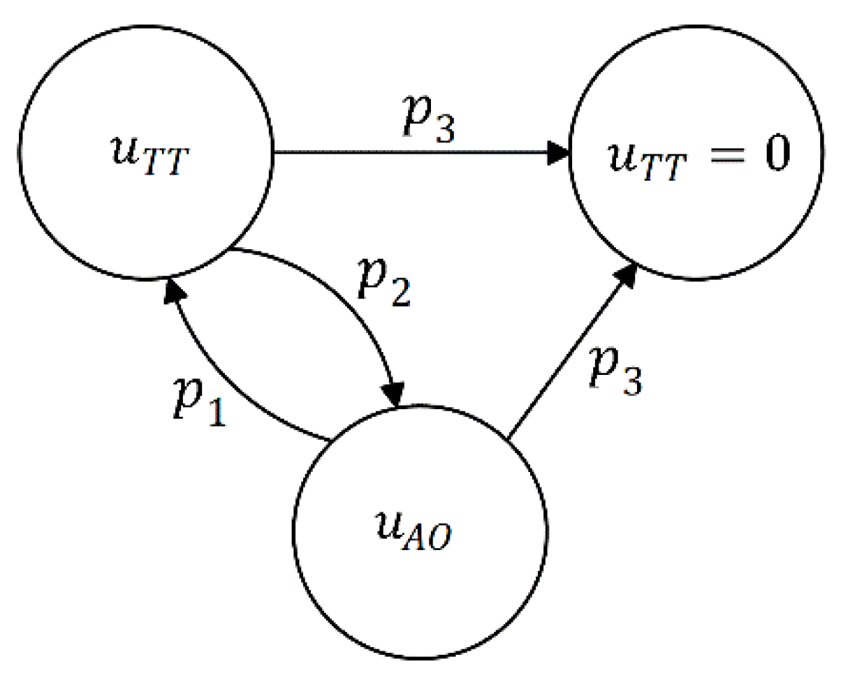
The obstacle avoidance controller is designed to drive the robot to track the desired direction $\beta$, which means that the error $e$ between the desired angle $\beta$ and the current heading orientation $\theta$ converges to zero. The angle $e$ is described as

$$e=\beta -\theta$$

(21)

By differentiating $e$, the error dynamic model can be expressed as

$$\dot{e}=\dot{\beta }-\dot{\theta }=\frac{{\dot{u}}_{y}cos\beta -{\dot{u}}_{x}sin\beta }{\Vert \mathit{u} \Vert }-\omega$$

(22)

A control law for the obstacle avoidance controller is proposed as

$$v=v_r\cos e_3+k_1{e}_1$$

(23)

$$\omega =\frac{{\dot{u}}_{y}cos\beta -{\dot{u}}_{x}sin\beta }{\Vert \mathit{u} \Vert }+k_{2}e$$

(24)

where $k_1$ and $k_2$ are positive control gains.

Notice that the linear velocity of the mobile robot is the same as Equation (2). Combining Equations (14), (18) and (21), the angular velocity of the mobile robot for obstacle avoidance controller can be calculated. Equation (24) can be ultimately converted into a formula without derivative terms, meaning that will not produce possible noise in the obstacle avoidance control.

Substituting Equation (24) into (22), the $\dot{e}$ can be rewritten as

$$\dot{e}=-k_{2}e$$

(25)

Theorem 1.

The error$e$will converge to zero if the control law proposed for obstacle avoidance is chosen as the control inputs of the mobile robot.

Poof of Theorem 1.

Considering a scalar-valued Lyapunov function candidate as

$$V_1=\frac{1}{2}{e}^2$$

(26)

Combining Equation (25), the time derivative of the Lyapunov function candidate $V_1$ can be expressed as

$$\begin{array}{ll}{\dot{V}}_1& =\dot{e}e\\ & =-k_2{e}^2\le 0\end{array}$$

Then, $V_1$ becomes a Lyapunov function, and the controller is asymptotically stable around $e=0$. □

4. Switch Strategy

In this control system, two kinds of dynamics—tracking error dynamics and obstacle avoidance dynamics—are utilized. The previous section has utilized a classic trajectory tracking controller and designed an obstacle avoidance controller. Considering the switch between two controllers, a switch strategy is introduced to combine two controllers.

A transition between two controllers is shown in Figure 3, where $u_{TT}$ and $u_{AO}$ represent the proposed control laws for the trajectory tracking and obstacle avoidance, respectively. The control system of the mobile robot switches different controllers according to the conditions mentioned in the previous section. Considering the practical situation, we define the conditions that represented in the Figure 3 as

$$p_1:\{\begin{array}{c}\Vert {\mathit{u}}_{\mathbf{2}}\Vert >D_{act}\\ {\mathit{u}}_{\mathbf{1}}·{\mathit{u}}_{\mathbf{2}}>0\end{array}$$

where $p_1$ represents the condition that the completion of obstacle avoidance, and it is also used to switch the obstacle avoidance controller to trajectory tracking controller.

$$p_2:\{\begin{array}{l}\Vert {\mathit{u}}_{\mathbf{1}}\Vert <D_{act}\\ p_1 is not satisfied\end{array}$$

where $p_2$ represents the switch condition for control system to activate the obstacle avoidance controller.

$$p_3:\{\begin{array}{c}{v}_r=0\\ {\omega }_r=0\end{array}$$

where $p_3$ represents a condition that the control inputs of the mobile are zero, meaning that the robot will stop moving if the reference velocities of the virtual mobile robot are zero.

The above-mentioned three conditions are used to generate the appropriate control inputs to switch the controllers. At every time epoch, there is only one controller is activated. we can use $q_0$ and $q_1$ to represent the activated state of the trajectory tracking controller and obstacle avoidance controller, respectively. The determination of values of two variables $q_0$ and $q_1$ is the same, which depends on the state of the current controller executed by the control system. As an example, the value of the $q_0$ is 0 or 1, where 1 represents the controller is under activated state, otherwise, the value of $q_0$ is 0.

The control scheme is composed of the two controllers, in order to analysis the stability of this hybrid control system. A total Lyapunov function is defined as

$$V=q_0{V}_0+q_1{V}_1$$

where $V_0$ is the Lyapunov function in [42], and $V_1$ is the Lyapunov function of the obstacle avoidance controller.

The time derivative of the total Lyapunov function is expressed as

$$\dot{V}=q_0{\dot{V}}_0+q_1{\dot{V}}_1$$

(27)

From Equation (27), it can be derived that the derivative of $V$ is ${\dot{V}}_0$ or ${\dot{V}}_1$. Thus, the stability of control system is guaranteed.

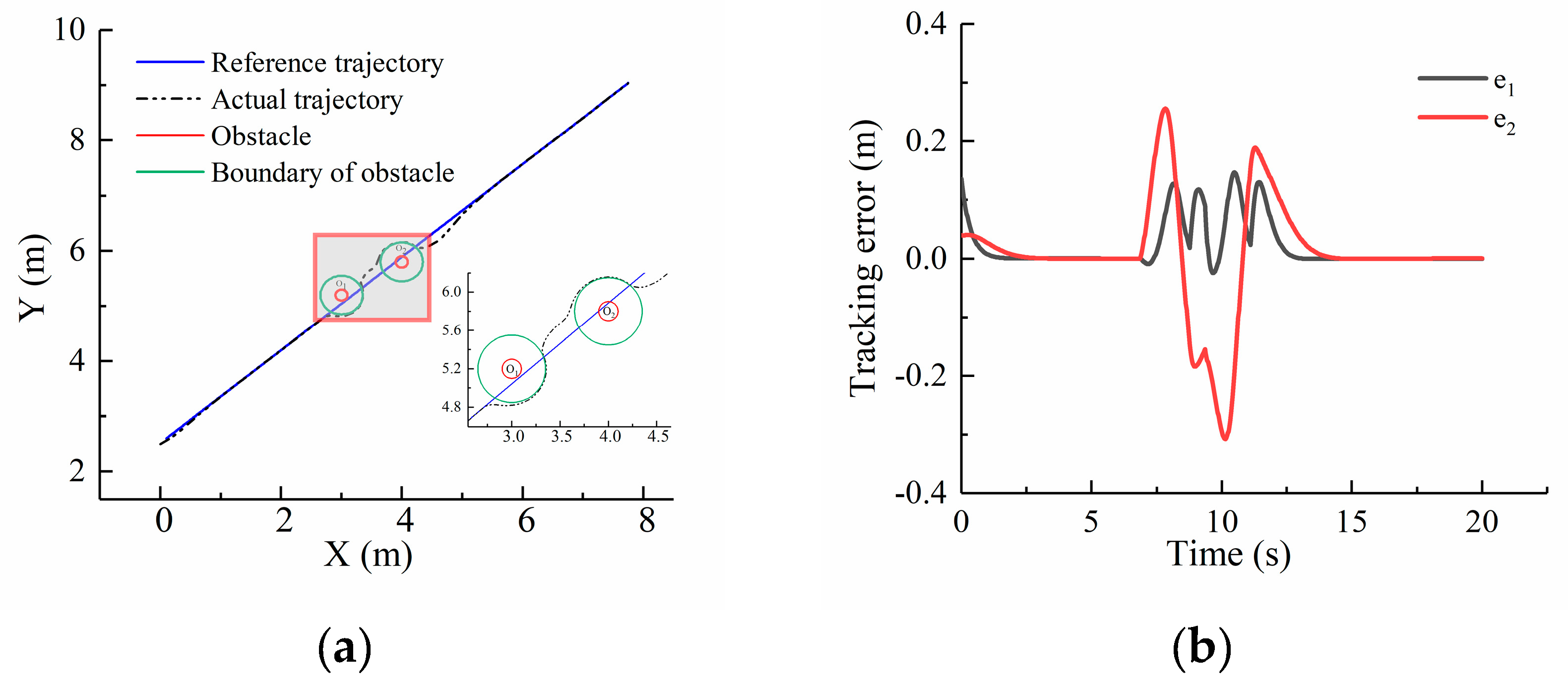
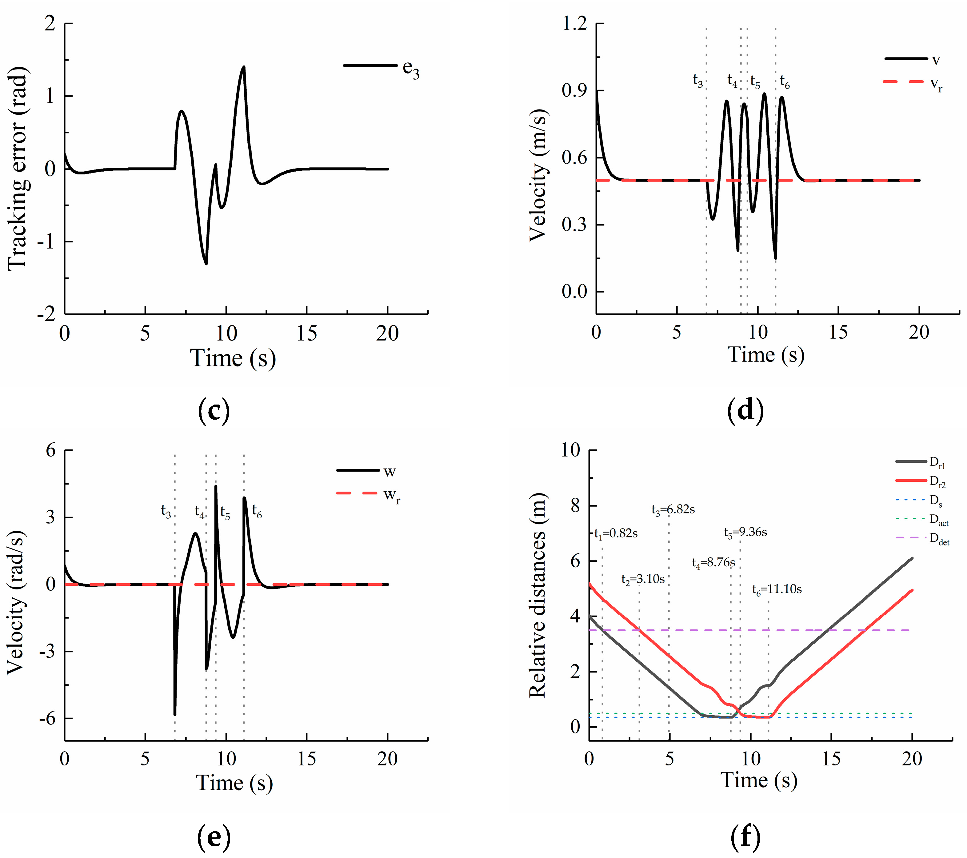
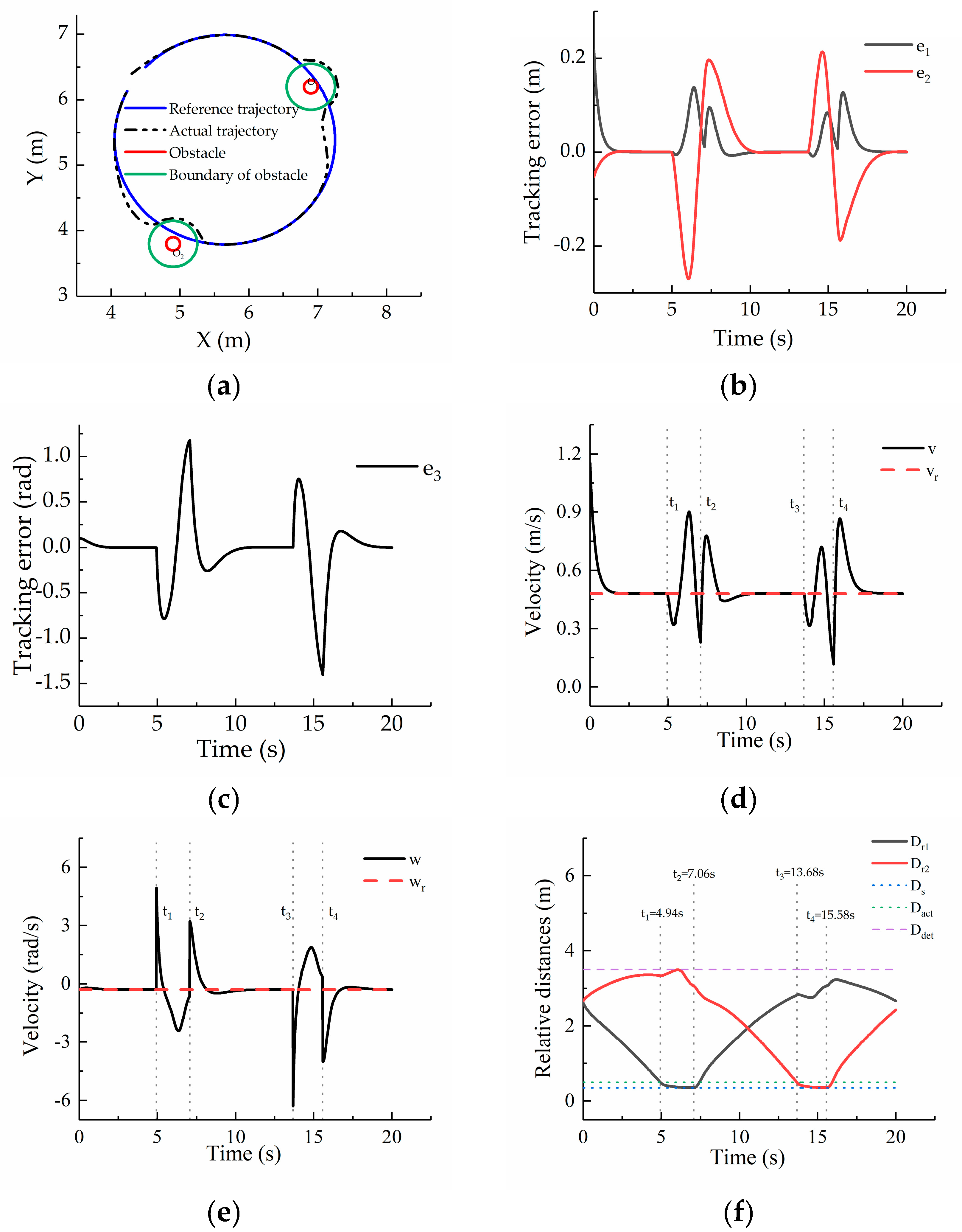
5. Simulation Results and Discussion

Simulations based on the proposed control scheme illustrated in Figure 4 are performed for trajectory tracking in obstacle environments. The simulations are composed of two examples, and two kinds of reference trajectories are utilized. The reference trajectory of the first example is a straight line. The reference trajectory of the second example is circular.

Table 1. Parameters used in two simulations.

Parameter	Description	Value
$R_m$	Radius of the mobile robot	0.2 m
$R_{ob}$	Radius of the obstacle	0.1 m
$D_{det}$	Detected distance of the sensor	3.5 m
$D_{act}$	Distance of activating the obstacle avoidance controller	0.5 m
$D_s$	Safe distance from the obstacle	0.35 m
$k_1,k_2,k_3$	Trajectory tracking control gains	3, 12, 6
$k_1,k_2$	Obstacle avoidance control gains	3, 6

shows the parameters used in two simulations.

The first example is simulated with a straight line. The initial posture of virtual mobile robot is ${\left[\begin{array}{ccc}0.1& 2.6& 0.7\end{array}\right]}^T$, and the reference trajectory is generated by $v_r=0.5\mathrm{m}/\mathrm{s}$ and $w_r=0\mathrm{rad}/\mathrm{s}$. The mobile robot starts to track the virtual mobile robot at the posture ${\left[\begin{array}{ccc}0& 2.5& 0.5\end{array}\right]}^T$. The positions of the obstacles are $O_1\left(3,5.2\right)$ and $O_2\left(4,5.8\right)$, respectively.

Figure 5 shows the simulation results of the first example. At $t_1=0.82 \mathrm{s}$, the mobile robot was tracking trajectory and the obstacle $O_1$ was detected in its working place. The tracking errors $e_1$, $e_2$ and $e_3$ gradually converged to zero, as shown in Figure 5b,c. At $t_2=3.10 \mathrm{s}$, the obstacle $O_2$ was detected. In this case, two obstacles were under the range of the sensors. At $t_3=6.82\mathrm{s}$, the mobile robot moved into the region formed by the $D_{act}$, and the obstacle avoidance controller was activated to drive the robot to its right side to follow the boundary of the obstacle at a constant distance (Figure 5a). The relative distance $D_{r1}$ between the robot and the obstacle $O_1$ kept constant during time period $t_3<t\le t_4$ shown in Figure 5f. At $t_4=8.76 \mathrm{s}$, the reference posture of the virtual mobile robot was outside the region formed by $D_{act}$, and the projection of two vectors ${\mathit{u}}_{\mathbf{1}}$ and ${\mathit{u}}_{\mathbf{2}}$ have same direction in x-axis. Obstacle avoidance can be considered as being completed, and the controller was switched from the obstacle avoidance controller to the trajectory tracking controller. The mobile robot gone on tracking the reference trajectory. After this moment, the relative distance $D_{r2}$ between the mobile robot and the obstacle $O_2$ gradually decreased. At $t_5=9.36\mathrm{s}$, $D_{r2}\le D_s$, the trajectory tracking controller was stopped and the obstacle avoidance controller was activated. As shown in Figure 5a,f, the robot moved towards its left side to follow the boundary of the obstacle and kept a constant distance $D_s$ to the obstacle $O_2$ during time period $t_5<t\le t_6$. At $t_6=11.10\mathrm{s}$, the condition of completion of obstacle avoidance was satisfied, the trajectory tracking controller was performed, the relative distance $D_{r2}$ gradually increased, and the tracking errors gradually decreased to zero (Figure 5b,c), which meant that the robot had escaped the obstacle and started the tracking. During the whole moving process, the relative distances $D_{r1}$ and $D_{r2}$ always satisfied the conditions $D_{r1}\ge D_s$ and $D_{r2}\ge D_s$. Therefore, there is no collision occurred between the robot and the obstacles. The control inputs of the mobile robot in whole simulation are shown in Figure 5d,e.

To further validate the effectiveness of the proposed control strategy, the second example is performed with a circular trajectory. The initial posture of the reference trajectory is ${\left[\begin{array}{ccc}4.5& 6.5& 0.8\end{array}\right]}^T$, and the reference trajectory is generated by $v_r=0.48\mathrm{m}/\mathrm{s}$ and $w_r=-0.3\mathrm{rad}/\mathrm{s}$. The initial posture of the mobile robot is ${\left[\begin{array}{ccc}4.3& 6.4& 0.7\end{array}\right]}^T$. The positions of the obstacles are $O_1\left(6.9,6.2\right)$ and $O_2\left(4.9,3.8\right)$, respectively.

Figure 6 shows the results of the second example. Before $t_1=4.94 \mathrm{s}$, the mobile tracked the desired trajectory and detected the obstacles $O_{1 }$ and $O_2$. At $t_1=4.94\mathrm{s}$, the relative distance $D_{r1}$ between the robot and the obstacle $O_1$ satisfied the condition $D_{r1}\le D_{act}$. The control system activated the obstacle avoidance controller to drive the robot to its left side to follow the boundary of the obstacle $O_1$, and the mobile robot kept a constant distance $D_s$ to the obstacle $O_1$ before the completion of obstacle avoidance (Figure 6a,f). After $t_2=7.06\mathrm{s}$, the controller executed by the control system was switched to the trajectory tracking controller. As shown in Figure 6b,c, the tracking errors gradually converged to zero during $t_2<t\le t_3$. At $t_3=13.68 \mathrm{s}$, the obstacle avoidance controller was activated. The mobile robot moved towards its right side to follow the boundary of the obstacle $O_2$ during $t_3<t\le t_4$. At $t_4=15.58 \mathrm{s}$, the obstacle avoidance with the obstacle $O_2$ was completed, and the trajectory tracking controller was activated to track the reference trajectory. As shown in Figure 6f, the relative distances between the robot and two obstacles represented by $D_{r1}$ and $D_{r2}$ always satisfied the conditions $D_{r1}\ge D_s$ and $D_{r2}\ge D_s$. This shows that no collision occurred in unknown obstacle environments. The control inputs of the mobile robot are given in Figure 6d,e, and tracking errors are shown in Figure 6b,c.

From the results of two simulation scenarios, it can be concluded that the mobile robot can track the trajectory before encountering obstacles in the environment. Once an obstacle is detected by the sensors attached to the mobile robot, the safe boundary and risk area of an obstacle are generated by the obstacle avoidance controller. When the robot moves into the region form by an activated distance, the obstacle avoidance controller is activated to determine the fastest obstacle avoidance direction to follow the obstacle boundary at a constant safe distance, and then after the completion of the obstacle avoidance, a transition between trajectory tracking and obstacle avoidance is triggered. The mobile robot goes on to track, and the tracking errors gradually decrease to zero. This combination of two controllers can well address the problem of trajectory tracking in obstacle environments. Therefore, the proposed scheme can be applied to the mobile robot to track the trajectory while considering obstacles.

6. Conclusions

In this paper, a control scheme consisting of the trajectory tracking and obstacle avoidance controllers is proposed to address the trajectory tracking problem in unknown obstacle environments. The trajectory tracking controller is employed to track pre-planned trajectory based on its tracking error dynamics. To deal with the problem of the possible obstacles in the environment, a blending vector is introduced to control the mobile robot toward the fastest obstacle avoidance direction to follow the boundary of an obstacle at a constant distance to escape the obstacle. Finally, two controllers combined by a switch strategy are switched to calculate the control inputs to track the trajectory or avoid the obstacle.

The results obtained from simulations indicate that the proposed control scheme can effectively ensure the safe movement of the mobile robot. In brief, the proposed control scheme provides a new simple method with application values for solving the tracking problem in unknown obstacle environments. However, this article does not consider dynamic obstacles and external disturbances existing in the environment. For future work, we will focus on the extension of the proposed control scheme to dynamical environments filled with disturbances.

References

1. Zhao, J.C.; Gao, J.Y.; Zhao, F.Z.; Liu, Y. A Search-and-Rescue Robot System for Remotely Sensing the Underground Coal Mine Environment. Sensors 2017, 17, 2426. [Google Scholar] [CrossRef] [Green Version]
2. Kowalczyk, W. Formation Control and Distributed Goal Assignment for Multi-Agent Non-Holonomic Systems. Appl. Sci. 2019, 9, 23. [Google Scholar] [CrossRef] [Green Version]
3. Consolini, L.; Morbidi, F.; Prattichizzo, D.; Tosques, M. Leader-follower formation control of nonholonomic mobile robots with input constraints. Automatica 2008, 44, 1343–1349. [Google Scholar] [CrossRef]
4. Galasso, F.; Rizzini, D.L.; Oleari, F.; Caselli, S. Efficient calibration of four wheel industrial AGVs. Robot. Comput. Integr. Manuf. 2019, 57, 116–128. [Google Scholar] [CrossRef]
5. Villagra, J.; Herrero-Perez, D. A Comparison of Control Techniques for Robust Docking Maneuvers of an AGV. IEEE Trans. Control Syst. Technol. 2012, 20, 1116–1123. [Google Scholar] [CrossRef]
6. Bhat, S.; Meenakshi, M. Military Robot Path Control Using RF Communication. Proc. First Int. Conf. Intell. Comput. Commun. 2017, 458, 697–704. [Google Scholar] [CrossRef]
7. Adamczyk, M.; Bulandra, K.; Moczulski, W. Autonomous mobile robotic system for supporting counterterrorist and surveillance operations. In Counterterrorism, Crime Fighting, Forensics, and Surveillance Technologies; Bouma, H., CarlysleDavies, F., Stokes, R.J., Yitzhaky, Y., Eds.; Spie-Int Soc Optical Engineering: Bellingham, WA, USA, 2017; Volume 10441. [Google Scholar]
8. Ali, M.A.H.; Mailah, M. Path Planning and Control of Mobile Robot in Road Environments Using Sensor Fusion and Active Force Control. IEEE Trans. Veh. Technol. 2019, 68, 2176–2195. [Google Scholar] [CrossRef]
9. Rostami, S.M.H.; Sangaiah, A.K.; Wang, J.; Liu, X.Z. Obstacle avoidance of mobile robots using modified artificial potential field algorithm. Eurasip J. Wirel. Commun. Netw. 2019, 19. [Google Scholar] [CrossRef] [Green Version]
10. Orozco-Rosas, U.; Montiel, O.; Sepulveda, R. Mobile robot path planning using membrane evolutionary artificial potential field. Appl. Soft Comput. 2019, 77, 236–251. [Google Scholar] [CrossRef]
11. Xue, Y. Mobile Robot Path Planning with a Non-Dominated Sorting Genetic Algorithm. Appl. Sci. 2018, 8, 27. [Google Scholar] [CrossRef] [Green Version]
12. Elhoseny, M.; Tharwat, A.; Hassanien, A.E. Bezier Curve Based Path Planning in a Dynamic Field using Modified Genetic Algorithm. J. Comput. Sci. 2018, 25, 339–350. [Google Scholar] [CrossRef]
13. Nazarahari, M.; Khanmirza, E.; Doostie, S. Multi-objective multi-robot path planning in continuous environment using an enhanced genetic algorithm. Expert Syst. Appl. 2019, 115, 106–120. [Google Scholar] [CrossRef]
14. Antonakis, A.; Nikolaidis, T.; Pilidis, P. Multi-Objective Climb Path Optimization for Aircraft/Engine Integration Using Particle Swarm Optimization. Appl. Sci. 2017, 7, 22. [Google Scholar] [CrossRef] [Green Version]
15. Yang, H.; Qi, J.; Miao, Y.C.; Sun, H.X.; Li, J.H. A New Robot Navigation Algorithm Based on a Double-Layer Ant Algorithm and Trajectory Optimization. IEEE Trans. Ind. Electron. 2019, 66, 8557–8566. [Google Scholar] [CrossRef] [Green Version]
16. Lin, T.C.; Chen, C.C.; Lin, C.J. Wall-following and Navigation Control of Mobile Robot Using Reinforcement Learning Based on Dynamic Group Artificial Bee Colony. J. Intell. Robot. Syst. 2018, 92, 343–357. [Google Scholar] [CrossRef]
17. Matveev, A.S.; Wang, C.; Saykin, A.V. Real-time navigation of mobile robots in problems of border patrolling and avoiding collisions with moving and deforming obstacles. Robot. Auton. Syst. 2012, 60, 769–788. [Google Scholar] [CrossRef]
18. Wang, C.; Savkin, A.V.; Garratt, M. A strategy for safe 3D navigation of non-holonomic robots among moving obstacles. Robotica 2018, 36, 275–297. [Google Scholar] [CrossRef]
19. Thanh, H.; Phi, N.N.; Hong, S.K. Simple nonlinear control of quadcopter for collision avoidance based on geometric approach in static environment. Int. J. Adv. Robot. Syst. 2018, 15, 17. [Google Scholar] [CrossRef] [Green Version]
20. Maurovic, I.; Baotic, M.; Petrovic, I. Explicit Model Predictive Control for Trajectory Tracking with Mobile Robots. In Proceedings of the 2011 IEEE/ASME International Conference on Advanced Intelligent Mechatronics, Budapest, Hungary, 3–7 July 2011; IEEE: New York, NY, USA, 2011; pp. 712–717. [Google Scholar]
21. Klancar, G.; Krjanc, I. Tracking-error model-based predictive control for mobile robots in real time. Robot. Auton. Syst. 2007, 55, 460–469. [Google Scholar] [CrossRef]
22. Kumar, P.; Anoohya, B.B.; Padhi, R. Model Predictive Static Programming for Optimal Command Tracking: A Fast Model Predictive Control Paradigm. J. Dyn. Syst. Meas. Control. Trans. ASME 2019, 141, 12. [Google Scholar] [CrossRef]
23. Woo, C.; Lee, M.; Yoon, T. Robust Trajectory Tracking Control of a Mecanum Wheeled Mobile Robot Using Impedance Control and Integral Sliding Mode Control. J. Korea Robot. Soc. 2018, 13, 256–264. [Google Scholar] [CrossRef]
24. Sahloul, S.; Benhalima, D.; Rekik, C. Tracking trajectory of a mobile robot using sliding mode control. In Proceedings of the 2018 15th International Multi-Conference on Systems, Signals And Devices, Hammamet, Tunisia, 19–22 March 2018; IEEE: Piscataway, NJ, USA, 2018; pp. 1386–1390. [Google Scholar]
25. Goswami, N.K.; Padhy, P.K. Sliding mode controller design for trajectory tracking of a non-holonomic mobile robot with disturbance. Comput. Electr. Eng. 2018, 72, 307–323. [Google Scholar] [CrossRef]
26. Mu, J.Q.; Yan, X.G.; Spurgeon, S.K.; Mao, Z.H. Generalized Regular Form Based SMC for Nonlinear Systems With Application to a WMR. IEEE Trans. Ind. Electron. 2017, 64, 6714–6723. [Google Scholar] [CrossRef] [Green Version]
27. Falsafi, M.H.; Alipour, K.; Tarvirdizadeh, B. Tracking-Error Fuzzy-Based Control for Nonholonomic Wheeled Robots. Arab. J. Sci. Eng. 2019, 44, 881–892. [Google Scholar] [CrossRef]
28. Abbas, M.A.; Milman, R.; Eklund, J.M. Obstacle Avoidance in Real Time With Nonlinear Model Predictive Control of Autonomous Vehicles. Can. J. Electr. Comput. Eng. Rev. Can. Genie Electr. Inform. 2017, 40, 12–22. [Google Scholar] [CrossRef]
29. Castillo, O.; Martinez-Marroquin, R.; Melin, P.; Valdez, F.; Soria, J. Comparative study of bio-inspired algorithms applied to the optimization of type-1 and type-2 fuzzy controllers for an autonomous mobile robot. Inf. Sci. 2012, 192, 19–38. [Google Scholar] [CrossRef]
30. Shu, P.F.; Oya, M.; Zhao, J.J. A new adaptive tracking control scheme of wheeled mobile robot without longitudinal velocity measurement. Int. J. Robust Nonlinear Control 2018, 28, 1789–1807. [Google Scholar] [CrossRef]
31. Cui, M.Y.; Liu, H.Z.; Liu, W.; Qin, Y. An Adaptive Unscented Kalman Filter-based Controller for Simultaneous Obstacle Avoidance and Tracking of Wheeled Mobile Robots with Unknown Slipping Parameters. J. Intell. Robot. Syst. 2018, 92, 489–504. [Google Scholar] [CrossRef]
32. Wang, Y.; Shuoyu, W.; Tan, R.; Jiang, Y. Adaptive control method for path tracking of wheeled mobile robot considering parameter changes. Int. J. Adv. Mechatron. Syst. 2012, 4, 41–49. [Google Scholar] [CrossRef]
33. Rahmani, B.; Belkheiri, M. Adaptive neural network output feedback control for flexible multi-link robotic manipulators. Int. J. Control 2019, 92, 2324–2338. [Google Scholar] [CrossRef]
34. Abdelhakim, G.; Abdelouahab, H. A New Approach for Controlling a Trajectory Tracking Using Intelligent Methods. J. Electr. Eng. Technol. 2019, 14, 1347–1356. [Google Scholar] [CrossRef]
35. Yoo, S.J. Adaptive tracking and obstacle avoidance for a class of mobile robots in the presence of unknown skidding and slipping. IET Control Theory Appl. 2011, 5, 1597–1608. [Google Scholar] [CrossRef]
36. Yang, H.J.; Fan, X.Z.; Shi, P.; Hua, C.C. Nonlinear Control for Tracking and Obstacle Avoidance of a Wheeled Mobile Robot With Nonholonomic Constraint. IEEE Trans. Control Syst. Technol. 2016, 24, 741–746. [Google Scholar] [CrossRef] [Green Version]
37. Kowalczyk, W.; Michalek, M.; Kozlowski, K. Trajectory tracking control with obstacle avoidance capability for unicycle-like mobile robot. Bull. Pol. Acad. Sci. Tech. Sci. 2012, 60, 537–546. [Google Scholar] [CrossRef] [Green Version]
38. Ji, J.; Khajepour, A.; Melek, W.W.; Huang, Y. Path planning and tracking for vehicle collision avoidance based on model predictive control with multiconstraints. IEEE Trans. Veh. Technol. 2017, 66, 952–964. [Google Scholar] [CrossRef]
39. Ha, L.N.N.T.; Bui, D.H.P.; Hong, S.K. Nonlinear Control for Autonomous Trajectory Tracking while Considering Collision Avoidance of UAVs Based on Geometric Relations. Energies 2019, 12, 1551. [Google Scholar] [CrossRef] [Green Version]
40. Tzafestas, S.G. Mobile Robot Control and Navigation: A Global Overview. J. Intell. Robot. Syst. 2018, 91, 35–58. [Google Scholar] [CrossRef]
41. Thanh, H.L.N.N.; Hong, S.K. Completion of Collision Avoidance Control Algorithm for Multicopters Based on Geometrical Constraints. IEEE Access 2018, 6, 27111–27126. [Google Scholar] [CrossRef]
42. Kanayama, Y.; Kimura, Y.; Miyazaki, F.; Noguchi, T. A stable tracking control method for an autonomous mobile robot. In Proceedings of the IEEE International Conference on Robotics and Automation, Cincinnati, OH, USA, 13–18 May 1990; Volume 381, pp. 384–389. [Google Scholar]
Figure 1. Diagram of trajectory tracking.
Electronics 09 00042 g001
Figure 2. Geometrical relations between the robot and the obstacle: (a) The detection of an obstacle; (b) The completion of obstacle avoidance.
Electronics 09 00042 g002
Figure 3. Switch strategy of the proposed control system.
Electronics 09 00042 g003
Figure 4. Structure of the proposed control scheme for the mobile robot.
Electronics 09 00042 g004
Figure 5. Simulation results of the first example: (a) Trajectory tracking and obstacle avoidance results; (b) position tracking error; (c) angular tracking error; (d) control input v and reference velocity v r ; (e) control input ω and reference velocity ω r ; (f) relative distances between the robot and obstacles.
Electronics 09 00042 g005aElectronics 09 00042 g005b
Figure 6. Simulation results of the second example: (a) trajectory tracking and obstacle avoidance results; (b) position tracking error; (c) angular tracking error; (d) control input v and reference velocity v r ; (e) control input ω and reference velocity ω r ; (f) relative distances between the robot and obstacles.
Electronics 09 00042 g006