Vehicular Navigation Based on the Fusion of 3D-RISS and Machine Learning Enhanced Visual Data in Challenging Environments


Abstract
1. Introduction
2. Formulation
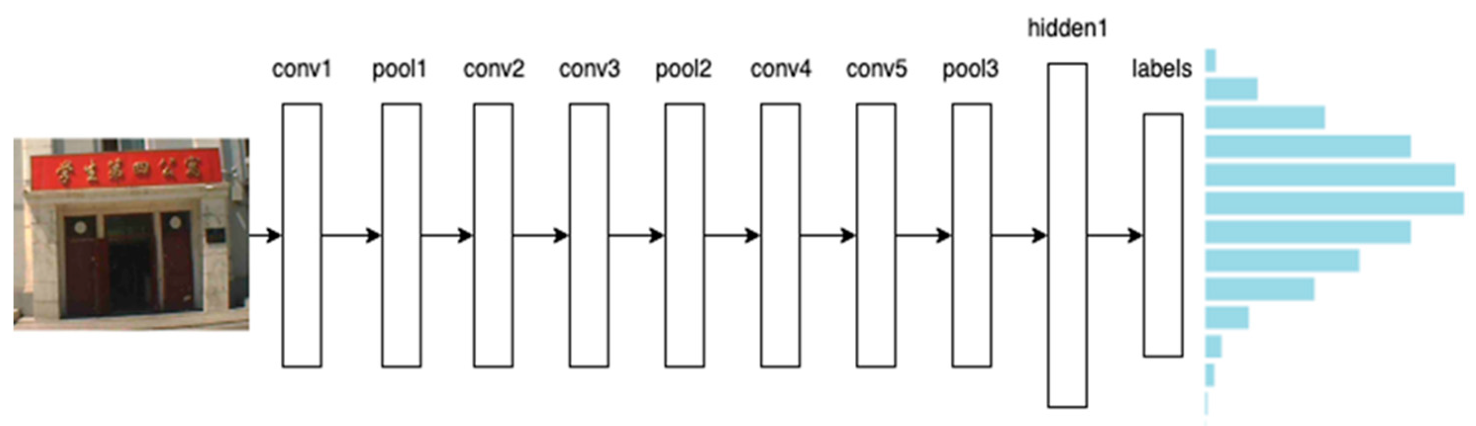
2.1. Convolution Neural Network
2.2. Visual System
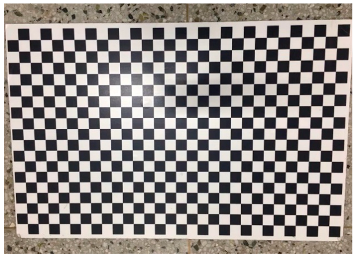
2.2.1. Camera Calibration and Correction of Distorted Image
2.2.2. Template Matching
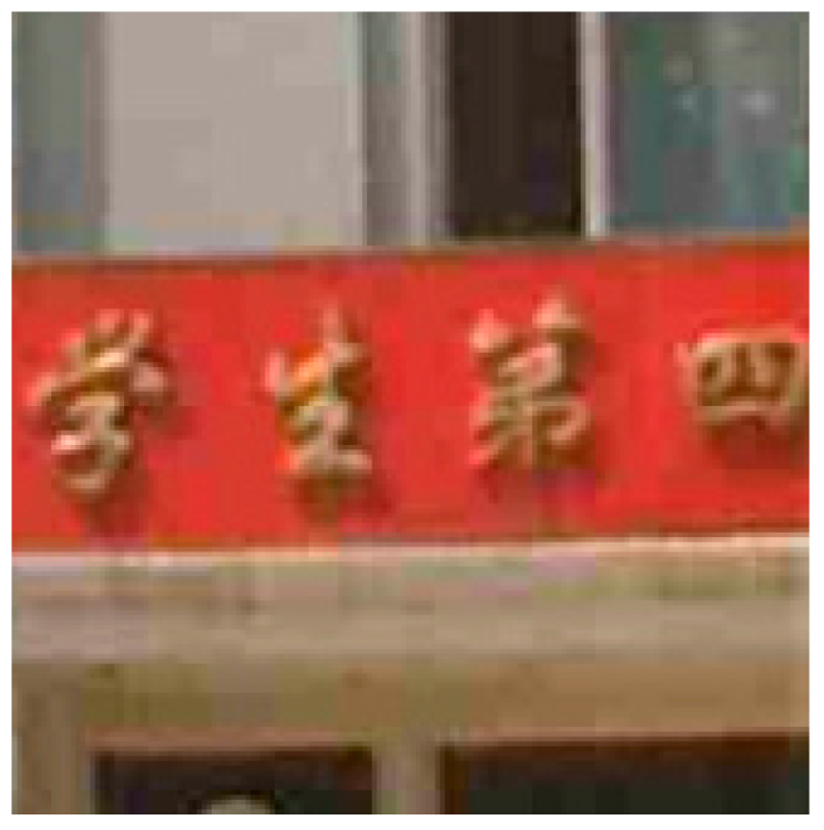
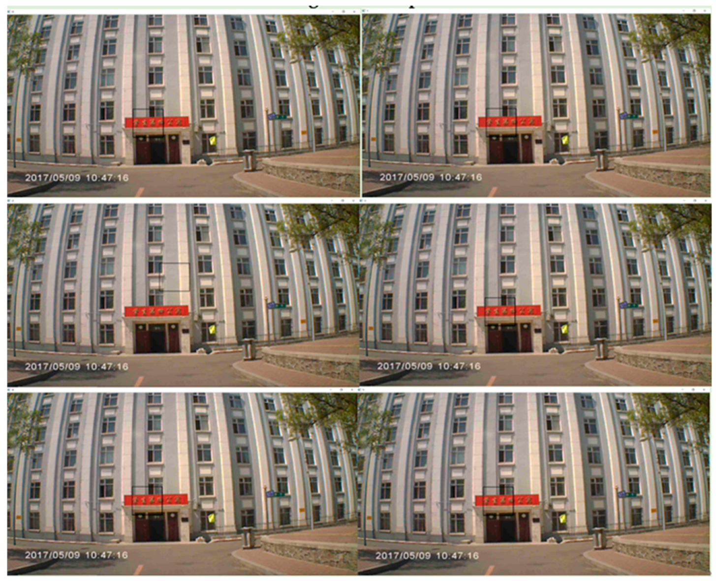
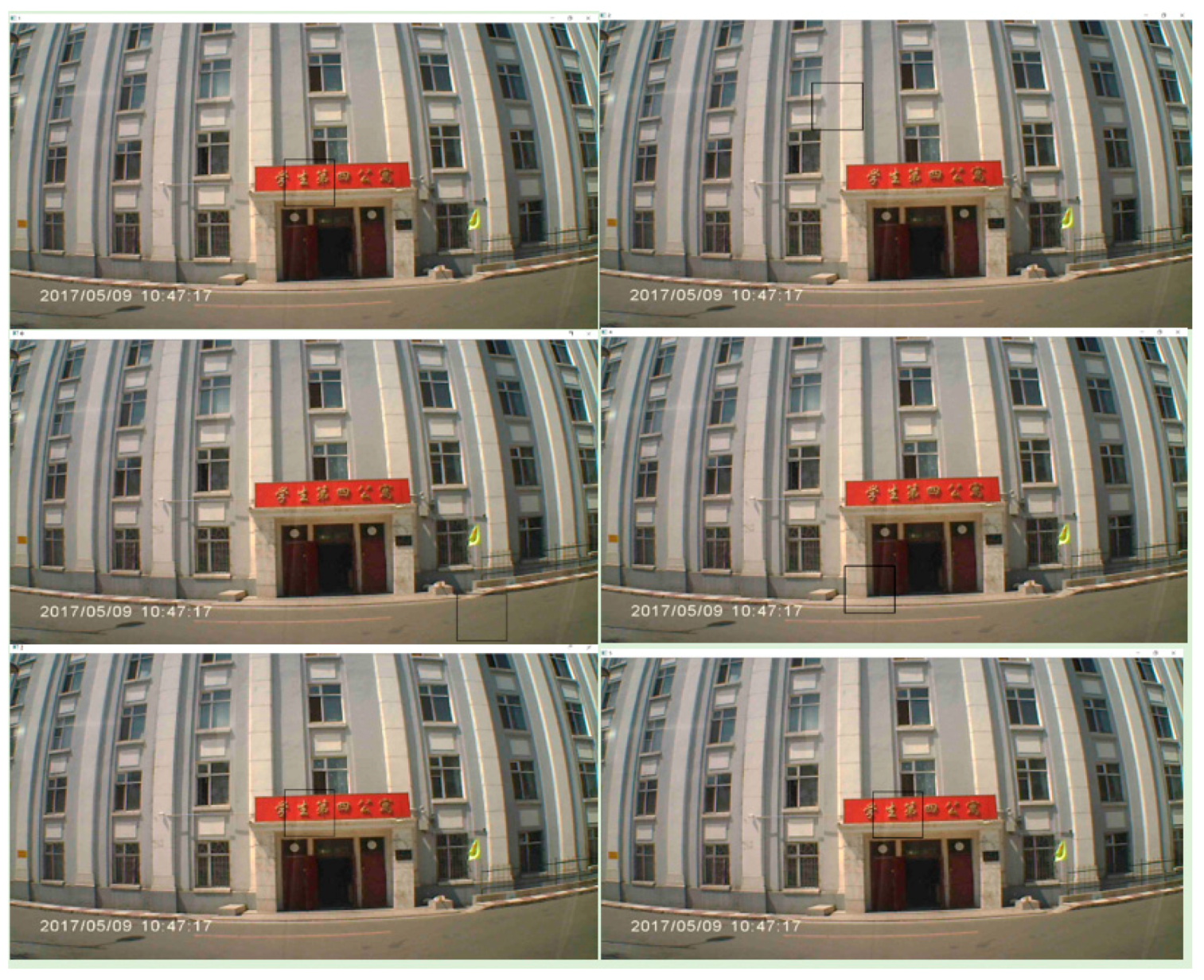
2.2.3. Landmark Chosen
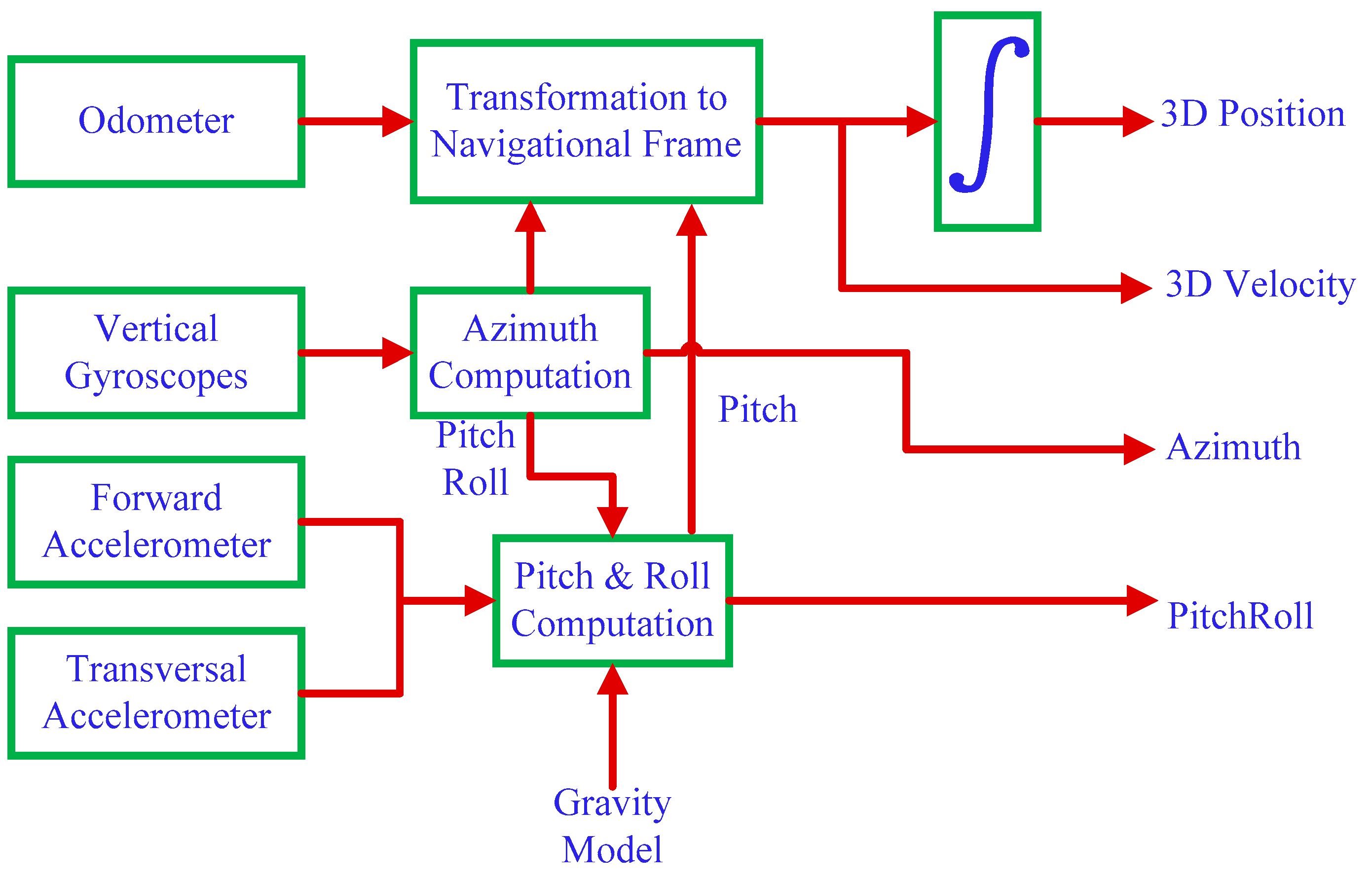
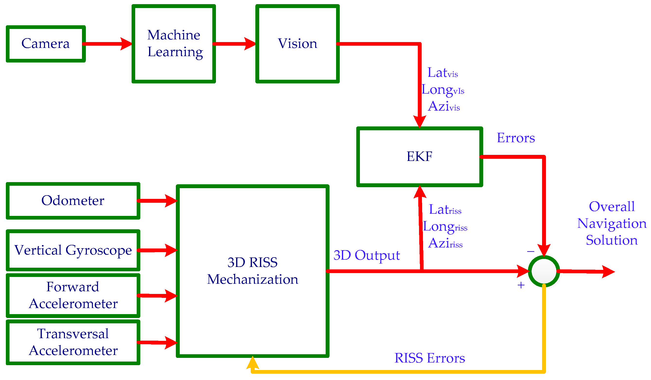
2.3. 3D-RISS Mechanization
2.4. Kalman Filter Design of 3D-RISS/MLEVD Integration
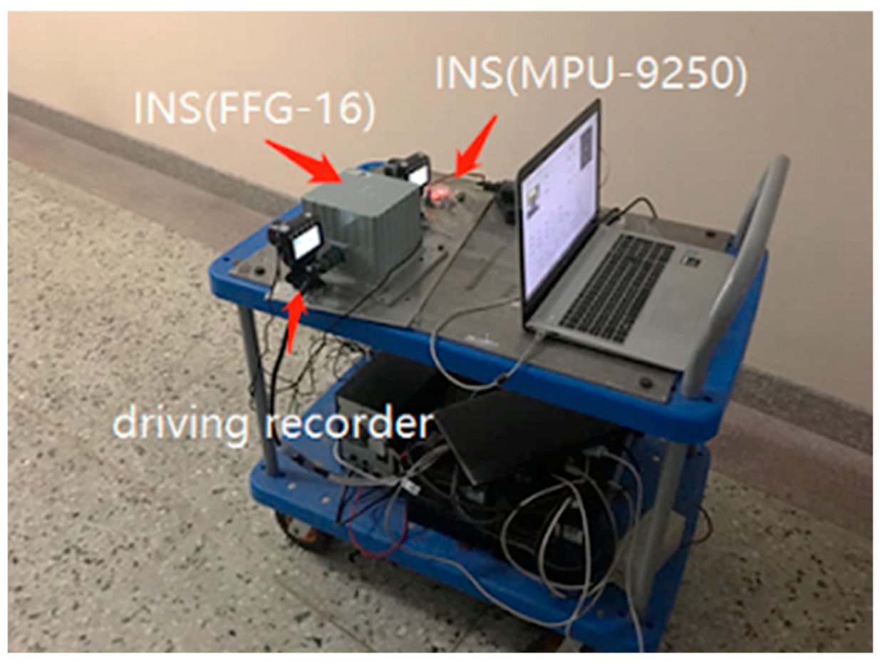
3. Verification Experiments and Results Analysis
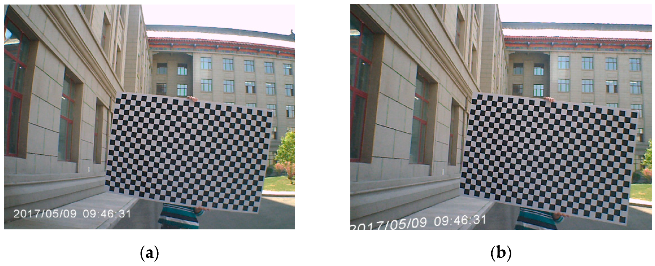
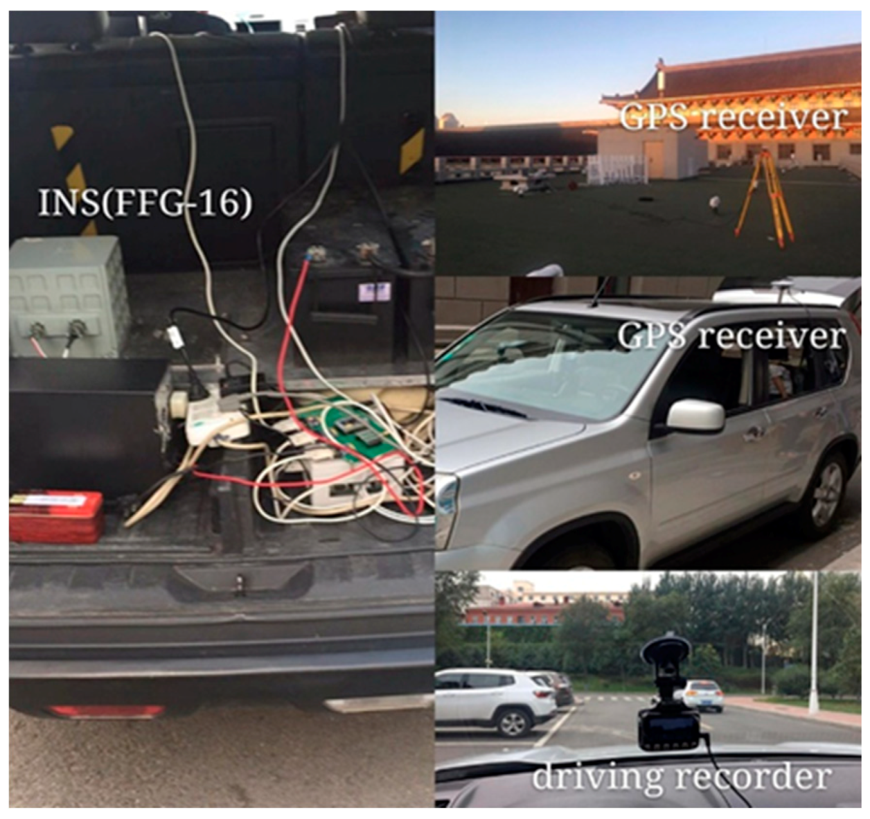
3.1. Outdoor Experiment
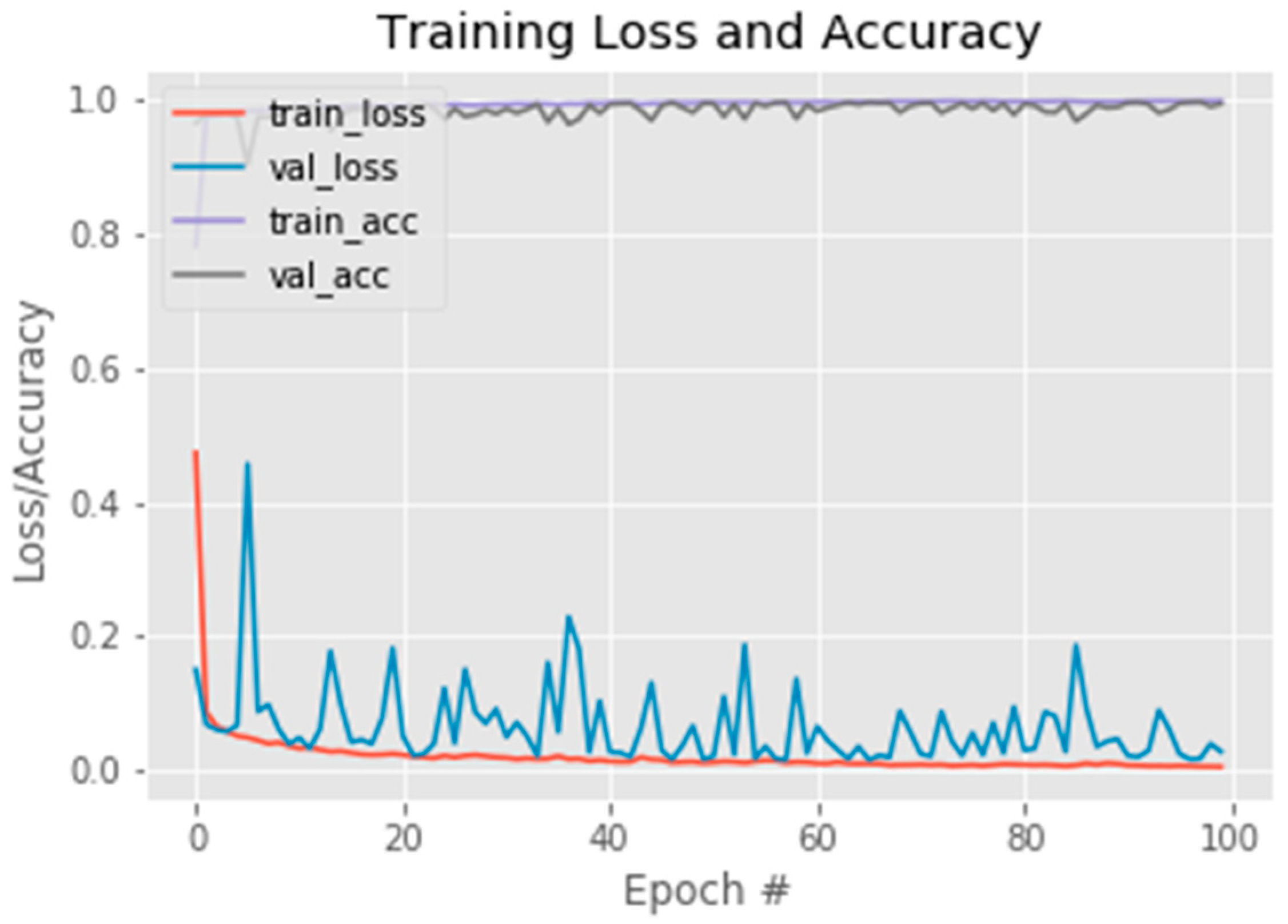
3.1.1. Selecting Pictures by Machine Learning
3.1.2. Template Matching
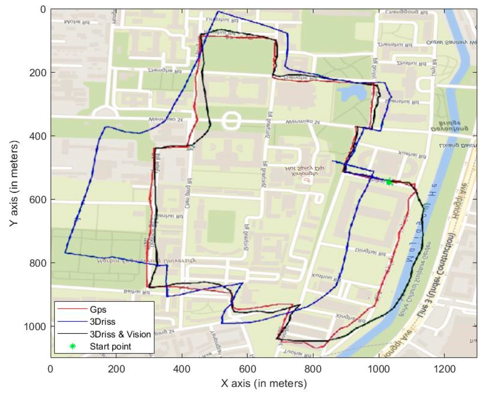
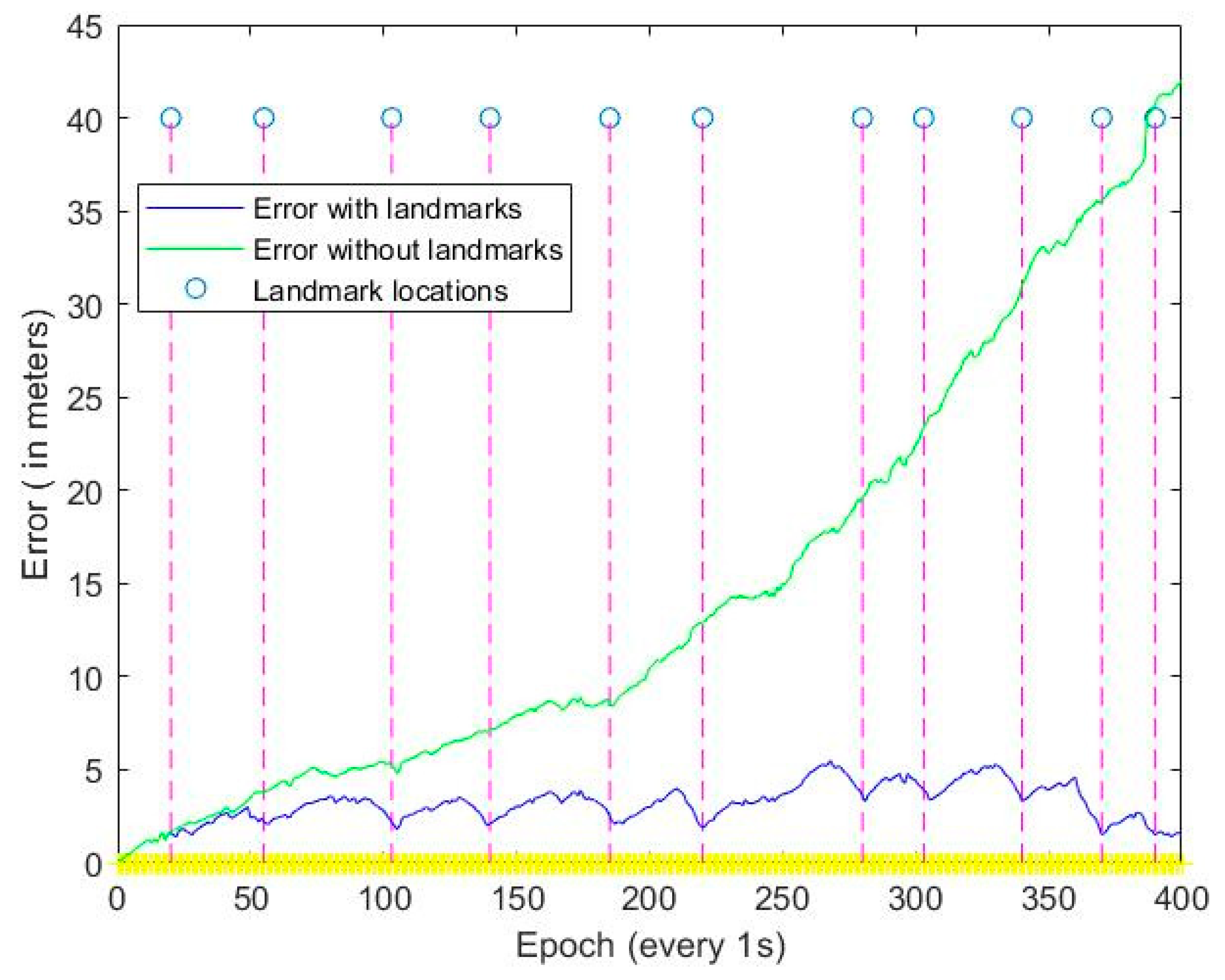
3.1.3. 3D-RISS and Vision Integration
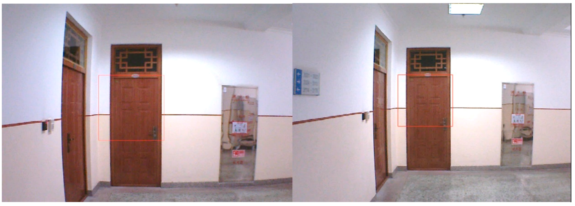
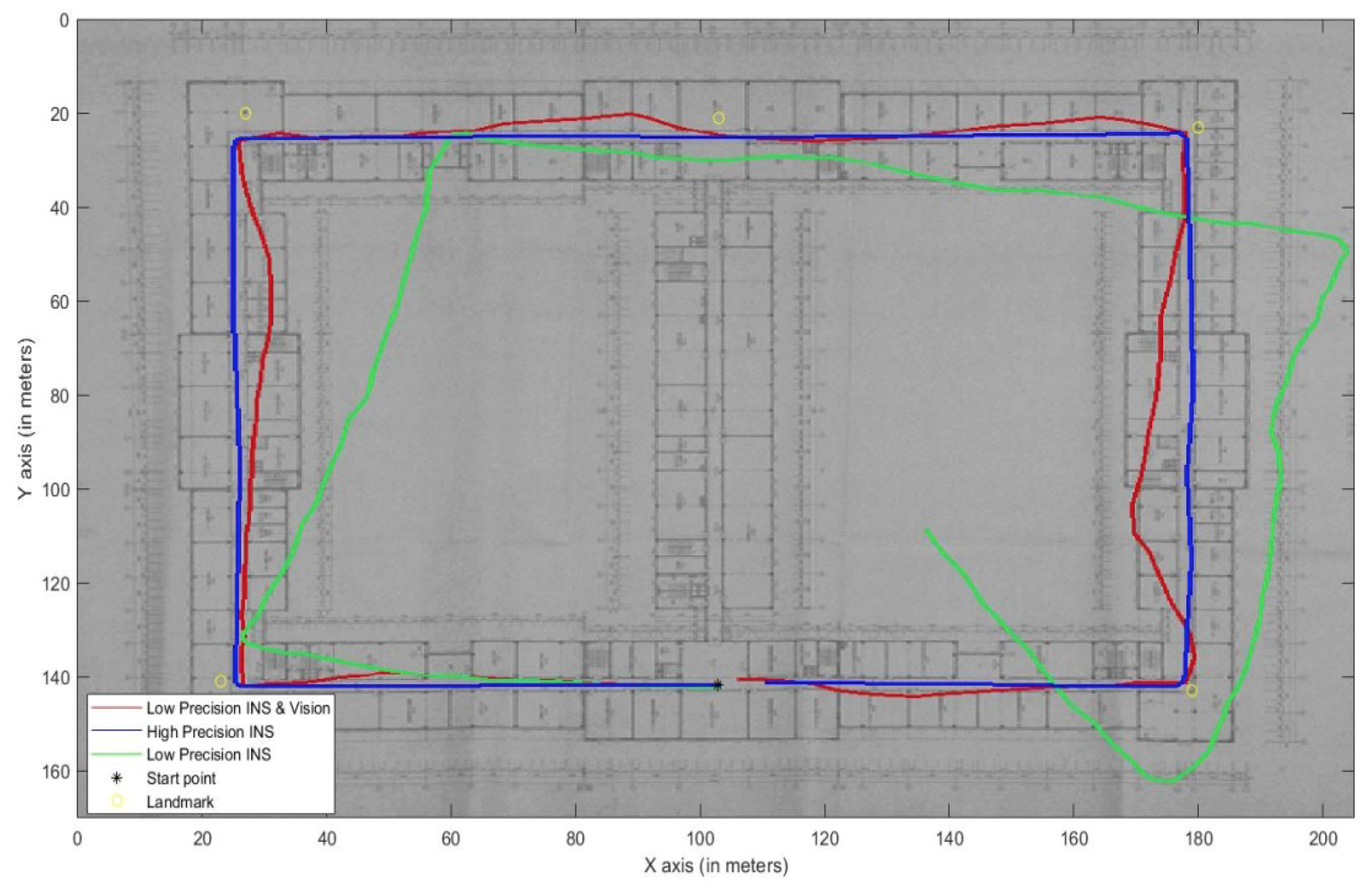
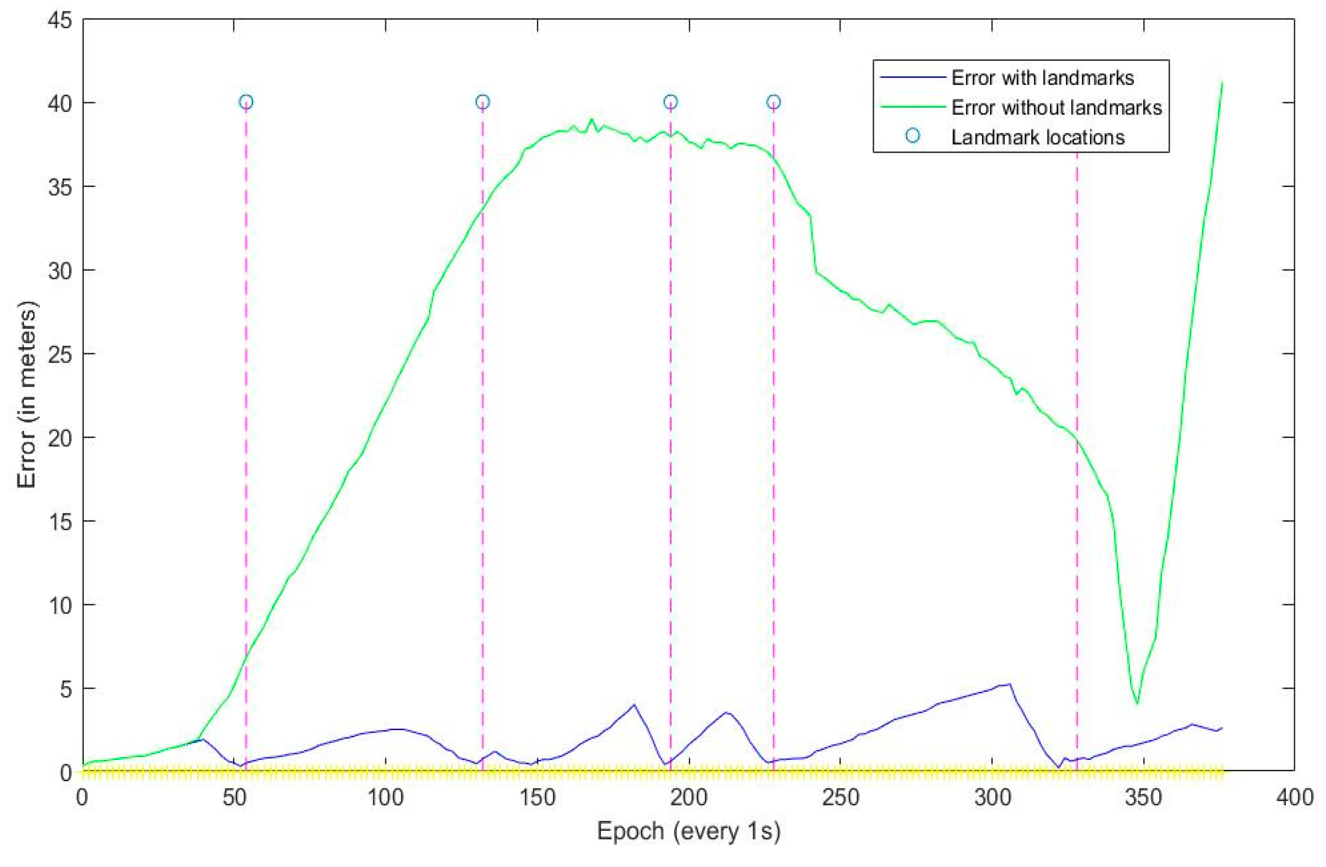
3.2. Indoor Experiment
4. Conclusions
Author Contributions
Funding
Acknowledgments
Conflicts of Interest
References
- Misra, P.; Enge, P. Global Positioning System: Signals, Measurements, and Performance; Ganga-Jamuna Press: Lincoln, MA, USA, 2011. [Google Scholar]
- Nerem, R.S.; Larson, K.M. Global Positioning System, Theory and Practice. Eos Trans. Am. Geophys. Union 2001, 82, 365. [Google Scholar] [CrossRef]
- Titterton, D.; Weston, J. Strapdown Inertial Navigation Technology; The Institution of Electrical Engineers: London, UK, 2004. [Google Scholar]
- Mainone, M.; Cheng, Y.; Matthies, L. Two years of visual odometer on the mars exploration rovers. J. Field Robot. Spec. Issue Space Robot. 2007, 24, 169–186. [Google Scholar] [CrossRef]
- Zhong, Z.; Yi, J.; Zhao, D. Novel approach for mobile robot localization using monocular vision. Proc. SPIE 2003, 5286, 159–162. [Google Scholar]
- Sun, Y.; Rahman, M. Integrating Vision Based Navigation with INS and GPS for Land Vehicle Navigation in Challenging GNSS Environments. In Proceedings of the 29th International Technical Meeting of the Satellite Division of The Institute of Navigation, Portland, OR, USA, 12–16 September 2016. [Google Scholar]
- Martinelli, A.; Siegwart, R. Vision and IMU Data Fusion: Closed-Form Determination of the Absolute Scale, Speed, and Attitude. In Handbook of Intelligent Vehicles; Springer: London, UK, 2012; pp. 1335–1354. [Google Scholar]
- Wang, W. Research of Ego-Positioning for Micro Air Vehicles Based on Monocular Vision and Inertial Measurement. J. Jilin Univ. 2016, 34, 774–780. [Google Scholar]
- Zhao, S.; Lin, F.; Peng, K. Vision-aided Estimation of Attitude, Velocity, and Inertial Measurement Bias for UAV Stabilization. J. Intell. Robot. Syst. 2016, 81, 531–549. [Google Scholar] [CrossRef]
- Schmidhuber, J. Deep Learning in Neural Networks: An Overview. Neural Netw. 2015, 61, 85–117. [Google Scholar] [CrossRef]
- Mnih, V.; Heess, N.; Graves, A. Recurrent Models of Visual Attention. In Proceedings of the NIPS’14: 27th International Conference on Neural Information Processing Systems, Montreal, QC, Canada, 8–13 December 2014. [Google Scholar]
- Karpathy, A.; Joulin, A.; Li, F. Deep Fragment Embeddings for Bidirectional Image Sentence Mapping. In Proceedings of the International Conference on Neural Information Processing Systems, Montreal, QC, Canada, 8–13 December 2014; MIT Press: Cambridge, MA, USA, 2014. [Google Scholar]
- Goodfellow, I.J.; Bulatov, Y.; Ibarz, J. Multi-digit Number Recognition from Street View Imagery using Deep Convolutional Neural Networks. arXiv 2013, arXiv:1312.6082. [Google Scholar]
- Vinyals, O.; Toshev, A.; Bengio, S. Show and Tell: A Neural Image Caption Generator. In Proceedings of the IEEE Conference on Computer Vision and Pattern Recognition, San Juan, PR, USA, 17–19 June 1997. [Google Scholar]
- Krizhevsky, A.; Sutskever, I.; Hinton, G. ImageNet Classification with Deep Convolutional Neural Networks, NIPS; Curran Associates Inc.: Red Hook, NY, USA, 2012. [Google Scholar]
- Lecun, Y.; Bengio, Y.; Hinton, G. Deep learning. Nature 2015, 521, 436. [Google Scholar] [CrossRef]
- Wu, M.; Gao, Y.; Jung, A. The Actor-Dueling-Critic Method for Reinforcement Learning. Sensors 2019, 19, 1547. [Google Scholar] [CrossRef]
- Tai, L.; Li, S.; Liu, M. A deep-network solution towards model-less obstacle avoidance. In Proceedings of the IEEE/RSJ International Conference on Intelligent Robots and Systems (IROS 2016), Daejeon, Korea, 9–14 October 2016. [Google Scholar]
- Mirowski, P.; Grimes, M.K.; Malinowski, M. Learning to Navigate in Cities Without a Map. arXiv 2013, arXiv:1804.00168. [Google Scholar]
- Zhu, Y.; Mottaghi, R.; Kolve, E. Target-driven visual navigation in indoor scenes using deep reinforcement learnin. In Proceedings of the 2017 IEEE International Conference on Robotics and Automation (ICRA), Singapore, 29 May–3 June 2017. [Google Scholar]
- Hinton, G.E. Rectified Linear Units Improve Restricted Boltzmann Machines Vinod Nair. In Proceedings of the International Conference on International Conference on Machine Learning, Haifa, Israel, 21–24 June 2010; Omnipress: Paraskevi, Greece, 2010. [Google Scholar]
- Russakovsky, O.; Deng, J.; Su, H. Image Net Large Scale Visual Recognition Challenge. Int. J. Comput. Vis. 2015, 115, 211–252. [Google Scholar] [CrossRef]
- Bell, R.M.; Koren, Y. Lessons from the Netflix prize challenge. ACM SIGKDD Explor. Newsl. 2007, 9, 75. [Google Scholar] [CrossRef]
- Zhang, Z. A flexible new technique for camera calibration. IEEE Trans. Pattern Anal. Mach. Intell. 2000, 22, 1330–1334. [Google Scholar] [CrossRef]
- Liu, L.; Liu, M.; Shi, Y. Correction method of image distortion of fisheye lens. Infrared Laser Eng. 2019, 48, 272–279. [Google Scholar]
- Sutton, M.A.; Orteu, J.J.; Schreier, H. Image Correlation for Shape, Motion and Deformation Measurements: Basic Concepts, Theory and Applications; Springer Science & Business Media: Berlin, Germany, 2009. [Google Scholar]
- Loevsky, I.; Shimshoni, I. Reliable and efficient landmark-based localization for mobile robots. Rob. Auton. Syst. 2010, 58, 520–528. [Google Scholar] [CrossRef]
- Noureldin, A.; Karamat, T.B.; Georgy, J. Fundamentals of Inertial Navigation, Satellite-Based Positioning and Their Integration; Springer: New York, NY, USA, 2013. [Google Scholar]
- Iqbal, U.; Okou, F.; Noureldin, A. An Integrated Reduced Inertial Sensor System-RISS/GPS for Land Vehicles. In Proceedings of the IEEE/ION Position, Location and Navigation Symposium, Monterey, CA, USA, 5–8 May 2008. [Google Scholar]
- Georgy, J.; Noureldin, A.; Korenberg, M.J.; Bayoumi, M.M. Low-cost three-dimensional navigation solution for RISS/GPS integration using mixture particle filter. IEEE Trans. Veh. Technol. 2010, 59, 599–615. [Google Scholar] [CrossRef]
- Chang, T.; Wang, L.; Chang, F. A solution to the ill-conditioned GPS positioning problem in an urban environment. IEEE Trans. Intell. Trans. Syst. 2009, 10, 135–145. [Google Scholar] [CrossRef]
- Li, Q.; Chen, L.; Li, M. A sensor-fusion drivable-region and lane-detection system for autonomous vehicle navigation in challenging road scenarios. IEEE Trans. Veh. Technol. 2014, 63, 540–555. [Google Scholar] [CrossRef]
- Rose, C.; Britt, J.; Allen, J. An integrated vehicle navigation system utilizing lane-detection and lateral position estimation systems in difficult environments for GPS. IEEE Trans. Intell. Trans. Syst. 2014, 15, 2615–2629. [Google Scholar] [CrossRef]
- Karamat, T.B.; Atia, M.M.; Noureldin, A. Performance Analysis of Code-Phase-Based Relative GPS Position and Its Integration with Land Vehicle Motion Sensors. IEEE Sens. J. 2014, 14, 3084–3100. [Google Scholar] [CrossRef]
- Atia, M.M.; Karamat, T.; Noureldin, A. An Enhanced 3D Multi-Sensor Integrated Navigation System for Land-Vehicles. J. Navig. 2014, 67, 651–671. [Google Scholar] [CrossRef]
- Gelb, A. Applied Optimal Estimation; M.I.T. Press: Cambridge, MA, USA, 1974. [Google Scholar]
- Navigation and Monitoring. Available online: http://en.flag-ship.cn/product-item-3.html (accessed on 2 July 2015).
- Simonyan, K.; Andrew, Z. Very deep convolutional networks for large-scale image recognition. arXiv 2014, arXiv:1409.1556, 1409–1556. [Google Scholar]
- MPU-9250 Register Map and Descriptions. Available online: https://wenku.baidu.com/view/6350b62babea998fcc22bcd126fff705cc175cc4.html (accessed on 8 June 2013).


| Distance | 6 | 7 | 8 | 9 | 10 | 11 | 12 | … |
|---|---|---|---|---|---|---|---|---|
| Proportional | 360 | 315.8 | 275 | 230.2 | 201.5 | 179 | 157.5 | … |
| Performance | FFG-16 | |
|---|---|---|
| Gyroscope | Bias stability (°/h) | ≤0.01 |
| Nonlinear degree of scale factor (ppm) | ≤3 | |
| Resolution (°/s) | 0.0005 | |
| Dynamic range (°/s) | ≤600 | |
| Random walk coefficient (°/h1/2) | 0.003 | |
| Accelerometer | Input range (g) | ±60 |
| Bias (mg) | <40 | |
| One-year composite repeatability (µg) | <15 | |
| Scale factor (mA/g) | 1.20–1.46 |
| Landmark Number | Error with Landmarks (m) | Error without Landmarks (m) | Correction Percentage |
|---|---|---|---|
| 1 | 1.61 | 1.72 | 6.40% |
| 2 | 2.41 | 3.79 | 36.41% |
| 3 | 2.22 | 5.12 | 56.64% |
| 4 | 2.01 | 7.03 | 71.41% |
| 5 | 2.23 | 7.46 | 70.11% |
| 6 | 1.92 | 12.93 | 85.15% |
| 7 | 3.35 | 19.45 | 82.78% |
| 8 | 4.13 | 22.54 | 81.68% |
| 9 | 3.31 | 31.24 | 89.40% |
| 10 | 1.89 | 35.62 | 94.69% |
| 11 | 1.49 | 40.41 | 96.31% |
| PARAMETER | MIN | TYP | MAX | |
|---|---|---|---|---|
| Gyroscope | Full-Scale Range (°/s) | - | ±250 | - |
| Gyroscope ADC Word Length (Bits) | - | 16 | - | |
| Sensitivity Scale Factor LSB/ (°/s) | - | 131 | - | |
| Gyroscope Mechanical Frequencies (KHz) | 25 | 27 | 29 | |
| Output Data Rate (Hz) | 4 | - | 8000 | |
| Accelerometer | Full-Scale Range (g) | - | ±2 | - |
| Sensitivity Scale Factor (LSB/g) | - | 16,384 | - | |
| ADC Word Length (Bits) | - | 16 | - | |
| Output Data Rate (Hz) | 0.24 | - | 500 |
| Landmark Number | 1 | 2 | 3 | 4 | 5 |
|---|---|---|---|---|---|
| Error with landmarks (m) | 0.31 | 0.45 | 0.41 | 0.52 | 0.63 |
| Error without landmarks (m) | 6.21 | 33.12 | 38.21 | 37.02 | 20.20 |
© 2020 by the authors. Licensee MDPI, Basel, Switzerland. This article is an open access article distributed under the terms and conditions of the Creative Commons Attribution (CC BY) license (http://creativecommons.org/licenses/by/4.0/).
Share and Cite
Sun, Y.; Guan, L.; Wu, M.; Gao, Y.; Chang, Z. Vehicular Navigation Based on the Fusion of 3D-RISS and Machine Learning Enhanced Visual Data in Challenging Environments. Electronics 2020, 9, 193. https://doi.org/10.3390/electronics9010193
Sun Y, Guan L, Wu M, Gao Y, Chang Z. Vehicular Navigation Based on the Fusion of 3D-RISS and Machine Learning Enhanced Visual Data in Challenging Environments. Electronics. 2020; 9(1):193. https://doi.org/10.3390/electronics9010193
Chicago/Turabian StyleSun, Yunlong, Lianwu Guan, Menghao Wu, Yanbin Gao, and Zhanyuan Chang. 2020. "Vehicular Navigation Based on the Fusion of 3D-RISS and Machine Learning Enhanced Visual Data in Challenging Environments" Electronics 9, no. 1: 193. https://doi.org/10.3390/electronics9010193
APA StyleSun, Y., Guan, L., Wu, M., Gao, Y., & Chang, Z. (2020). Vehicular Navigation Based on the Fusion of 3D-RISS and Machine Learning Enhanced Visual Data in Challenging Environments. Electronics, 9(1), 193. https://doi.org/10.3390/electronics9010193